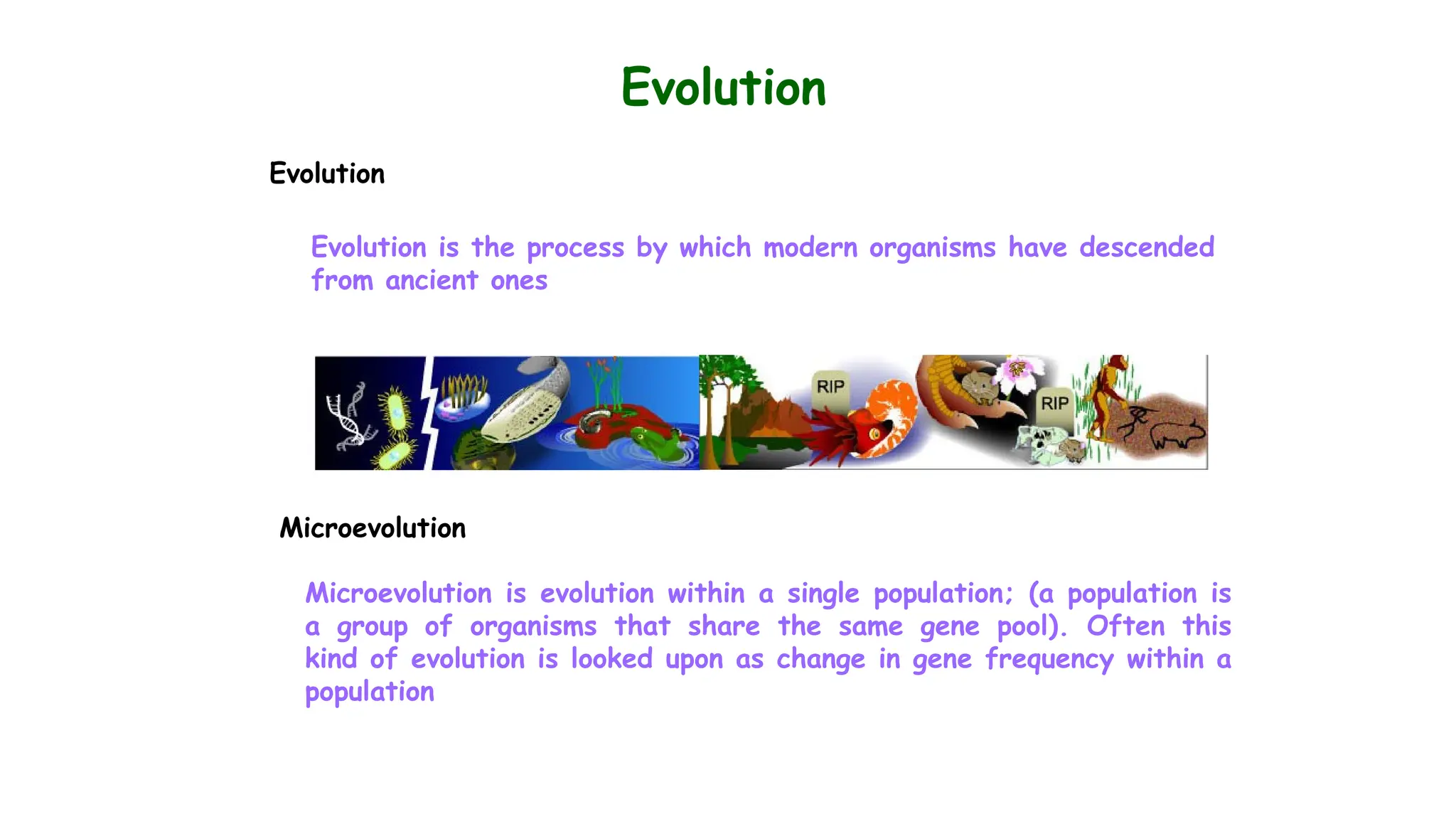
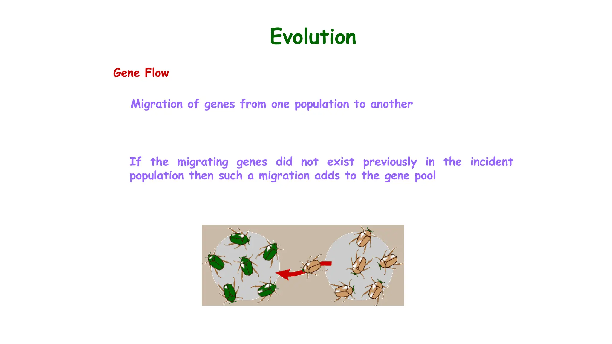
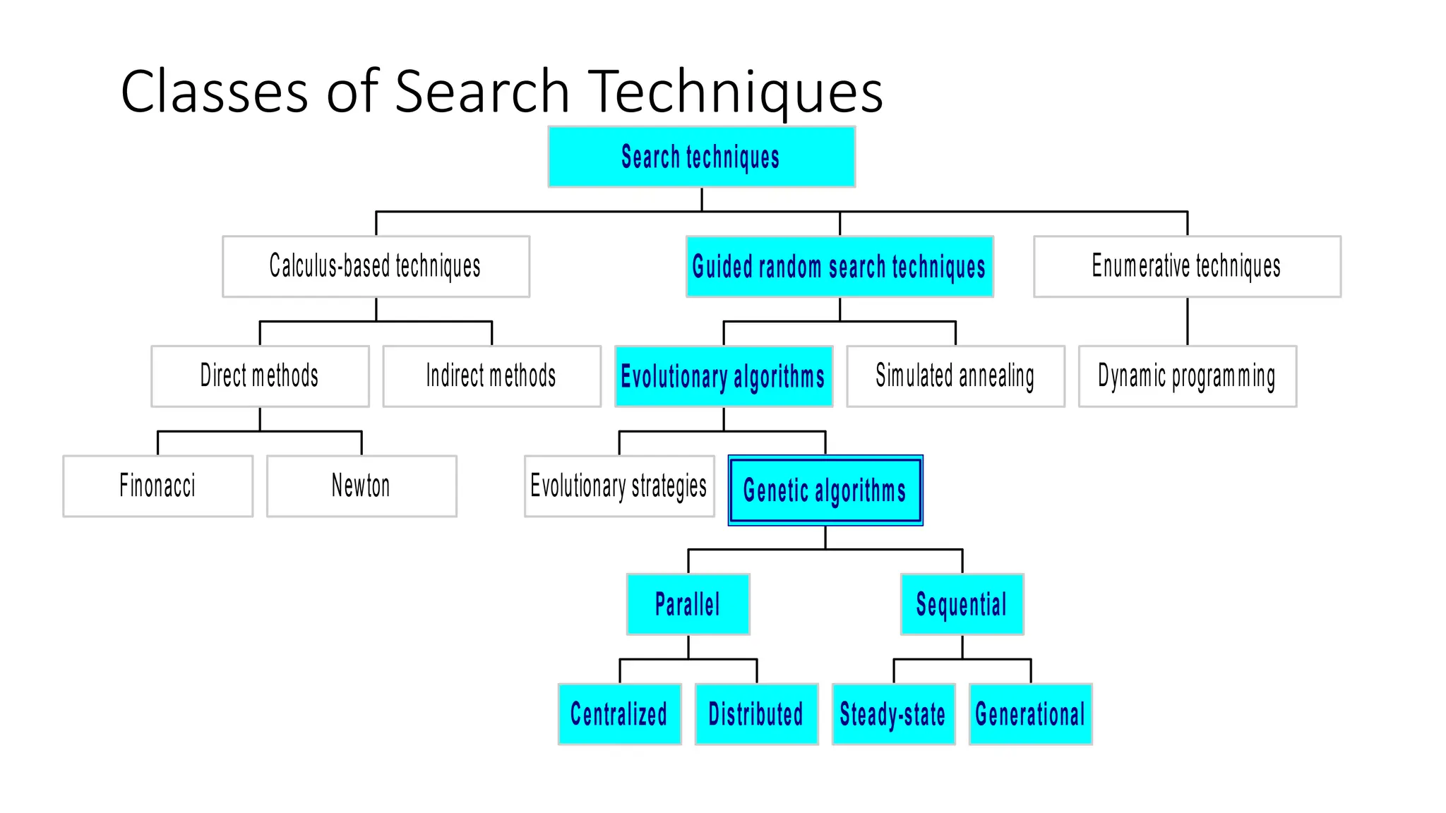
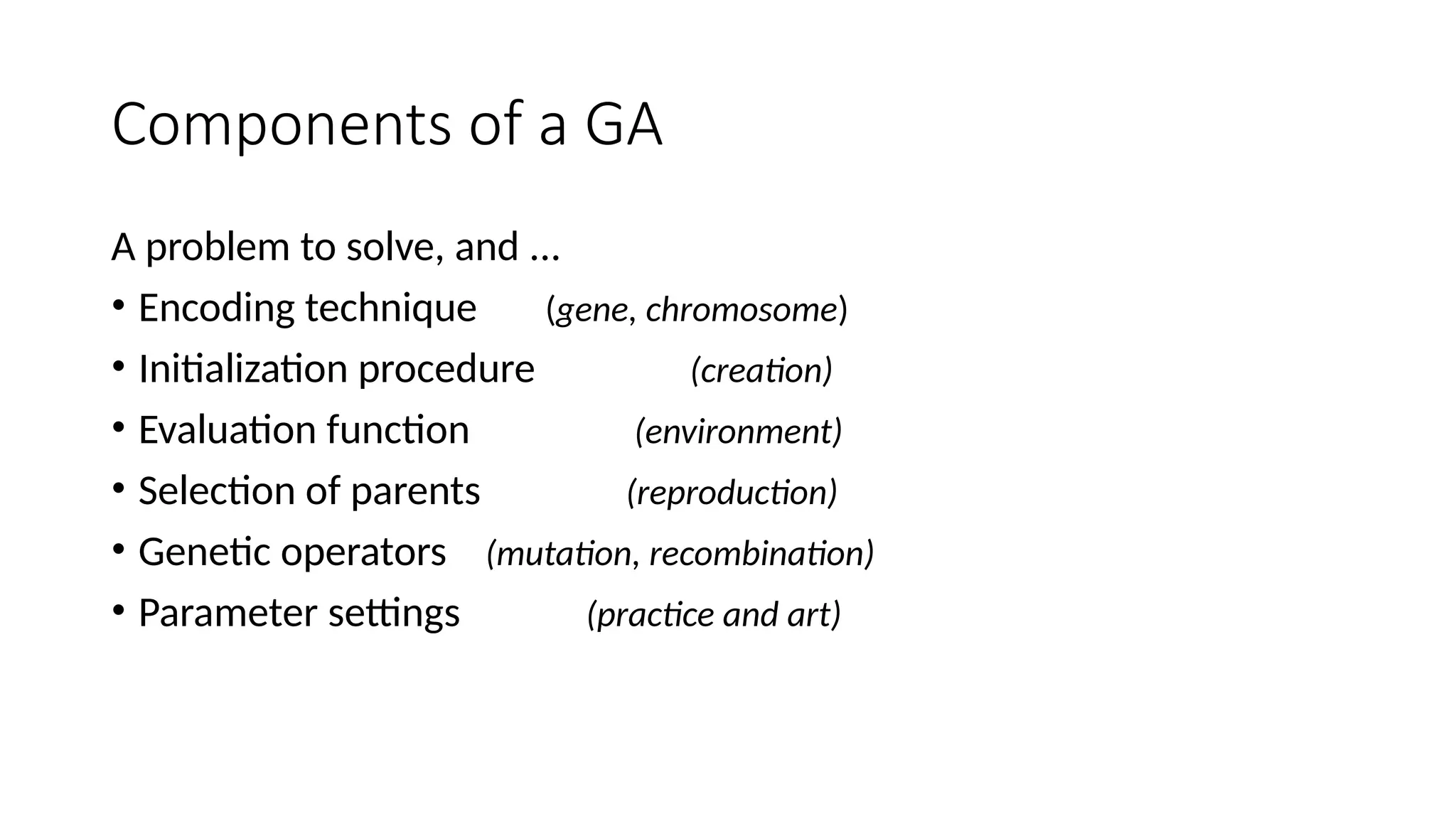
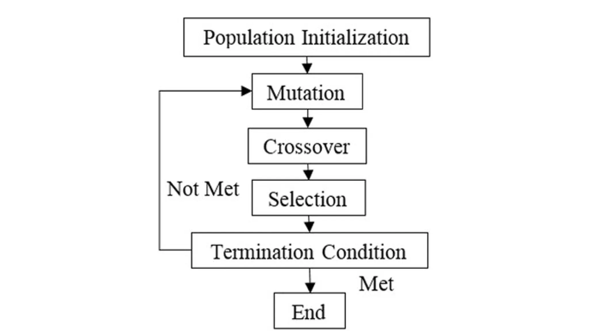
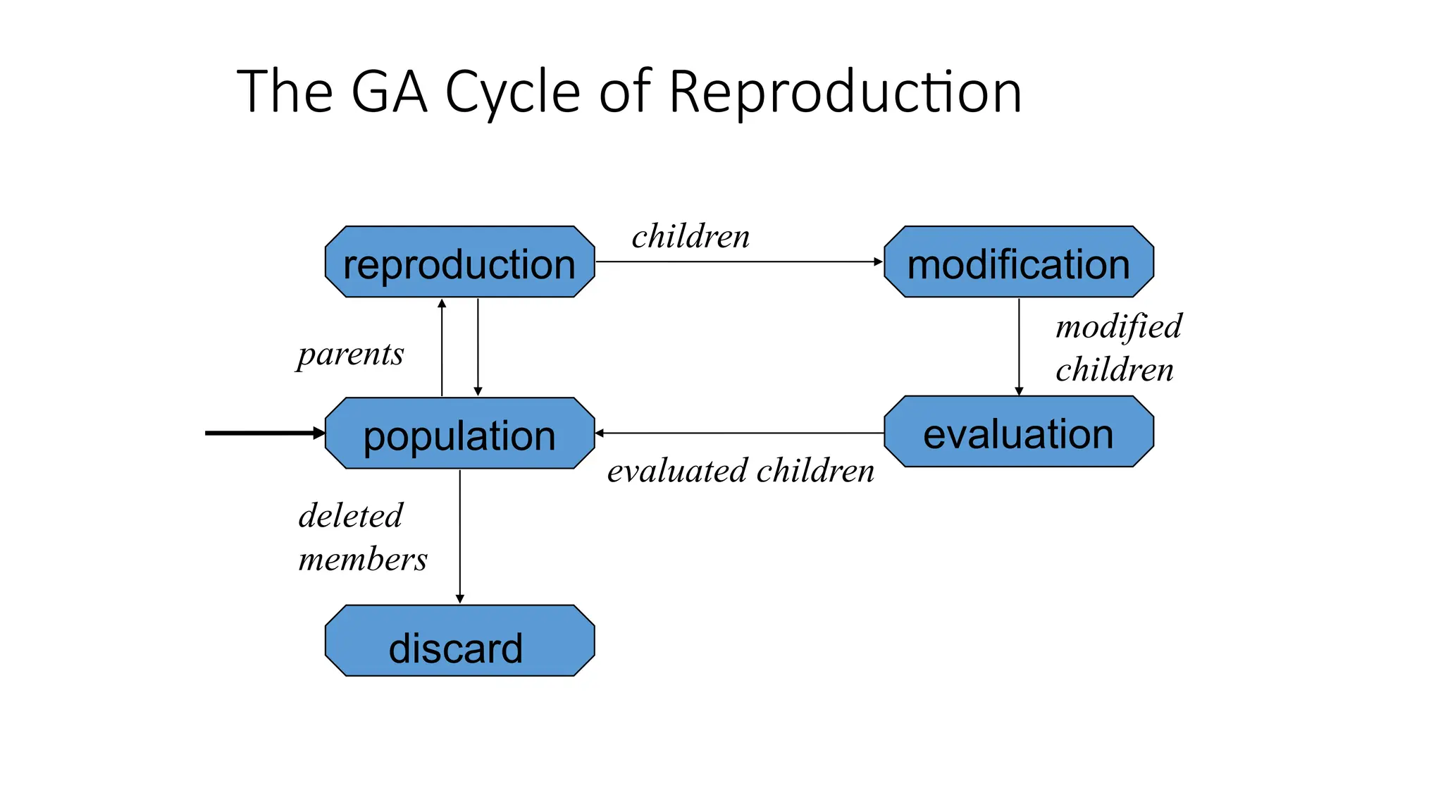
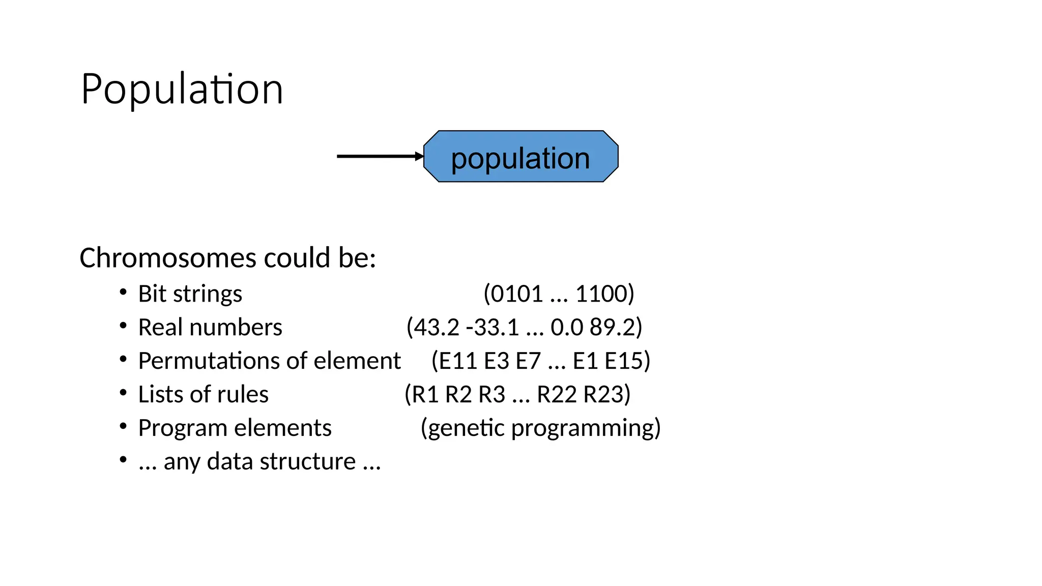
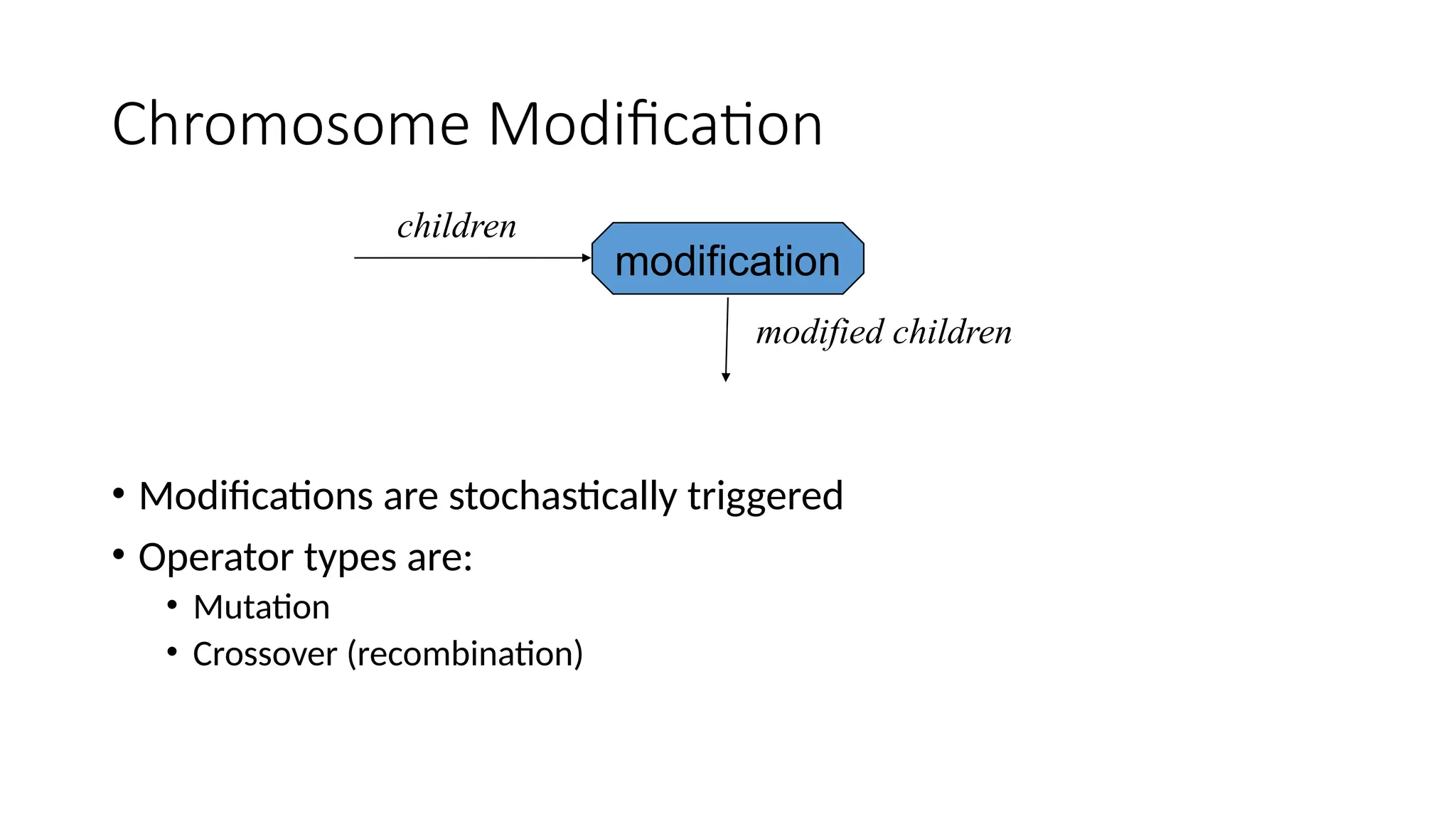
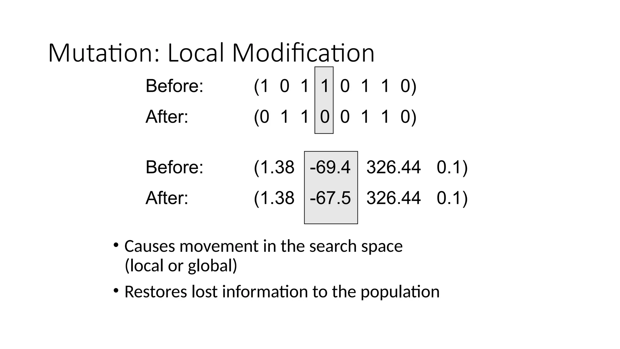
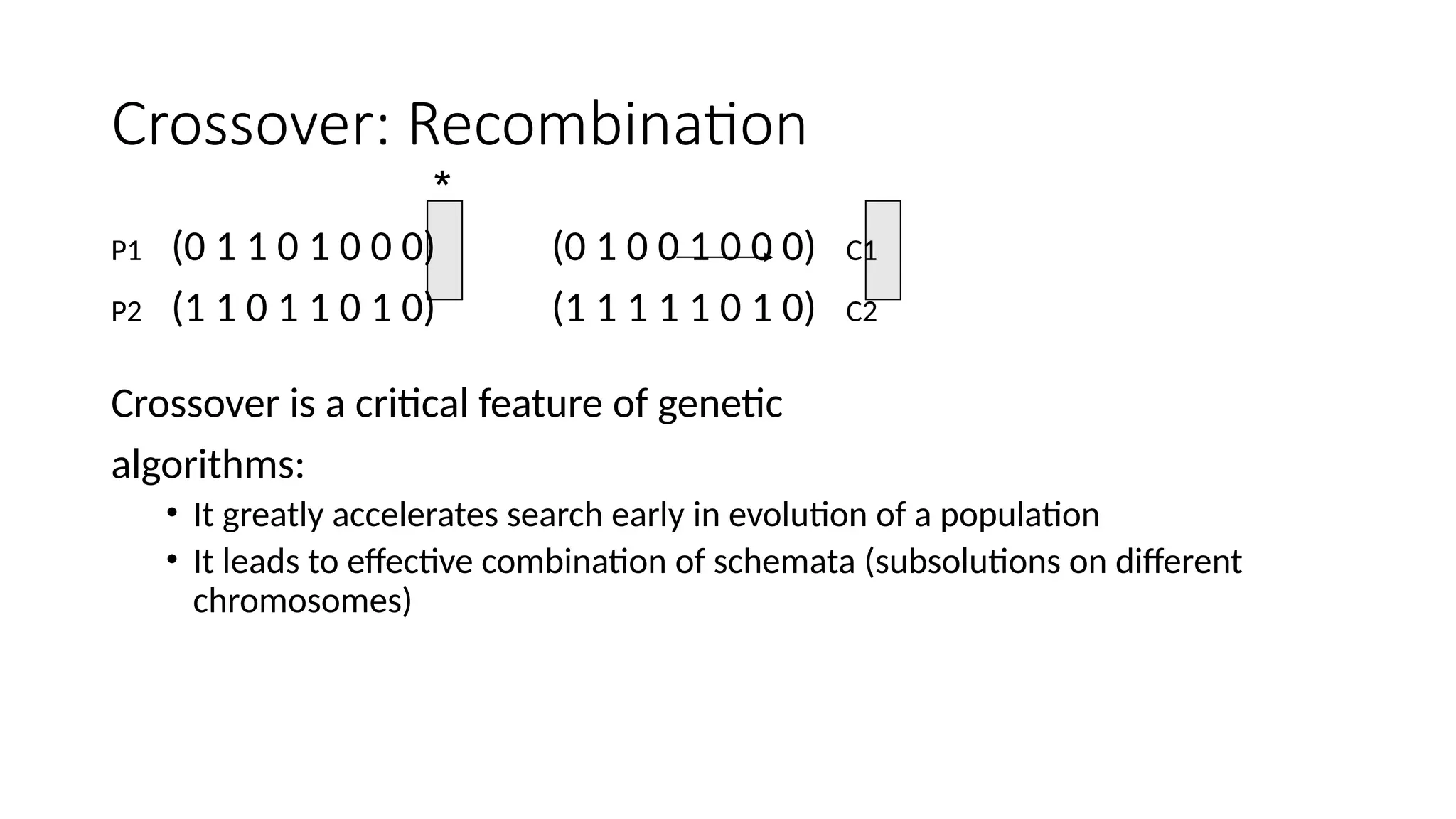
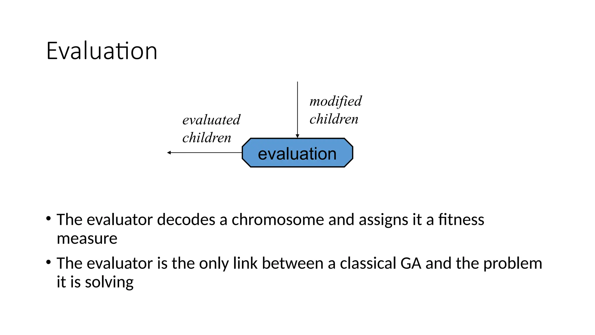
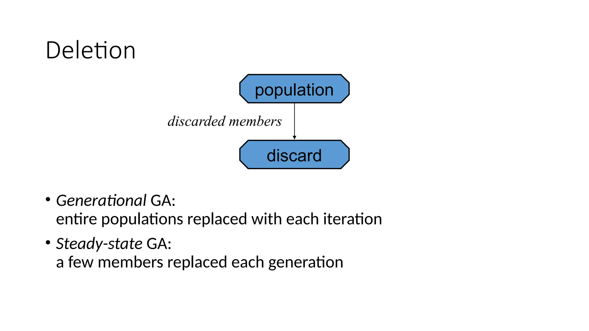
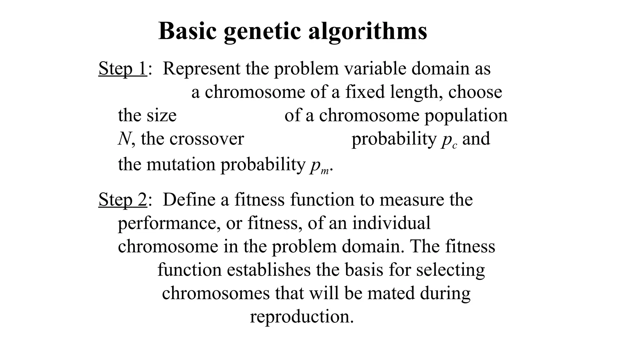
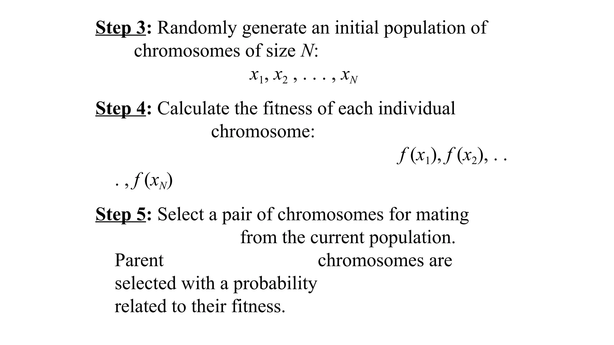
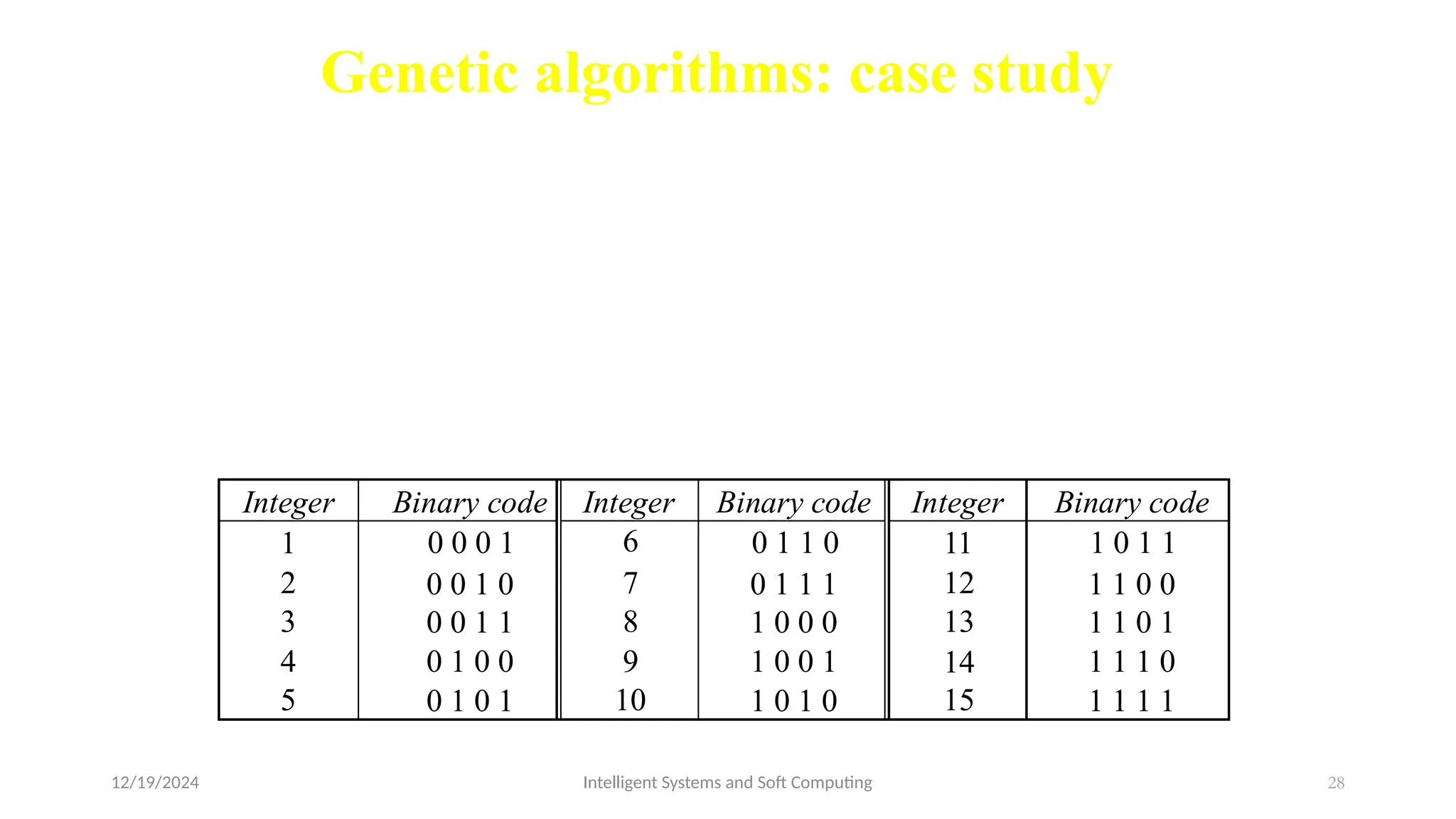
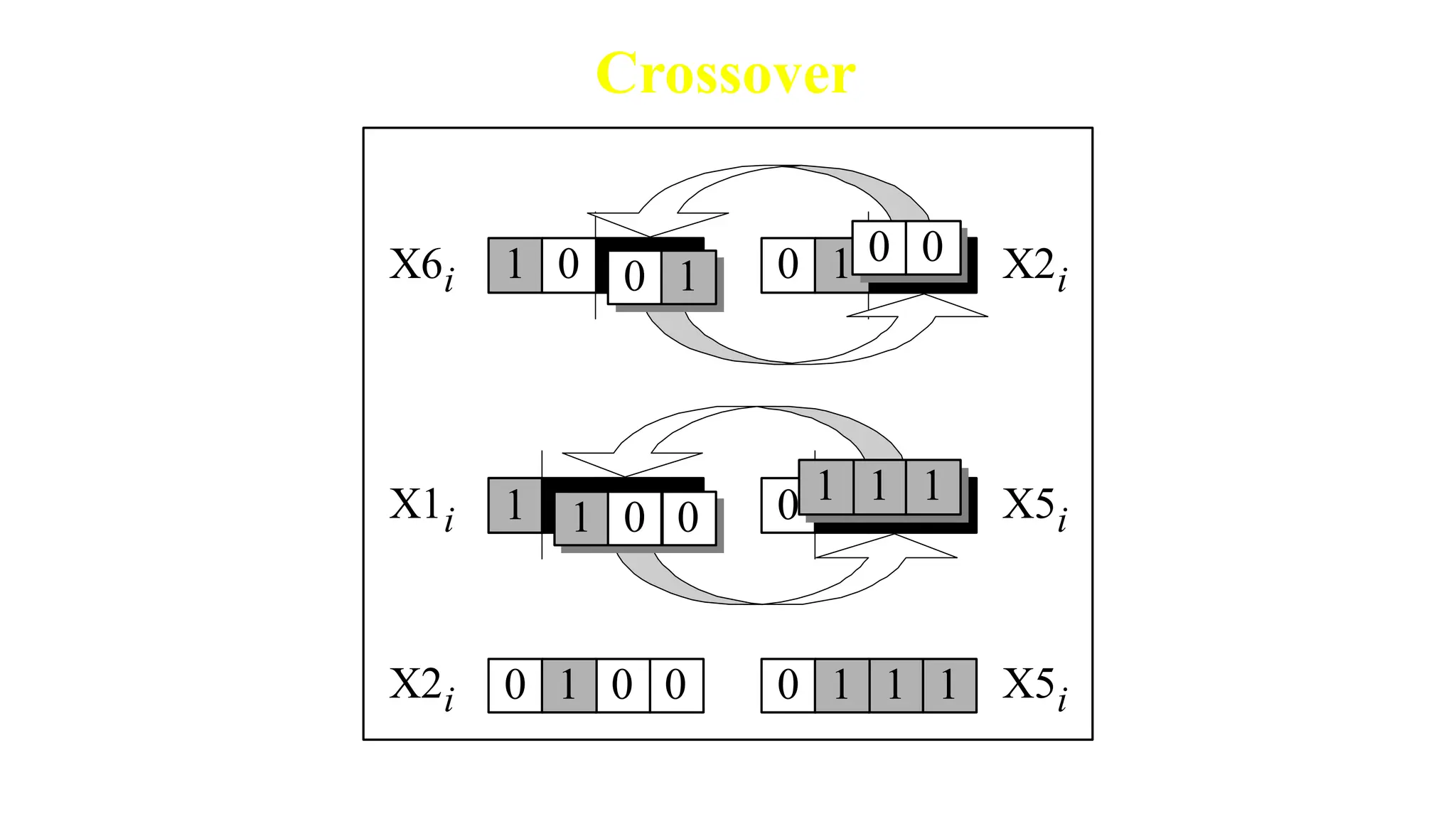
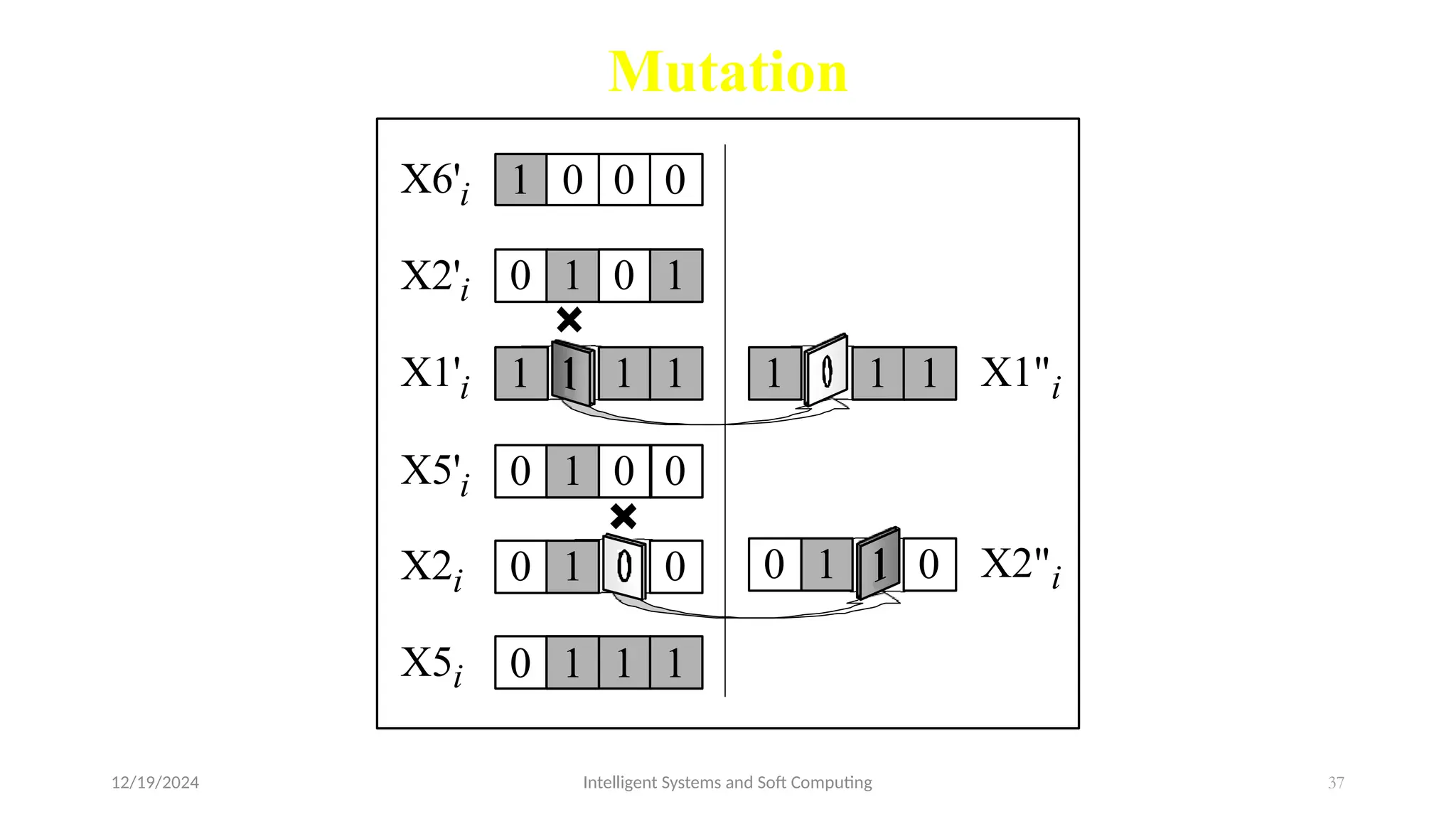
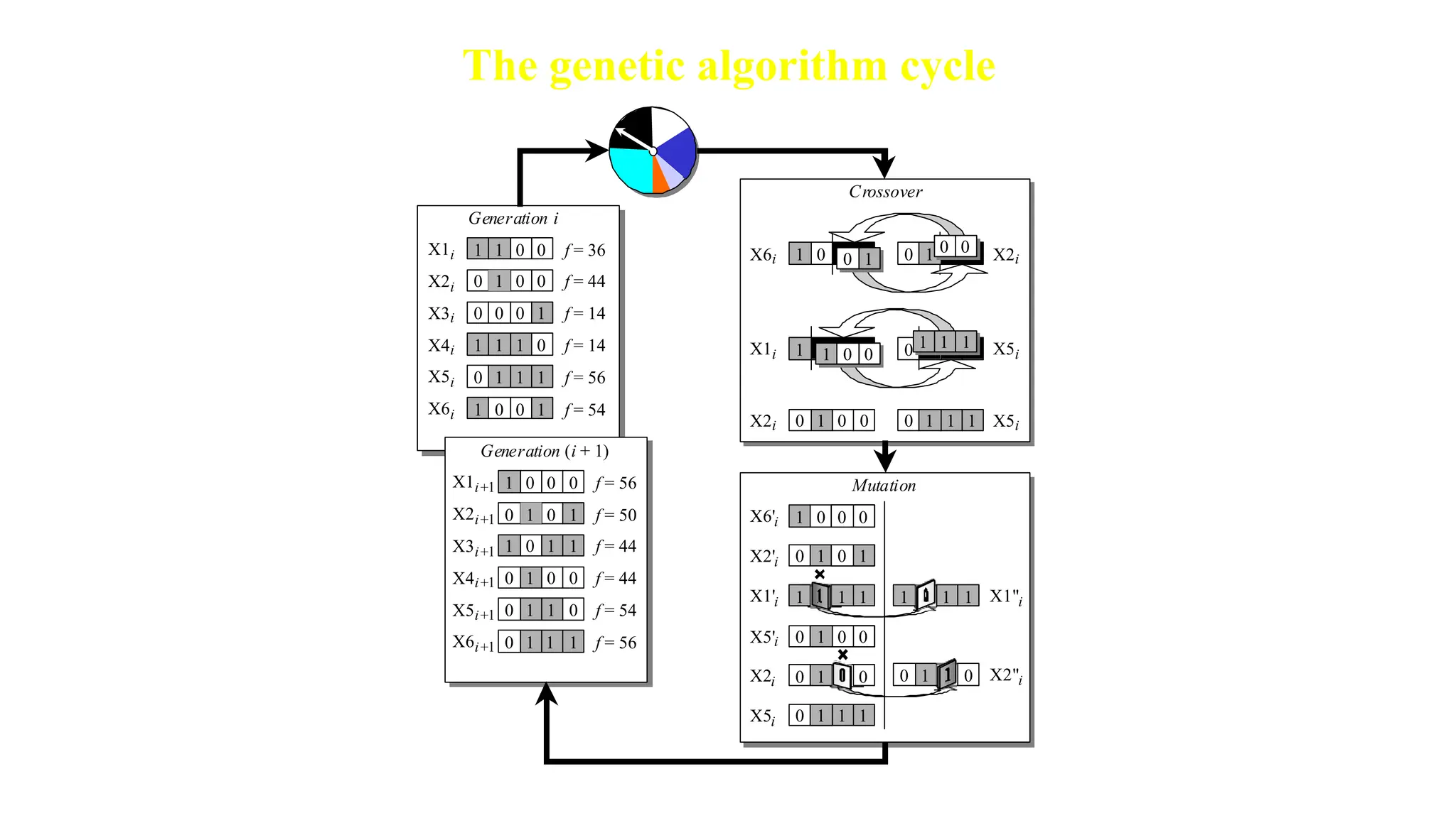
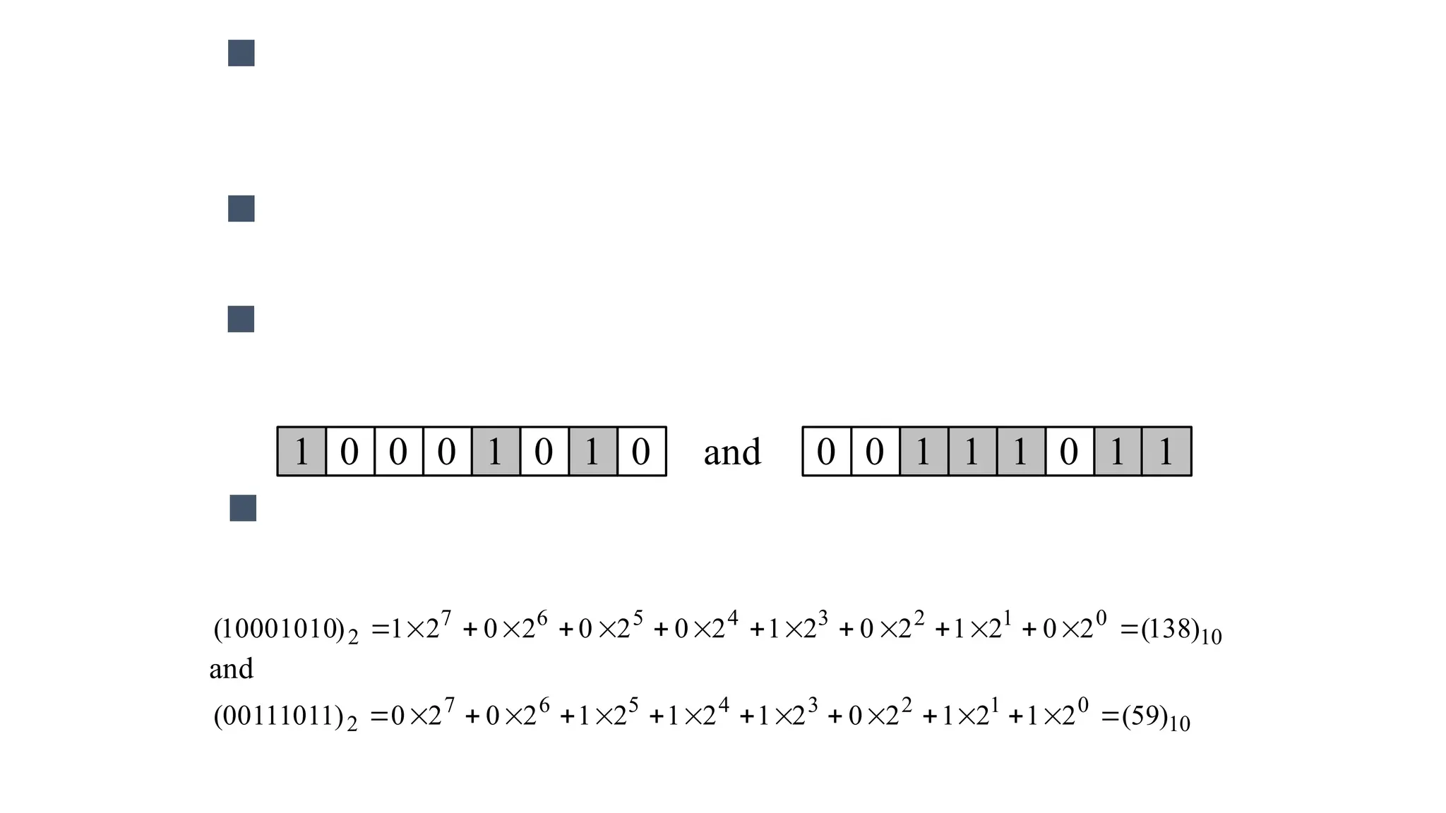
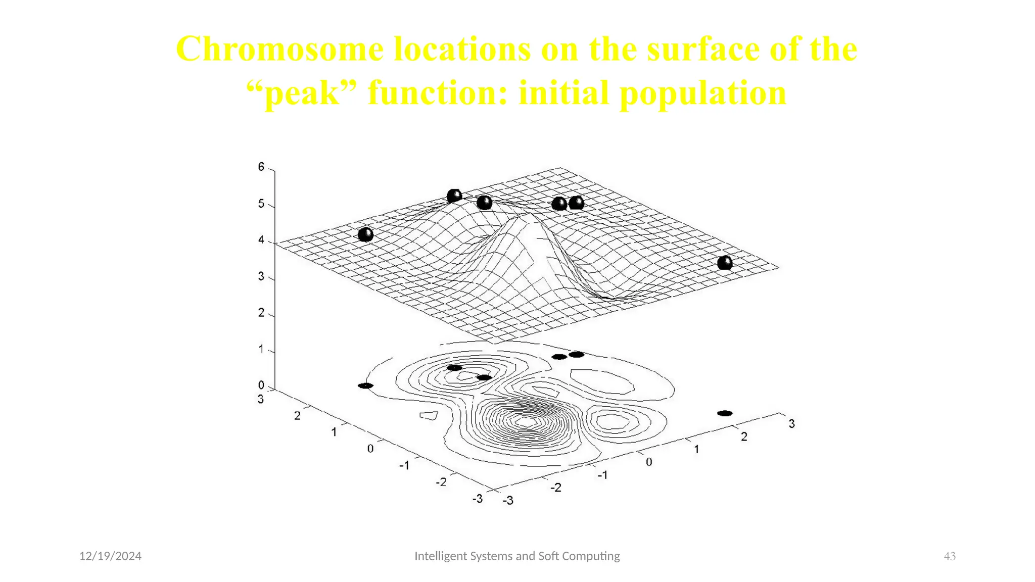
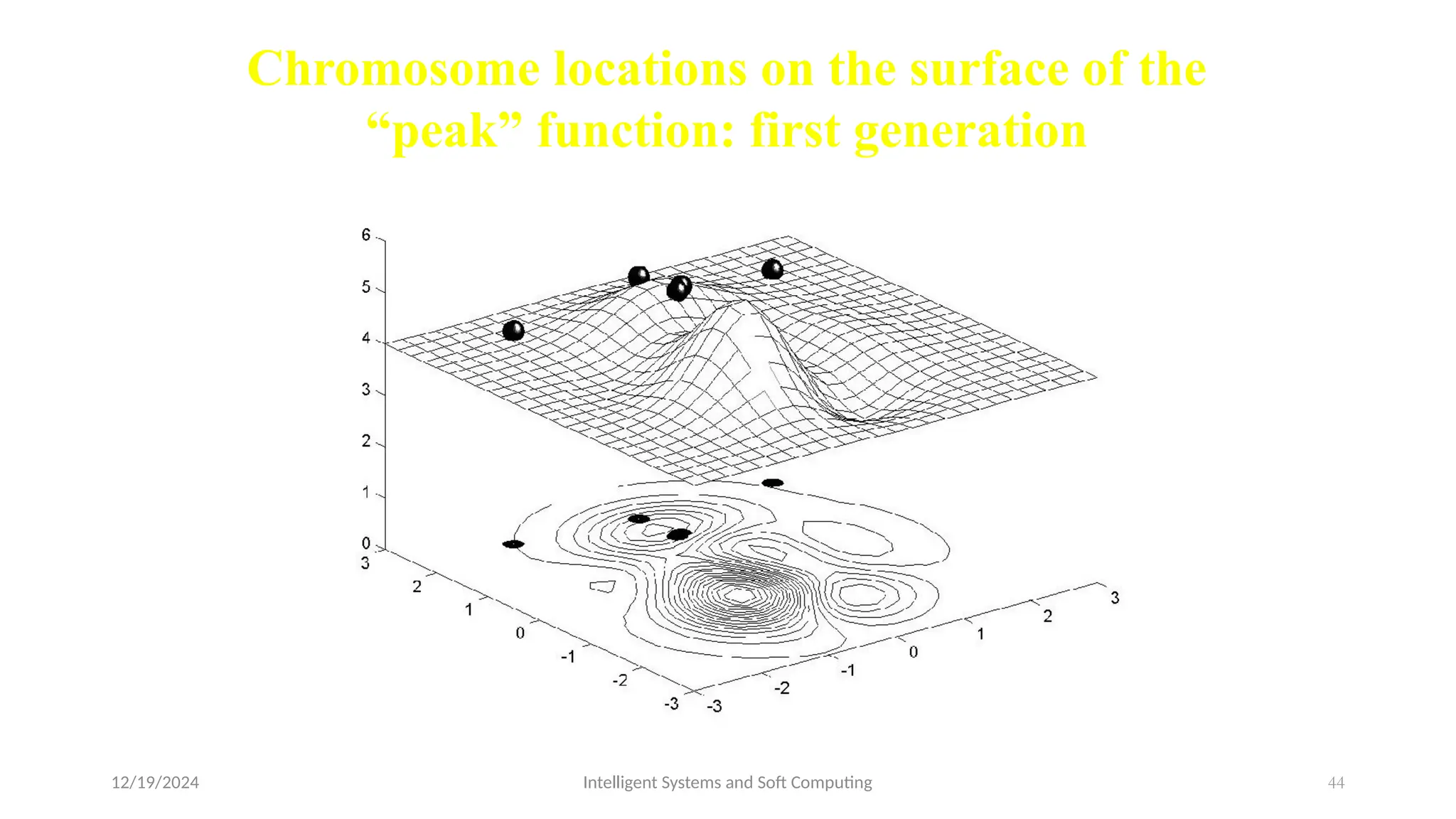
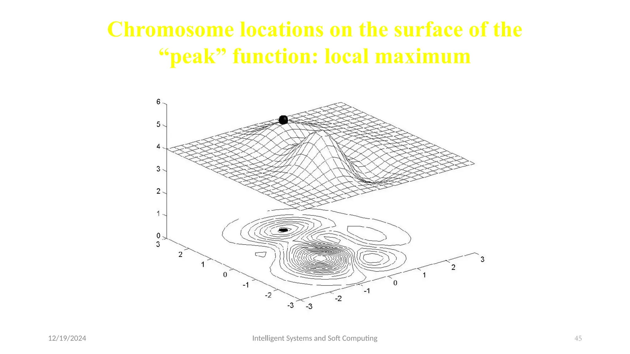
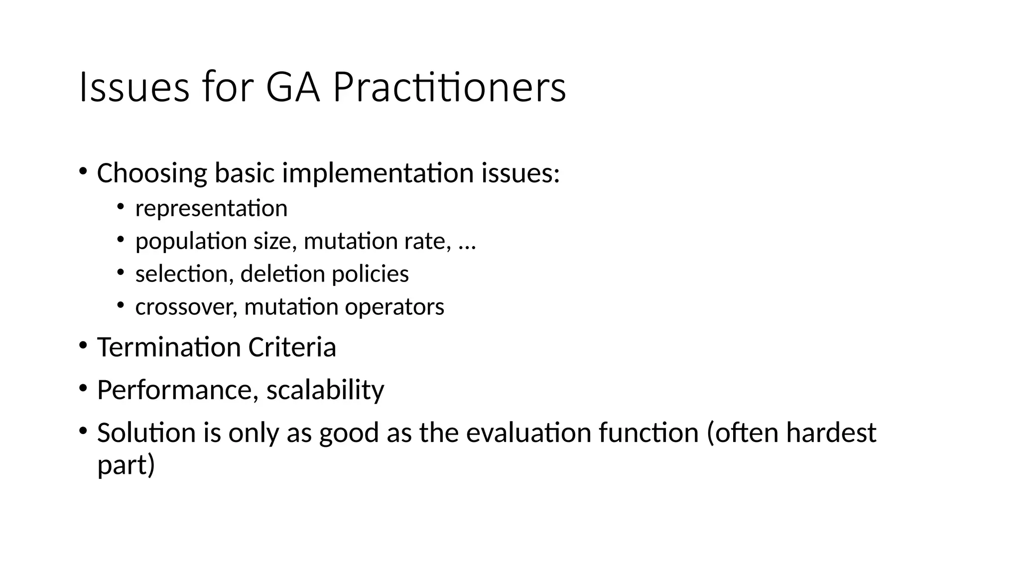
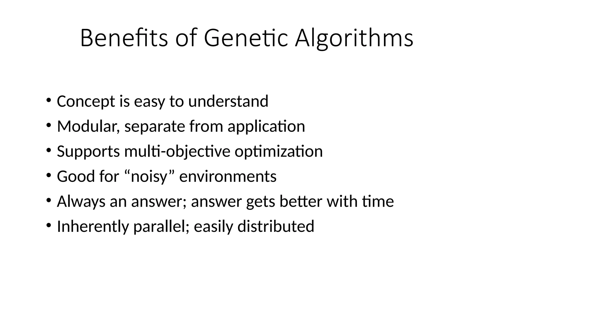
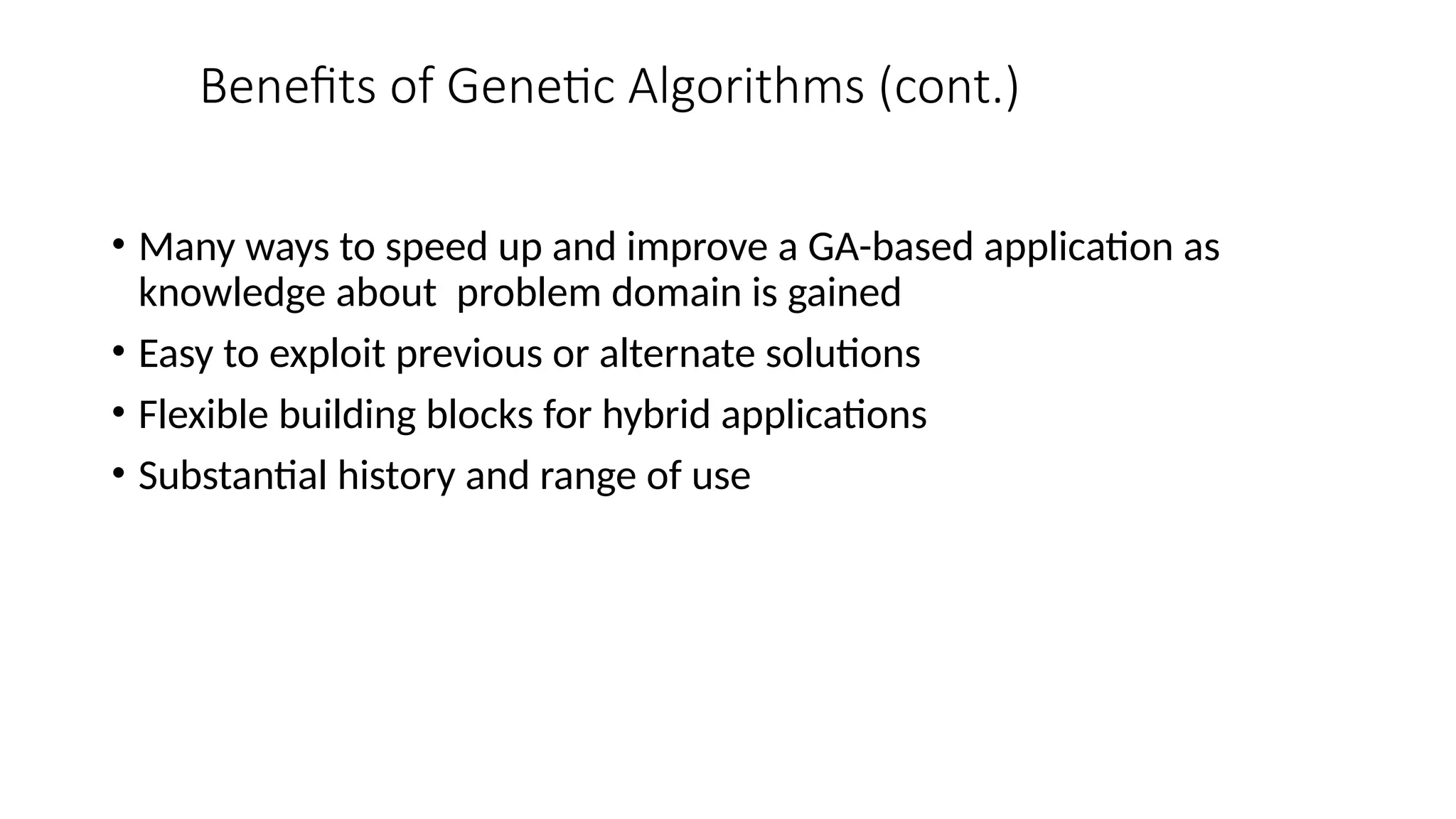
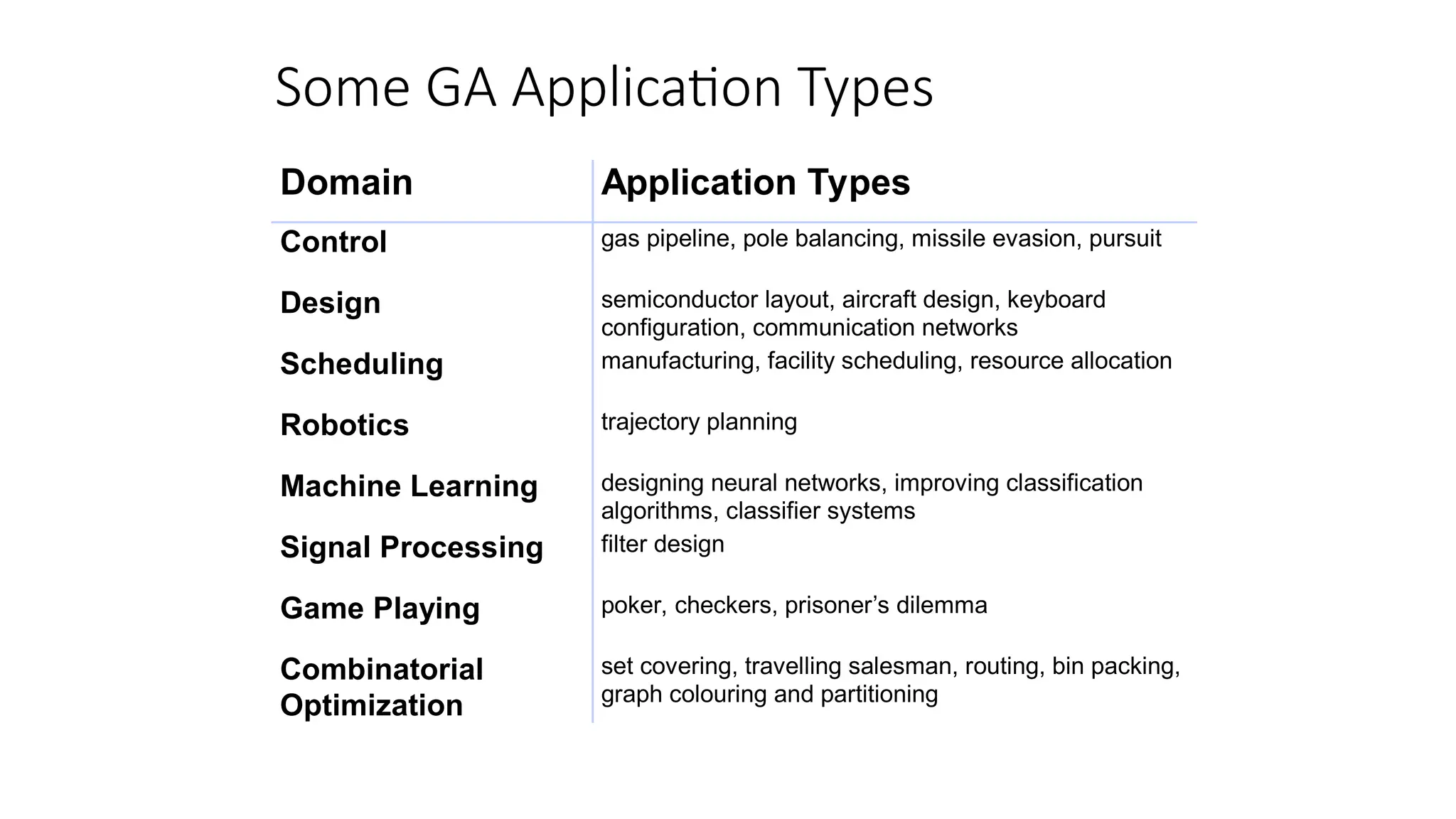
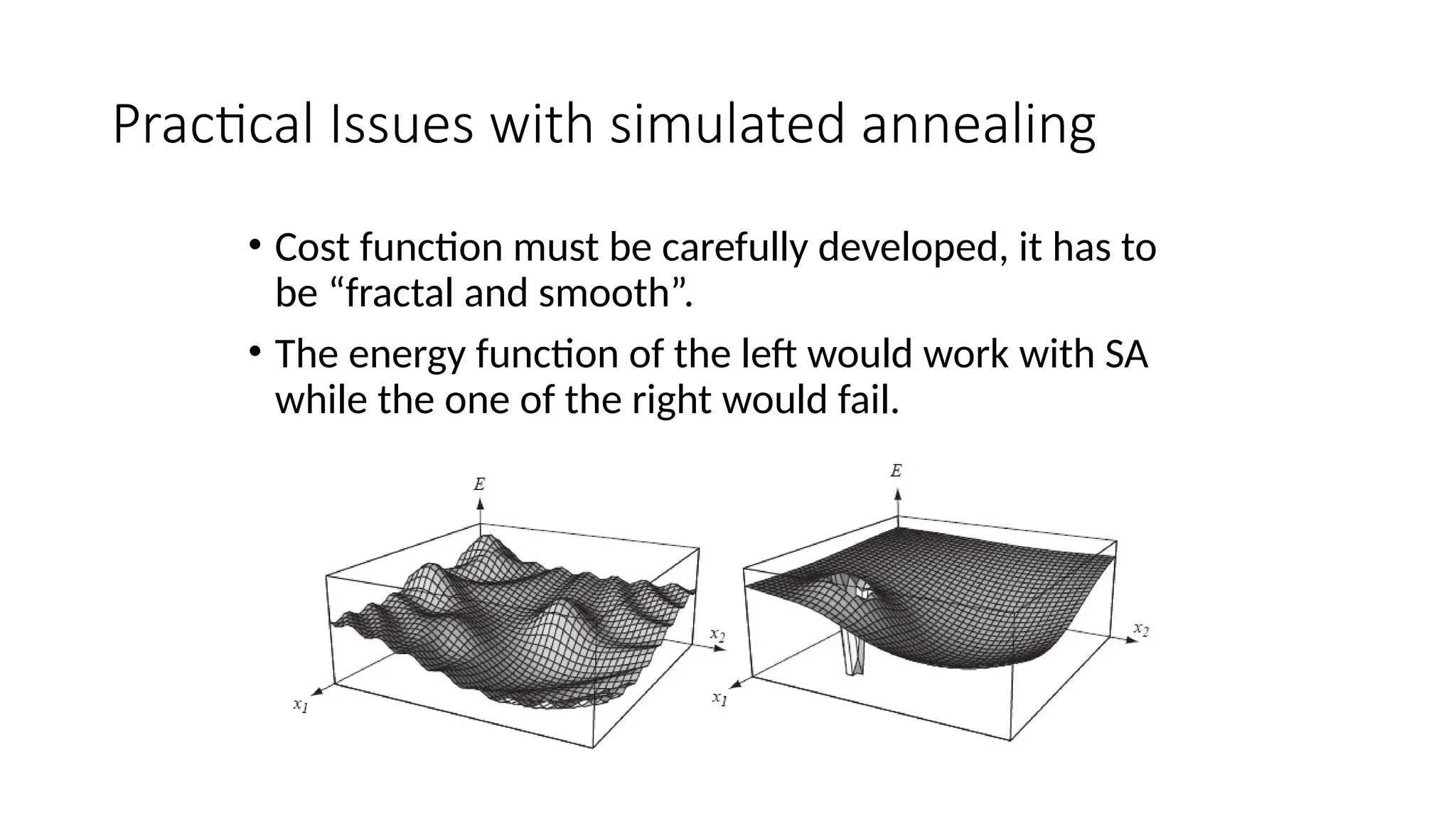
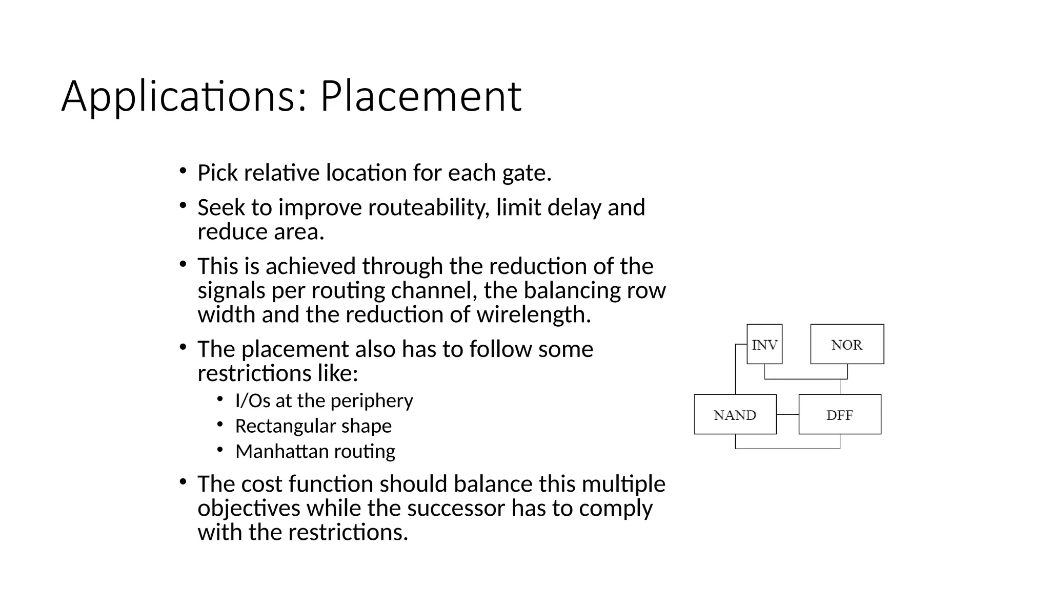
KEMBAR78
Genetic algorithm optimization technique.pptx
Optimization
V Velmurugan
Associate Professor
School of Electronics Engineering
Email: vvelmurugan@vit.ac.in
Optimization
• Introduction to evolutionary algorithms –
• Fundamentals of Genetic algorithms
• Particle Swarm Optimization
• Simulated Annealing
• Introduction to
• Neural Networks
• Neural Network based optimization
• Introduction to
• Fuzzy sets and Fuzzy Logic
• Optimization of fuzzy logic
Optimization
• noun
• the action of making the best or most effective use of a situation or resource.
• What does optimization mean in math?
• a mathematical technique for finding a maximum or minimum value of a function of several
variables subject to a set of constraints, as linear programming or systems analysis.
• What does optimizing mean in engineering?
• Lockhart and Johnson (1996) define optimization as ā€œthe process of finding the most
effective or favorable value or conditionā€. The purpose of optimization is to achieve the
ā€œbestā€ design relative to a set of prioritized criteria or constraints. This decision-making
process is known as optimization.
The Next one -Hour
Evolution
Genetic Algorithm
Some Applications of Genetic Algorithm
Particle Swarm Optimization
Simulated Annealing
•
Evolution
Evolution
Evolution is the process by which modern organisms have descended
from ancient ones
Microevolution
Microevolution is evolution within a single population; (a population is
a group of organisms that share the same gene pool). Often this
kind of evolution is looked upon as change in gene frequency within a
population
Evolution
For evolution to occur
Heredity
Information needs to be passed on from one generation to
the next
Genetic Variation
There has to be differences in the characteristics of
individuals in order for change to occur
Differential Reproduction
Some individuals need to (get to) reproduce more than others
thereby increasing the frequency of their genes in the next
generation
Evolution
Heredity
Heredity is the transfer of characteristics (or traits) from parent
to offspring through genes
Evolution
Genetic Variation
Is about variety in the population and hence presence of genetic
variation improves chances of coming up with ā€œsomething newā€
The primary mechanisms of achieving genetic variation are:
Mutations Gene Flow Sexual Reproduction
Evolution
Mutation
It is a random change in DNA
It can be beneficial, neutral or harmful to the organism
Not all mutations matter to evolution
Evolution
Gene Flow
Migration of genes from one population to another
If the migrating genes did not exist previously in the incident
population then such a migration adds to the gene pool
Evolution
Sexual Reproduction
This type of producing young can introduce new gene
combinations through genetic shuffling
The Genetic Algorithm
• Directed search algorithms based on the mechanics of biological
evolution
• Developed by John Holland, University of Michigan (1970’s)
• To understand the adaptive processes of natural systems
• To design artificial systems software that retains the robustness of natural
systems.
• Provide efficient, effective techniques for optimization and machine
learning applications
• Widely-used today in business, scientific and engineering circles
Classes of Search Techniques
Finonacci Newton
Direct methods Indirect methods
Calculus-based techniques
Evolutionary strategies
Centralized Distributed
Parallel
Steady-state Generational
Sequential
Genetic algorithms
Evolutionary algorithms Simulated annealing
Guided random search techniques
Dynamic programming
Enumerative techniques
Search techniques
Components of a GA
A problem to solve, and ...
• Encoding technique (gene, chromosome)
• Initialization procedure (creation)
• Evaluation function (environment)
• Selection of parents (reproduction)
• Genetic operators (mutation, recombination)
• Parameter settings (practice and art)
Simple Genetic Algorithm
{
initialize population;
evaluate population;
while TerminationCriteriaNotSatisfied
{
select parents for reproduction;
perform recombination and mutation;
evaluate population;
}
}
The GA Cycle of Reproduction
reproduction
population evaluation
modification
discard
deleted
members
parents
children
modified
children
evaluated children
Population
Chromosomes could be:
• Bit strings (0101 ... 1100)
• Real numbers (43.2 -33.1 ... 0.0 89.2)
• Permutations of element (E11 E3 E7 ... E1 E15)
• Lists of rules (R1 R2 R3 ... R22 R23)
• Program elements (genetic programming)
• ... any data structure ...
population
Reproduction
reproduction
population
parents
children
Parents are selected at random with
selection chances biased in relation to
chromosome evaluations.
Chromosome Modification
modification
children
• Modifications are stochastically triggered
• Operator types are:
• Mutation
• Crossover (recombination)
modified children
Mutation: Local Modification
Before: (1 0 1 1 0 1 1 0)
After: (0 1 1 0 0 1 1 0)
Before: (1.38 -69.4 326.44 0.1)
After: (1.38 -67.5 326.44 0.1)
• Causes movement in the search space
(local or global)
• Restores lost information to the population
Crossover: Recombination
P1 (0 1 1 0 1 0 0 0) (0 1 0 0 1 0 0 0) C1
P2 (1 1 0 1 1 0 1 0) (1 1 1 1 1 0 1 0) C2
Crossover is a critical feature of genetic
algorithms:
• It greatly accelerates search early in evolution of a population
• It leads to effective combination of schemata (subsolutions on different
chromosomes)
*
Evaluation
• The evaluator decodes a chromosome and assigns it a fitness
measure
• The evaluator is the only link between a classical GA and the problem
it is solving
evaluation
evaluated
children
modified
children
Deletion
• Generational GA:
entire populations replaced with each iteration
• Steady-state GA:
a few members replaced each generation
population
discard
discarded members
Basic genetic algorithms
Step 1: Represent the problem variable domain as
a chromosome of a fixed length, choose
the size of a chromosome population
N, the crossover probability pc and
the mutation probability pm.
Step 2: Define a fitness function to measure the
performance, or fitness, of an individual
chromosome in the problem domain. The fitness
function establishes the basis for selecting
chromosomes that will be mated during
reproduction.
Step 3: Randomly generate an initial population of
chromosomes of size N:
x1, x2 , . . . , xN
Step 4: Calculate the fitness of each individual
chromosome:
f (x1), f (x2), . .
. , f (xN)
Step 5: Select a pair of chromosomes for mating
from the current population.
Parent chromosomes are
selected with a probability
related to their fitness.
Step 6: Create a pair of offspring chromosomes by
applying the genetic operators - crossover and
mutation.
Step 7: Place the created offspring chromosomes
in the new population.
Step 8: Repeat Step 5 until the size of the new
chromosome population becomes equal to the
size of the initial population,
N.
Step 9: Replace the initial (parent) chromosome
population with the new (offspring)
population.
Step 10: Go to Step 4, and repeat the process until
the termination criterion is satisfied.
12/19/2024 Intelligent Systems and Soft Computing 28
Genetic algorithms: case study
A simple example will help us to understand how
a GA works. Let us find the maximum value of
the function (15x - x2) where parameter x varies
between 0 and 15. For simplicity, we may
assume that x takes only integer values. Thus,
chromosomes can be built with only four genes:
Integer Binary code Integer Binary code Integer Binary code
1 11
2 7 12
3 8 13
4 9 14
5 10 15
6 1 0 1 1
1 1 0 0
1 1 0 1
1 1 1 0
1 1 1 1
0 1 1 0
0 1 1 1
1 0 0 0
1 0 0 1
1 0 1 0
0 0 0 1
0 0 1 0
0 0 1 1
0 1 0 0
0 1 0 1
12/19/2024 Intelligent Systems and Soft Computing 29
Suppose that the size of the chromosome population
N is 6, the crossover probability pc equals
0.7, and the mutation probability pm
equals 0.001. The fitness function in
our example is defined by
f(x) = 15 x – x2
12/19/2024 Intelligent Systems and Soft Computing 30
The fitness function and chromosome locations
Chromosome
label
Chromosome
string
Decoded
integer
Chromosome
fitness
Fitness
ratio, %
X1 1 1 0 0 12 36 16.5
X2 0 1 0 0 4 44 20.2
X3 0 0 0 1 1 14 6.4
X4 1 1 1 0 14 14 6.4
X5 0 1 1 1 7 56 25.7
X6 1 0 0 1 9 54 24.8
x
50
40
30
20
60
10
0
0 5 10 15
f(x)
(a) Chromosome initial locations.
x
50
40
30
20
60
10
0
0 5 10 15
(b) Chromosome final locations.
12/19/2024 Intelligent Systems and Soft Computing 31
 In natural selection, only the fittest species can
survive, breed, and thereby pass their genes
on to the next generation. GAs use a
similar approach, but unlike nature,
the size of the chromosome population
remains unchanged from one
generation to the next.
 The last column in Table shows the ratio of the
individual chromosome’s fitness to the
population’s total fitness. This ratio determines
the chromosome’s chance of being selected for
mating. The chromosome’s average fitness
improves from one generation to the next.
Roulette wheel selection
The most commonly used chromosome selection
techniques is the roulette wheel selection.
100 0
36.7
43.1
49.5
75.2
X1: 16.5%
X2: 20.2%
X3: 6.4%
X4: 6.4%
X5: 25.3%
X6: 24.8%
Crossover operator
 In our example, we have an initial population of 6
chromosomes. Thus, to establish the same
population in the next generation, the
roulette wheel would be
spun six times.
 Once a pair of parent chromosomes is selected,
the crossover operator is applied.
 First, the crossover operator randomly chooses a
crossover point where two parent
chromosomes ā€œbreakā€, and then
exchanges the chromosome
parts after that point. As a result, two new
offspring are created.
 If a pair of chromosomes does not cross over,
then the chromosome cloning takes place, and the
offspring are created as exact copies of each
parent.
Crossover
X6i 1 0
0 0 0
1 0 X2i
0 0
1 0
X2i 0 1
1 1 X5i
0
X1i 0 1
1 1 X5i
1 0
1 0
0 1
0 0
1
1 1
0
1 0
Mutation operator
 Mutation represents a change in the gene.
 The mutation probability is quite small in nature,
and is kept low for GAs, typically in the range
between 0.001 and 0.01.
 The mutation operator flips a randomly selected
gene in a chromosome.
 Mutation is a background operator. Its role is to
provide a guarantee that the search algorithm is
not trapped on a local optimum.
12/19/2024 Intelligent Systems and Soft Computing 37
Mutation
0 1
1 1
X5'i 0
1 0
X6'i 1 0
0
0 0
1 0
X2'i 0 1
0 0
0 1 1
1
1
X5i
1 1 1 X1"i
1 1
X2"i
0 1 0
0
X1'i 1 1 1
0 1 0
X2i
The genetic algorithm cycle
1 0
1 0
X1i
Generation i
0 0
1 0
X2i
0 0
0 1
X3i
1 1
1 0
X4i
0 1
1 1
X5i f = 56
1 0
0 1
X6i f = 54
f = 36
f = 44
f = 14
f = 14
1 0
0 0
X1i+1
Generation (i + 1)
0 0
1 1
X2i+1
1 1
0 1
X3i+1
0 0
1 0
X4i+1
0 1
1 0
X5i+1 f = 54
0 1
1 1
X6i+1 f = 56
f = 56
f = 50
f = 44
f = 44
Crossover
X6i 1 0
0 0 0
1 0 X2i
0 0
1 0
X2i 0 1
1 1 X5i
0
X1i 0 1
1 1 X5i
1 0
1 0
0 1
0 0
1
1 1
0
1 0
Mutation
0 1
1 1
X5'i 0
1 0
X6'i 1 0
0
0 0
1 0
X2'i 0 1
0 0
0 1 1
1
1
X5i
1 1 1 X1"i
1 1
X2"i
0 1 0
0
X1'i 1 1 1
0 1 0
X2i
Genetic algorithms: case study
 Suppose it is desired to find the maximum of the
ā€œpeakā€ function of two variables:
 The first step is to represent the problem variables
as a chromosome - parameters x
and y as a concatenated
binary string:
2
2
2
2
)
(
)
1
(
)
,
( 3
3
)
1
(
2 y
x
y
x
e
y
x
x
e
x
y
x
f 









1 0
0 0 1 1
0 0 0 1
0 1 1 1
0 1
y
x
where parameters x and y vary between -3 and 3.
 We also choose the size of the chromosome
population, for instance 6, and randomly
generate an initial population.
 Then these strings are converted from binary
(base 2) to decimal (base 10):
1 0
0 0 1 1
0 0 0 1
0 1 1 1
0 1
and
10
0
1
2
3
4
5
6
7
2 )
138
(
2
0
2
1
2
0
2
1
2
0
2
0
2
0
2
1
)
10001010
( 
ļ‚“

ļ‚“

ļ‚“

ļ‚“

ļ‚“

ļ‚“

ļ‚“

ļ‚“

and
10
0
1
2
3
4
5
6
7
2 )
59
(
2
1
2
1
2
0
2
1
2
1
2
1
2
0
2
0
)
00111011
( 
ļ‚“

ļ‚“

ļ‚“

ļ‚“

ļ‚“

ļ‚“

ļ‚“

ļ‚“

 First, a chromosome, that is a string of 16 bits, is
partitioned into two 8-bit strings:
 The next step is to calculate the fitness of each
chromosome. This is done in two stages.
12/19/2024 Intelligent Systems and Soft Computing 41
 Now the range of integers that can be handled by
8-bits, that is the range from 0 to (28
- 1),
is mapped to the actual range of
parameters x and y, that is the
range from -3 to 3:
 To obtain the actual values of x and y, we multiply
their decimal values by
0.0235294 and subtract 3 from
the results:
0235294
.
0
1
256
6


2470588
.
0
3
0235294
.
0
)
138
( 10 

ļ‚“

x
and
6117647
.
1
3
0235294
.
0
)
59
( 10 


ļ‚“

y
12/19/2024 Intelligent Systems and Soft Computing 42
 Using decoded values of x and y as inputs in the
mathematical function, the GA calculates
the fitness of each
chromosome.
 To find the maximum of the ā€œpeakā€ function, we
will use crossover with the probability equal to 0.7
and mutation with the probability equal to 0.001.
As we mentioned earlier, a common practice in
GAs is to specify the number of generations.
Suppose the desired number of generations is 100.
That is, the GA will create 100 generations of 6
chromosomes before stopping.
12/19/2024 Intelligent Systems and Soft Computing 43
Chromosome locations on the surface of the
ā€œpeakā€ function: initial population
12/19/2024 Intelligent Systems and Soft Computing 44
Chromosome locations on the surface of the
ā€œpeakā€ function: first generation
12/19/2024 Intelligent Systems and Soft Computing 45
Chromosome locations on the surface of the
ā€œpeakā€ function: local maximum
12/19/2024 Intelligent Systems and Soft Computing 46
Chromosome locations on the surface of the
ā€œpeakā€ function: global maximum
12/19/2024 Intelligent Systems and Soft Computing 47
Performance graphs for 100 generations of 6
chromosomes: local maximum
pc = 0.7, pm = 0.001
G e n e r a t i o n s
Best
Average
80 90 100
60 70
40 50
20 30
10
0
-0.1
0.5
0.6
0.7
0
0.1
0.2
0.3
0.4
F
i
t
n
e
s
s
12/19/2024 Intelligent Systems and Soft Computing 48
Performance graphs for 100 generations of 6
chromosomes: global maximum
Best
Average
100
G e n e r a t i o n s
80 90
60 70
40 50
20 30
10
pc = 0.7, pm = 0.01
1.8
0
0.2
0.4
0.6
0.8
1.0
1.2
1.4
1.6
F
i
t
n
e
s
s
12/19/2024 Intelligent Systems and Soft Computing 49
Performance graphs for 20 generations of
60 chromosomes
pc = 0.7, pm = 0.001
Best
Average
20
G e n e r a t i o n s
16 18
12 14
8 10
46
2
0
0.2
0.4
0.6
0.8
1.0
1.2
1.4
1.6
1.8
F
i
t
n
e
s
s
Genetic Algorithms (IX)
Issues
Generation of initial population
Evaluation
Reproduction operation
Crossover and Mutation operations and
feasibility issues
Representation
Genetic Algorithms
Benefits to engineers as an optimization tool
Problem formulation is easier
Allows external procedure based declarations
Can work naturally in a discrete environment
Issues for GA Practitioners
• Choosing basic implementation issues:
• representation
• population size, mutation rate, ...
• selection, deletion policies
• crossover, mutation operators
• Termination Criteria
• Performance, scalability
• Solution is only as good as the evaluation function (often hardest
part)
Benefits of Genetic Algorithms
• Concept is easy to understand
• Modular, separate from application
• Supports multi-objective optimization
• Good for ā€œnoisyā€ environments
• Always an answer; answer gets better with time
• Inherently parallel; easily distributed
Benefits of Genetic Algorithms (cont.)
• Many ways to speed up and improve a GA-based application as
knowledge about problem domain is gained
• Easy to exploit previous or alternate solutions
• Flexible building blocks for hybrid applications
• Substantial history and range of use
When to Use a GA
• Alternate solutions are too slow or overly complicated
• Need an exploratory tool to examine new approaches
• Problem is similar to one that has already been successfully solved by using
a GA
• Want to hybridize with an existing solution
• Benefits of the GA technology meet key problem requirements
Some GA Application Types
Domain Application Types
Control gas pipeline, pole balancing, missile evasion, pursuit
Design semiconductor layout, aircraft design, keyboard
configuration, communication networks
Scheduling manufacturing, facility scheduling, resource allocation
Robotics trajectory planning
Machine Learning designing neural networks, improving classification
algorithms, classifier systems
Signal Processing filter design
Game Playing poker, checkers, prisoner’s dilemma
Combinatorial
Optimization
set covering, travelling salesman, routing, bin packing,
graph colouring and partitioning
Simulated annealing
Local Search algorithms
• Search algorithms like breadth-first, depth-first or A* explore all the
search space systematically by keeping one or more paths in memory
and by recording which alternatives have been explored.
• When a goal is found, the path to that goal constitutes a solution.
• Local search algorithms can be very helpful if we are interested in the
solution state but not in the path to that goal. They operate only on
the current state and move into neighboring states .
Local Search algorithms
• Local search algorithms have 2 key advantages:
• They use very little memory
• They can find reasonable solutions in large or infinite (continuous) state
spaces.
• Some examples of local search algorithms are:
• Hill-climbing
• Random walk
• Simulated annealing
Annealing
• Annealing is a thermal process for obtaining low energy states of a
solid in a heat bath.
• The process contains two steps:
• Increase the temperature of the heat bath to a maximum value at which the
solid melts.
• Decrease carefully the temperature of the heat bath until the particles
arrange themselves in the ground state of the solid. Ground state is a
minimum energy state of the solid.
• The ground state of the solid is obtained only if the maximum
temperature is high enough and the cooling is done slowly.
Simulated Annealing
• The process of annealing can be simulated with the Metropolis
algorithm, which is based on Monte Carlo techniques.
• We can apply this algorithm to generate a solution to combinatorial
optimization problems assuming an analogy between them and
physical many-particle systems with the following equivalences:
• Solutions in the problem are equivalent to states in a physical system.
• The cost of a solution is equivalent to the ā€œenergyā€ of a state.
Simulated Annealing
• To apply simulated annealing with optimization purposes we require the
following:
• A successor function that returns a ā€œcloseā€ neighboring solution given the actual one. This
will work as the ā€œdisturbanceā€ for the particles of the system.
• A target function to optimize that depends on the current state of the system. This function
will work as the energy of the system.
• The search is started with a randomized state. In a polling loop we will move to
neighboring states always accepting the moves that decrease the energy while
only accepting bad moves accordingly to a probability distribution dependent on
the ā€œtemperatureā€ of the system.
Simulated Annealing
• The distribution used to
decide if we accept a bad
movement is know as
Boltzman distribution.
Decrease the temperature slowly, accepting less bad moves
at each temperature level until at very low temperatures the
algorithm becomes a greedy hill-climbing algorithm.
 This distribution is very well known is in solid physics
and plays a central role in simulated annealing. Where γ
is the current configuration of the system, E γ is the
energy related with it, and Z is a normalization constant.
Simulated Annealing: the code
1. Create random initial solution γ
2. Eold=cost(γ);
3. for(temp=tempmax; temp>=tempmin;temp=next_temp(temp) ) {
4. for(i=0;i<imax; i++ ) {
5. succesor_func(γ); //this is a randomized function
6. Enew=cost(γ);
7. delta=Enew-Eold;
8. if(delta>0)
9. if(random() >= exp(-delta/K*temp);
10. undo_func(γ); //rejected bad move
11. else
12. Eold=Enew //accepted bad move
13. else
14. Eold=Enew; //always accept good moves
}
}
Simulated Annealing
• Acceptance criterion and cooling schedule
Practical Issues with simulated annealing
• Cost function must be carefully developed, it has to
be ā€œfractal and smoothā€.
• The energy function of the left would work with SA
while the one of the right would fail.
Practical Issues with simulated annealing
• The cost function should be fast it is going to be called ā€œmillionsā€ of
times.
• The best is if we just have to calculate the deltas produced by the
modification instead of traversing through all the state.
• This is dependent on the application.
Practical Issues with simulated annealing
• In asymptotic convergence simulated annealing converges to globally
optimal solutions.
• In practice, the convergence of the algorithm depends of the cooling
schedule.
• There are some suggestion about the cooling schedule but it stills
requires a lot of testing and it usually depends on the application.
Practical Issues with simulated annealing
• Start at a temperature where 50% of bad moves are accepted.
• Each cooling step reduces the temperature by 10%
• The number of iterations at each temperature should attempt to
move between 1-10 times each ā€œelementā€ of the state.
• The final temperature should not accept bad moves; this step is
known as the quenching step.
Applications
• Basic Problems
• Traveling salesman
• Graph partitioning
• Matching problems
• Graph coloring
• Scheduling
• Engineering
• VLSI design
• Placement
• Routing
• Array logic minimization
• Layout
• Facilities layout
• Image processing
• Code design in information theory
Applications: Placement
• Pick relative location for each gate.
• Seek to improve routeability, limit delay and
reduce area.
• This is achieved through the reduction of the
signals per routing channel, the balancing row
width and the reduction of wirelength.
• The placement also has to follow some
restrictions like:
• I/Os at the periphery
• Rectangular shape
• Manhattan routing
• The cost function should balance this multiple
objectives while the successor has to comply
with the restrictions.
Applications: Placement
• In placement there are multiple complex objective.
• The cost function is difficult to balance and requires testing.
• An example of cost function that balances area efficiency vs.
performance.
• Cost=c1area+c2delay+c3power+c4crosstalk
• Where the ci weights heavily depend on the application and
requirements of the project
References
• Aarst, ā€œSimulated annealing and Boltzman machinesā€, Wiley, 1989.
• Duda Hart Stork, ā€œPattern Classificationā€, Wiley Interscience, 2001.
• Otten, ā€œThe Annealing Algorithmā€, Kluwer Academic Publishers, 1989.
• Sherwani, ā€œAlgorithms for VLSI Physical Design Automationā€, Kluwer
Academic Publishers, 1999.

Genetic algorithm optimization technique.pptx

  • 1.
    Optimization V Velmurugan Associate Professor Schoolof Electronics Engineering Email: vvelmurugan@vit.ac.in
  • 2.
    Optimization • Introduction toevolutionary algorithms – • Fundamentals of Genetic algorithms • Particle Swarm Optimization • Simulated Annealing • Introduction to • Neural Networks • Neural Network based optimization • Introduction to • Fuzzy sets and Fuzzy Logic • Optimization of fuzzy logic
  • 3.
    Optimization • noun • theaction of making the best or most effective use of a situation or resource. • What does optimization mean in math? • a mathematical technique for finding a maximum or minimum value of a function of several variables subject to a set of constraints, as linear programming or systems analysis. • What does optimizing mean in engineering? • Lockhart and Johnson (1996) define optimization as ā€œthe process of finding the most effective or favorable value or conditionā€. The purpose of optimization is to achieve the ā€œbestā€ design relative to a set of prioritized criteria or constraints. This decision-making process is known as optimization.
  • 4.
    The Next one-Hour Evolution Genetic Algorithm Some Applications of Genetic Algorithm Particle Swarm Optimization Simulated Annealing •
  • 5.
    Evolution Evolution Evolution is theprocess by which modern organisms have descended from ancient ones Microevolution Microevolution is evolution within a single population; (a population is a group of organisms that share the same gene pool). Often this kind of evolution is looked upon as change in gene frequency within a population
  • 6.
    Evolution For evolution tooccur Heredity Information needs to be passed on from one generation to the next Genetic Variation There has to be differences in the characteristics of individuals in order for change to occur Differential Reproduction Some individuals need to (get to) reproduce more than others thereby increasing the frequency of their genes in the next generation
  • 7.
    Evolution Heredity Heredity is thetransfer of characteristics (or traits) from parent to offspring through genes
  • 8.
    Evolution Genetic Variation Is aboutvariety in the population and hence presence of genetic variation improves chances of coming up with ā€œsomething newā€ The primary mechanisms of achieving genetic variation are: Mutations Gene Flow Sexual Reproduction
  • 9.
    Evolution Mutation It is arandom change in DNA It can be beneficial, neutral or harmful to the organism Not all mutations matter to evolution
  • 10.
    Evolution Gene Flow Migration ofgenes from one population to another If the migrating genes did not exist previously in the incident population then such a migration adds to the gene pool
  • 11.
    Evolution Sexual Reproduction This typeof producing young can introduce new gene combinations through genetic shuffling
  • 12.
    The Genetic Algorithm •Directed search algorithms based on the mechanics of biological evolution • Developed by John Holland, University of Michigan (1970’s) • To understand the adaptive processes of natural systems • To design artificial systems software that retains the robustness of natural systems. • Provide efficient, effective techniques for optimization and machine learning applications • Widely-used today in business, scientific and engineering circles
  • 13.
    Classes of SearchTechniques Finonacci Newton Direct methods Indirect methods Calculus-based techniques Evolutionary strategies Centralized Distributed Parallel Steady-state Generational Sequential Genetic algorithms Evolutionary algorithms Simulated annealing Guided random search techniques Dynamic programming Enumerative techniques Search techniques
  • 14.
    Components of aGA A problem to solve, and ... • Encoding technique (gene, chromosome) • Initialization procedure (creation) • Evaluation function (environment) • Selection of parents (reproduction) • Genetic operators (mutation, recombination) • Parameter settings (practice and art)
  • 15.
    Simple Genetic Algorithm { initializepopulation; evaluate population; while TerminationCriteriaNotSatisfied { select parents for reproduction; perform recombination and mutation; evaluate population; } }
  • 17.
    The GA Cycleof Reproduction reproduction population evaluation modification discard deleted members parents children modified children evaluated children
  • 18.
    Population Chromosomes could be: •Bit strings (0101 ... 1100) • Real numbers (43.2 -33.1 ... 0.0 89.2) • Permutations of element (E11 E3 E7 ... E1 E15) • Lists of rules (R1 R2 R3 ... R22 R23) • Program elements (genetic programming) • ... any data structure ... population
  • 19.
    Reproduction reproduction population parents children Parents are selectedat random with selection chances biased in relation to chromosome evaluations.
  • 20.
    Chromosome Modification modification children • Modificationsare stochastically triggered • Operator types are: • Mutation • Crossover (recombination) modified children
  • 21.
    Mutation: Local Modification Before:(1 0 1 1 0 1 1 0) After: (0 1 1 0 0 1 1 0) Before: (1.38 -69.4 326.44 0.1) After: (1.38 -67.5 326.44 0.1) • Causes movement in the search space (local or global) • Restores lost information to the population
  • 22.
    Crossover: Recombination P1 (01 1 0 1 0 0 0) (0 1 0 0 1 0 0 0) C1 P2 (1 1 0 1 1 0 1 0) (1 1 1 1 1 0 1 0) C2 Crossover is a critical feature of genetic algorithms: • It greatly accelerates search early in evolution of a population • It leads to effective combination of schemata (subsolutions on different chromosomes) *
  • 23.
    Evaluation • The evaluatordecodes a chromosome and assigns it a fitness measure • The evaluator is the only link between a classical GA and the problem it is solving evaluation evaluated children modified children
  • 24.
    Deletion • Generational GA: entirepopulations replaced with each iteration • Steady-state GA: a few members replaced each generation population discard discarded members
  • 25.
    Basic genetic algorithms Step1: Represent the problem variable domain as a chromosome of a fixed length, choose the size of a chromosome population N, the crossover probability pc and the mutation probability pm. Step 2: Define a fitness function to measure the performance, or fitness, of an individual chromosome in the problem domain. The fitness function establishes the basis for selecting chromosomes that will be mated during reproduction.
  • 26.
    Step 3: Randomlygenerate an initial population of chromosomes of size N: x1, x2 , . . . , xN Step 4: Calculate the fitness of each individual chromosome: f (x1), f (x2), . . . , f (xN) Step 5: Select a pair of chromosomes for mating from the current population. Parent chromosomes are selected with a probability related to their fitness.
  • 27.
    Step 6: Createa pair of offspring chromosomes by applying the genetic operators - crossover and mutation. Step 7: Place the created offspring chromosomes in the new population. Step 8: Repeat Step 5 until the size of the new chromosome population becomes equal to the size of the initial population, N. Step 9: Replace the initial (parent) chromosome population with the new (offspring) population. Step 10: Go to Step 4, and repeat the process until the termination criterion is satisfied.
  • 28.
    12/19/2024 Intelligent Systemsand Soft Computing 28 Genetic algorithms: case study A simple example will help us to understand how a GA works. Let us find the maximum value of the function (15x - x2) where parameter x varies between 0 and 15. For simplicity, we may assume that x takes only integer values. Thus, chromosomes can be built with only four genes: Integer Binary code Integer Binary code Integer Binary code 1 11 2 7 12 3 8 13 4 9 14 5 10 15 6 1 0 1 1 1 1 0 0 1 1 0 1 1 1 1 0 1 1 1 1 0 1 1 0 0 1 1 1 1 0 0 0 1 0 0 1 1 0 1 0 0 0 0 1 0 0 1 0 0 0 1 1 0 1 0 0 0 1 0 1
  • 29.
    12/19/2024 Intelligent Systemsand Soft Computing 29 Suppose that the size of the chromosome population N is 6, the crossover probability pc equals 0.7, and the mutation probability pm equals 0.001. The fitness function in our example is defined by f(x) = 15 x – x2
  • 30.
    12/19/2024 Intelligent Systemsand Soft Computing 30 The fitness function and chromosome locations Chromosome label Chromosome string Decoded integer Chromosome fitness Fitness ratio, % X1 1 1 0 0 12 36 16.5 X2 0 1 0 0 4 44 20.2 X3 0 0 0 1 1 14 6.4 X4 1 1 1 0 14 14 6.4 X5 0 1 1 1 7 56 25.7 X6 1 0 0 1 9 54 24.8 x 50 40 30 20 60 10 0 0 5 10 15 f(x) (a) Chromosome initial locations. x 50 40 30 20 60 10 0 0 5 10 15 (b) Chromosome final locations.
  • 31.
    12/19/2024 Intelligent Systemsand Soft Computing 31  In natural selection, only the fittest species can survive, breed, and thereby pass their genes on to the next generation. GAs use a similar approach, but unlike nature, the size of the chromosome population remains unchanged from one generation to the next.  The last column in Table shows the ratio of the individual chromosome’s fitness to the population’s total fitness. This ratio determines the chromosome’s chance of being selected for mating. The chromosome’s average fitness improves from one generation to the next.
  • 32.
    Roulette wheel selection Themost commonly used chromosome selection techniques is the roulette wheel selection. 100 0 36.7 43.1 49.5 75.2 X1: 16.5% X2: 20.2% X3: 6.4% X4: 6.4% X5: 25.3% X6: 24.8%
  • 33.
    Crossover operator  Inour example, we have an initial population of 6 chromosomes. Thus, to establish the same population in the next generation, the roulette wheel would be spun six times.  Once a pair of parent chromosomes is selected, the crossover operator is applied.
  • 34.
     First, thecrossover operator randomly chooses a crossover point where two parent chromosomes ā€œbreakā€, and then exchanges the chromosome parts after that point. As a result, two new offspring are created.  If a pair of chromosomes does not cross over, then the chromosome cloning takes place, and the offspring are created as exact copies of each parent.
  • 35.
    Crossover X6i 1 0 00 0 1 0 X2i 0 0 1 0 X2i 0 1 1 1 X5i 0 X1i 0 1 1 1 X5i 1 0 1 0 0 1 0 0 1 1 1 0 1 0
  • 36.
    Mutation operator  Mutationrepresents a change in the gene.  The mutation probability is quite small in nature, and is kept low for GAs, typically in the range between 0.001 and 0.01.  The mutation operator flips a randomly selected gene in a chromosome.  Mutation is a background operator. Its role is to provide a guarantee that the search algorithm is not trapped on a local optimum.
  • 37.
    12/19/2024 Intelligent Systemsand Soft Computing 37 Mutation 0 1 1 1 X5'i 0 1 0 X6'i 1 0 0 0 0 1 0 X2'i 0 1 0 0 0 1 1 1 1 X5i 1 1 1 X1"i 1 1 X2"i 0 1 0 0 X1'i 1 1 1 0 1 0 X2i
  • 38.
    The genetic algorithmcycle 1 0 1 0 X1i Generation i 0 0 1 0 X2i 0 0 0 1 X3i 1 1 1 0 X4i 0 1 1 1 X5i f = 56 1 0 0 1 X6i f = 54 f = 36 f = 44 f = 14 f = 14 1 0 0 0 X1i+1 Generation (i + 1) 0 0 1 1 X2i+1 1 1 0 1 X3i+1 0 0 1 0 X4i+1 0 1 1 0 X5i+1 f = 54 0 1 1 1 X6i+1 f = 56 f = 56 f = 50 f = 44 f = 44 Crossover X6i 1 0 0 0 0 1 0 X2i 0 0 1 0 X2i 0 1 1 1 X5i 0 X1i 0 1 1 1 X5i 1 0 1 0 0 1 0 0 1 1 1 0 1 0 Mutation 0 1 1 1 X5'i 0 1 0 X6'i 1 0 0 0 0 1 0 X2'i 0 1 0 0 0 1 1 1 1 X5i 1 1 1 X1"i 1 1 X2"i 0 1 0 0 X1'i 1 1 1 0 1 0 X2i
  • 39.
    Genetic algorithms: casestudy  Suppose it is desired to find the maximum of the ā€œpeakā€ function of two variables:  The first step is to represent the problem variables as a chromosome - parameters x and y as a concatenated binary string: 2 2 2 2 ) ( ) 1 ( ) , ( 3 3 ) 1 ( 2 y x y x e y x x e x y x f           1 0 0 0 1 1 0 0 0 1 0 1 1 1 0 1 y x where parameters x and y vary between -3 and 3.
  • 40.
     We alsochoose the size of the chromosome population, for instance 6, and randomly generate an initial population.  Then these strings are converted from binary (base 2) to decimal (base 10): 1 0 0 0 1 1 0 0 0 1 0 1 1 1 0 1 and 10 0 1 2 3 4 5 6 7 2 ) 138 ( 2 0 2 1 2 0 2 1 2 0 2 0 2 0 2 1 ) 10001010 (  ļ‚“  ļ‚“  ļ‚“  ļ‚“  ļ‚“  ļ‚“  ļ‚“  ļ‚“  and 10 0 1 2 3 4 5 6 7 2 ) 59 ( 2 1 2 1 2 0 2 1 2 1 2 1 2 0 2 0 ) 00111011 (  ļ‚“  ļ‚“  ļ‚“  ļ‚“  ļ‚“  ļ‚“  ļ‚“  ļ‚“   First, a chromosome, that is a string of 16 bits, is partitioned into two 8-bit strings:  The next step is to calculate the fitness of each chromosome. This is done in two stages.
  • 41.
    12/19/2024 Intelligent Systemsand Soft Computing 41  Now the range of integers that can be handled by 8-bits, that is the range from 0 to (28 - 1), is mapped to the actual range of parameters x and y, that is the range from -3 to 3:  To obtain the actual values of x and y, we multiply their decimal values by 0.0235294 and subtract 3 from the results: 0235294 . 0 1 256 6   2470588 . 0 3 0235294 . 0 ) 138 ( 10   ļ‚“  x and 6117647 . 1 3 0235294 . 0 ) 59 ( 10    ļ‚“  y
  • 42.
    12/19/2024 Intelligent Systemsand Soft Computing 42  Using decoded values of x and y as inputs in the mathematical function, the GA calculates the fitness of each chromosome.  To find the maximum of the ā€œpeakā€ function, we will use crossover with the probability equal to 0.7 and mutation with the probability equal to 0.001. As we mentioned earlier, a common practice in GAs is to specify the number of generations. Suppose the desired number of generations is 100. That is, the GA will create 100 generations of 6 chromosomes before stopping.
  • 43.
    12/19/2024 Intelligent Systemsand Soft Computing 43 Chromosome locations on the surface of the ā€œpeakā€ function: initial population
  • 44.
    12/19/2024 Intelligent Systemsand Soft Computing 44 Chromosome locations on the surface of the ā€œpeakā€ function: first generation
  • 45.
    12/19/2024 Intelligent Systemsand Soft Computing 45 Chromosome locations on the surface of the ā€œpeakā€ function: local maximum
  • 46.
    12/19/2024 Intelligent Systemsand Soft Computing 46 Chromosome locations on the surface of the ā€œpeakā€ function: global maximum
  • 47.
    12/19/2024 Intelligent Systemsand Soft Computing 47 Performance graphs for 100 generations of 6 chromosomes: local maximum pc = 0.7, pm = 0.001 G e n e r a t i o n s Best Average 80 90 100 60 70 40 50 20 30 10 0 -0.1 0.5 0.6 0.7 0 0.1 0.2 0.3 0.4 F i t n e s s
  • 48.
    12/19/2024 Intelligent Systemsand Soft Computing 48 Performance graphs for 100 generations of 6 chromosomes: global maximum Best Average 100 G e n e r a t i o n s 80 90 60 70 40 50 20 30 10 pc = 0.7, pm = 0.01 1.8 0 0.2 0.4 0.6 0.8 1.0 1.2 1.4 1.6 F i t n e s s
  • 49.
    12/19/2024 Intelligent Systemsand Soft Computing 49 Performance graphs for 20 generations of 60 chromosomes pc = 0.7, pm = 0.001 Best Average 20 G e n e r a t i o n s 16 18 12 14 8 10 46 2 0 0.2 0.4 0.6 0.8 1.0 1.2 1.4 1.6 1.8 F i t n e s s
  • 50.
    Genetic Algorithms (IX) Issues Generationof initial population Evaluation Reproduction operation Crossover and Mutation operations and feasibility issues Representation
  • 51.
    Genetic Algorithms Benefits toengineers as an optimization tool Problem formulation is easier Allows external procedure based declarations Can work naturally in a discrete environment
  • 52.
    Issues for GAPractitioners • Choosing basic implementation issues: • representation • population size, mutation rate, ... • selection, deletion policies • crossover, mutation operators • Termination Criteria • Performance, scalability • Solution is only as good as the evaluation function (often hardest part)
  • 53.
    Benefits of GeneticAlgorithms • Concept is easy to understand • Modular, separate from application • Supports multi-objective optimization • Good for ā€œnoisyā€ environments • Always an answer; answer gets better with time • Inherently parallel; easily distributed
  • 54.
    Benefits of GeneticAlgorithms (cont.) • Many ways to speed up and improve a GA-based application as knowledge about problem domain is gained • Easy to exploit previous or alternate solutions • Flexible building blocks for hybrid applications • Substantial history and range of use
  • 55.
    When to Usea GA • Alternate solutions are too slow or overly complicated • Need an exploratory tool to examine new approaches • Problem is similar to one that has already been successfully solved by using a GA • Want to hybridize with an existing solution • Benefits of the GA technology meet key problem requirements
  • 56.
    Some GA ApplicationTypes Domain Application Types Control gas pipeline, pole balancing, missile evasion, pursuit Design semiconductor layout, aircraft design, keyboard configuration, communication networks Scheduling manufacturing, facility scheduling, resource allocation Robotics trajectory planning Machine Learning designing neural networks, improving classification algorithms, classifier systems Signal Processing filter design Game Playing poker, checkers, prisoner’s dilemma Combinatorial Optimization set covering, travelling salesman, routing, bin packing, graph colouring and partitioning
  • 57.
  • 58.
    Local Search algorithms •Search algorithms like breadth-first, depth-first or A* explore all the search space systematically by keeping one or more paths in memory and by recording which alternatives have been explored. • When a goal is found, the path to that goal constitutes a solution. • Local search algorithms can be very helpful if we are interested in the solution state but not in the path to that goal. They operate only on the current state and move into neighboring states .
  • 59.
    Local Search algorithms •Local search algorithms have 2 key advantages: • They use very little memory • They can find reasonable solutions in large or infinite (continuous) state spaces. • Some examples of local search algorithms are: • Hill-climbing • Random walk • Simulated annealing
  • 60.
    Annealing • Annealing isa thermal process for obtaining low energy states of a solid in a heat bath. • The process contains two steps: • Increase the temperature of the heat bath to a maximum value at which the solid melts. • Decrease carefully the temperature of the heat bath until the particles arrange themselves in the ground state of the solid. Ground state is a minimum energy state of the solid. • The ground state of the solid is obtained only if the maximum temperature is high enough and the cooling is done slowly.
  • 61.
    Simulated Annealing • Theprocess of annealing can be simulated with the Metropolis algorithm, which is based on Monte Carlo techniques. • We can apply this algorithm to generate a solution to combinatorial optimization problems assuming an analogy between them and physical many-particle systems with the following equivalences: • Solutions in the problem are equivalent to states in a physical system. • The cost of a solution is equivalent to the ā€œenergyā€ of a state.
  • 62.
    Simulated Annealing • Toapply simulated annealing with optimization purposes we require the following: • A successor function that returns a ā€œcloseā€ neighboring solution given the actual one. This will work as the ā€œdisturbanceā€ for the particles of the system. • A target function to optimize that depends on the current state of the system. This function will work as the energy of the system. • The search is started with a randomized state. In a polling loop we will move to neighboring states always accepting the moves that decrease the energy while only accepting bad moves accordingly to a probability distribution dependent on the ā€œtemperatureā€ of the system.
  • 63.
    Simulated Annealing • Thedistribution used to decide if we accept a bad movement is know as Boltzman distribution. Decrease the temperature slowly, accepting less bad moves at each temperature level until at very low temperatures the algorithm becomes a greedy hill-climbing algorithm.  This distribution is very well known is in solid physics and plays a central role in simulated annealing. Where γ is the current configuration of the system, E γ is the energy related with it, and Z is a normalization constant.
  • 64.
    Simulated Annealing: thecode 1. Create random initial solution γ 2. Eold=cost(γ); 3. for(temp=tempmax; temp>=tempmin;temp=next_temp(temp) ) { 4. for(i=0;i<imax; i++ ) { 5. succesor_func(γ); //this is a randomized function 6. Enew=cost(γ); 7. delta=Enew-Eold; 8. if(delta>0) 9. if(random() >= exp(-delta/K*temp); 10. undo_func(γ); //rejected bad move 11. else 12. Eold=Enew //accepted bad move 13. else 14. Eold=Enew; //always accept good moves } }
  • 65.
    Simulated Annealing • Acceptancecriterion and cooling schedule
  • 66.
    Practical Issues withsimulated annealing • Cost function must be carefully developed, it has to be ā€œfractal and smoothā€. • The energy function of the left would work with SA while the one of the right would fail.
  • 67.
    Practical Issues withsimulated annealing • The cost function should be fast it is going to be called ā€œmillionsā€ of times. • The best is if we just have to calculate the deltas produced by the modification instead of traversing through all the state. • This is dependent on the application.
  • 68.
    Practical Issues withsimulated annealing • In asymptotic convergence simulated annealing converges to globally optimal solutions. • In practice, the convergence of the algorithm depends of the cooling schedule. • There are some suggestion about the cooling schedule but it stills requires a lot of testing and it usually depends on the application.
  • 69.
    Practical Issues withsimulated annealing • Start at a temperature where 50% of bad moves are accepted. • Each cooling step reduces the temperature by 10% • The number of iterations at each temperature should attempt to move between 1-10 times each ā€œelementā€ of the state. • The final temperature should not accept bad moves; this step is known as the quenching step.
  • 70.
    Applications • Basic Problems •Traveling salesman • Graph partitioning • Matching problems • Graph coloring • Scheduling • Engineering • VLSI design • Placement • Routing • Array logic minimization • Layout • Facilities layout • Image processing • Code design in information theory
  • 71.
    Applications: Placement • Pickrelative location for each gate. • Seek to improve routeability, limit delay and reduce area. • This is achieved through the reduction of the signals per routing channel, the balancing row width and the reduction of wirelength. • The placement also has to follow some restrictions like: • I/Os at the periphery • Rectangular shape • Manhattan routing • The cost function should balance this multiple objectives while the successor has to comply with the restrictions.
  • 72.
    Applications: Placement • Inplacement there are multiple complex objective. • The cost function is difficult to balance and requires testing. • An example of cost function that balances area efficiency vs. performance. • Cost=c1area+c2delay+c3power+c4crosstalk • Where the ci weights heavily depend on the application and requirements of the project
  • 73.
    References • Aarst, ā€œSimulatedannealing and Boltzman machinesā€, Wiley, 1989. • Duda Hart Stork, ā€œPattern Classificationā€, Wiley Interscience, 2001. • Otten, ā€œThe Annealing Algorithmā€, Kluwer Academic Publishers, 1989. • Sherwani, ā€œAlgorithms for VLSI Physical Design Automationā€, Kluwer Academic Publishers, 1999.