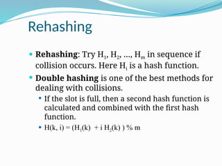
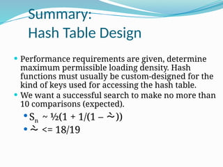
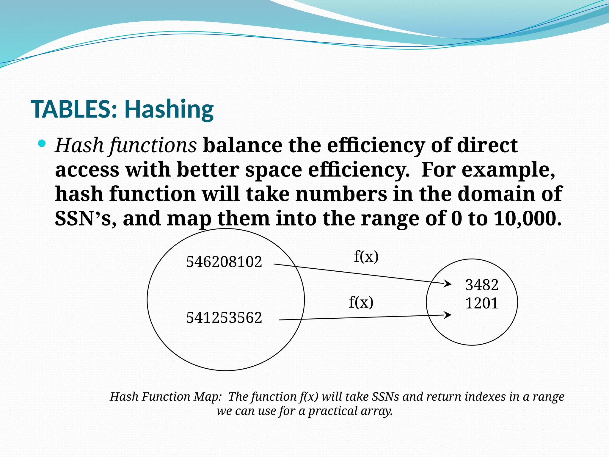
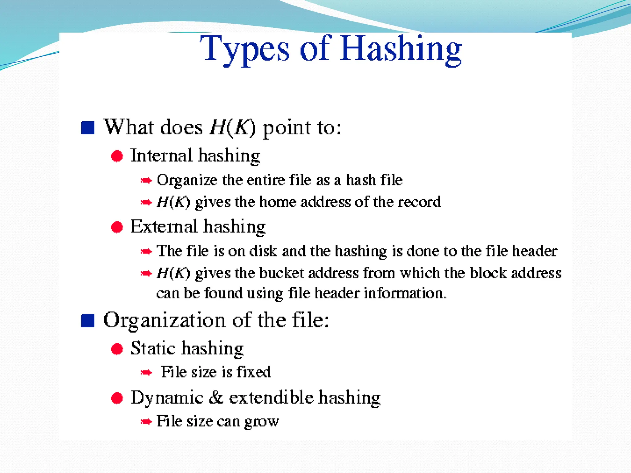
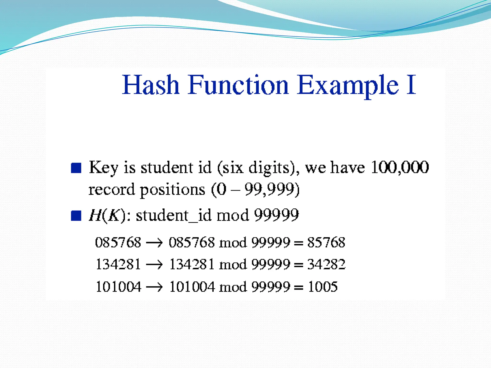
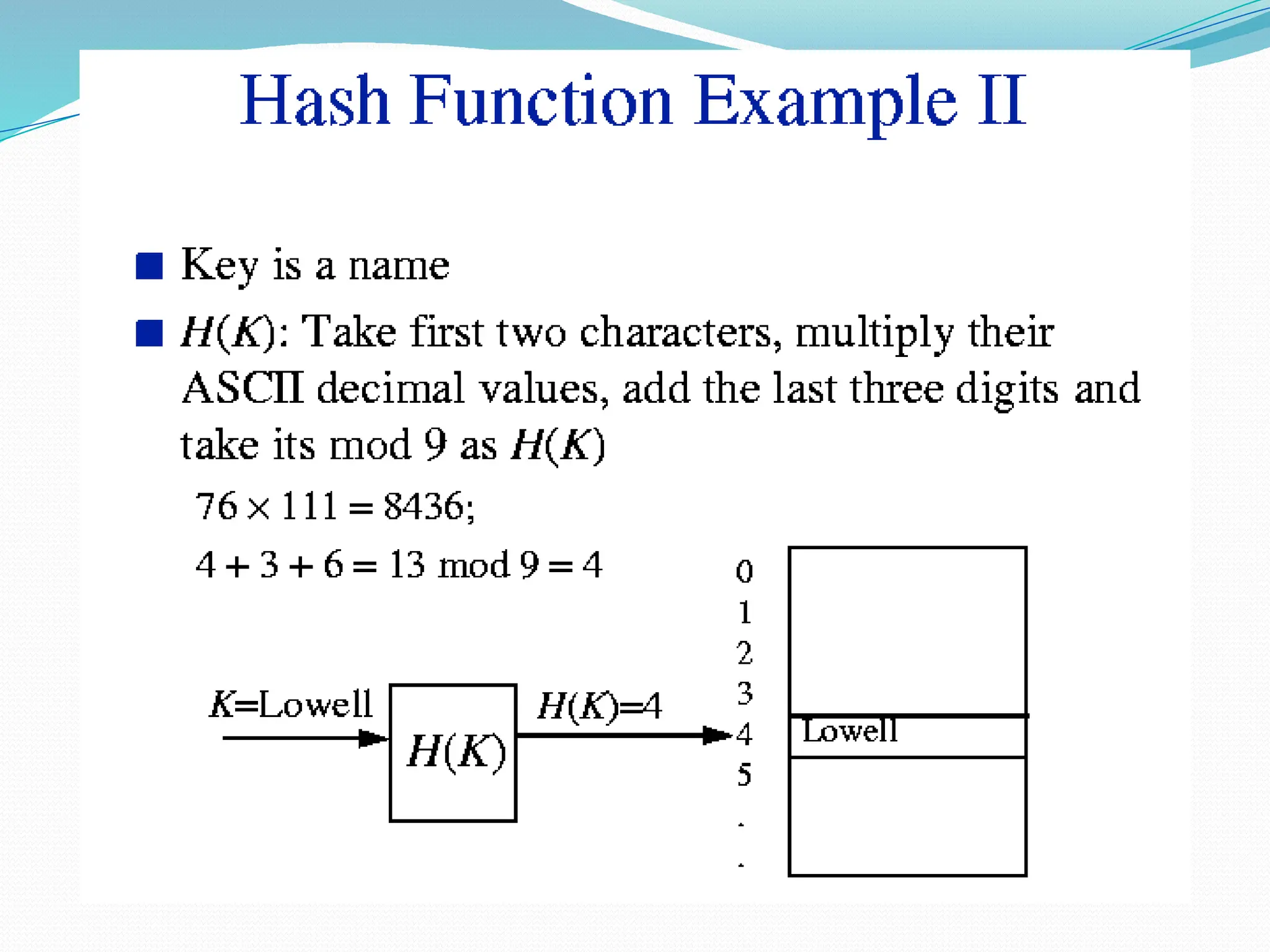
The document discusses hashing, a method for efficiently storing and retrieving data through hash functions that map keys to array indexes. It explains the advantages of hashing over binary search, the structure of hash tables, and various collision resolution strategies like separate chaining and linear probing. Additionally, it covers the design considerations for hash functions and the performance metrics required for effective data access.


![ Suppose we have 50 different stock number
and if the stock numbers have values ranging
from 0 to 49, we could store the records in an
array of the following type, placing stock
number “j” in location data[ j ].
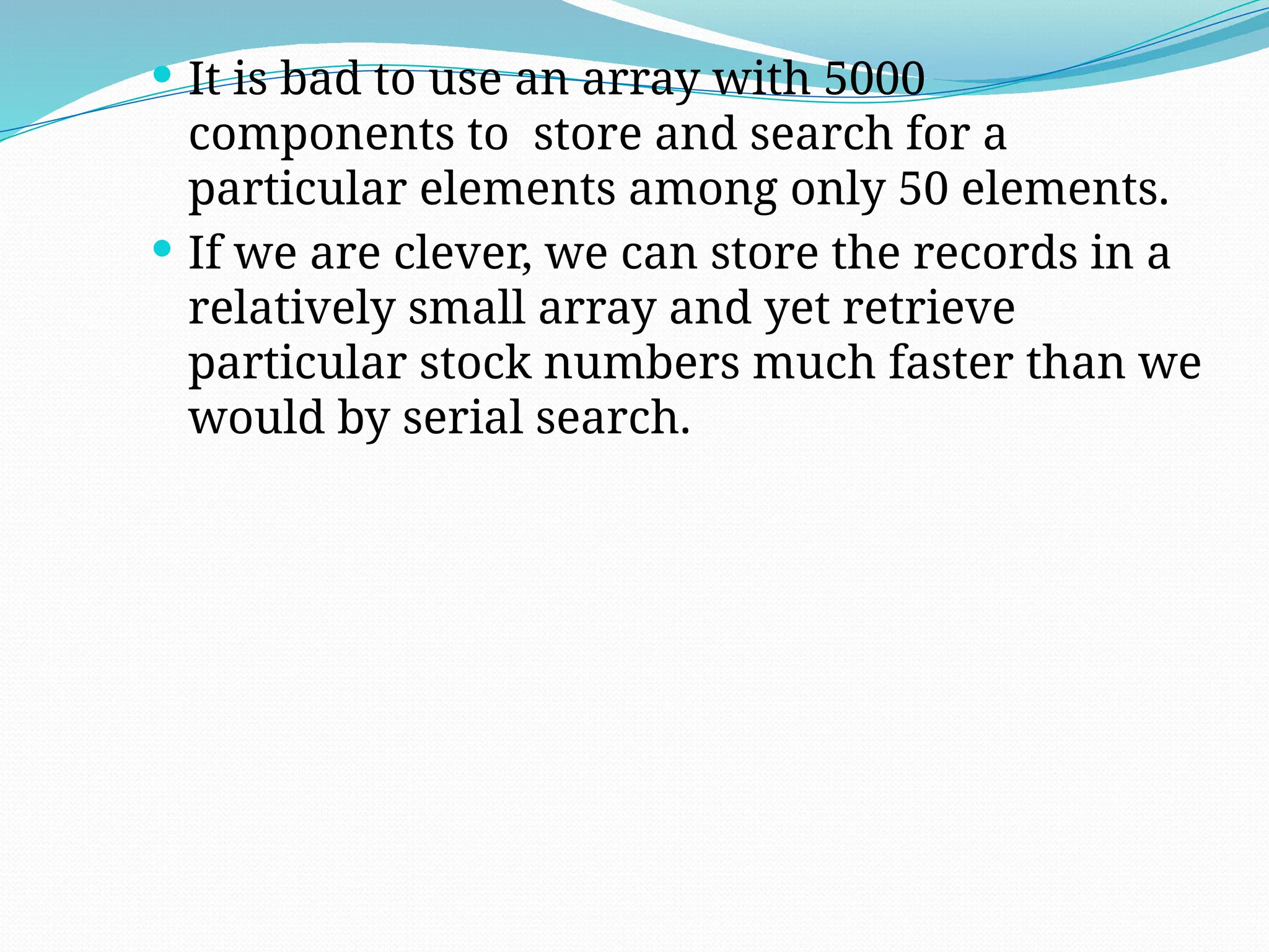
If the stock numbers ranging from 0 to 4999,
we could use an array with 5000 components.
But that seems wasteful since only a small
fraction of array would be used.](https://image.slidesharecdn.com/hashingunit4-250122075111-88307834/85/Hashing_Unit4-pptx-Data-Structures-and-Algos-14-320.jpg)
![ Suppose the stock numbers will be these: 0,
100, 200, 300, … 4800, 4900
In this case we can store the records in an
array called data with only 50 components.
The record with stock number “j” can be
stored at this location:
data[ j / 100]
The record for stock number 4900 is stored in
array component data[49]. This general
technique is called HASHING.](https://image.slidesharecdn.com/hashingunit4-250122075111-88307834/85/Hashing_Unit4-pptx-Data-Structures-and-Algos-16-320.jpg)
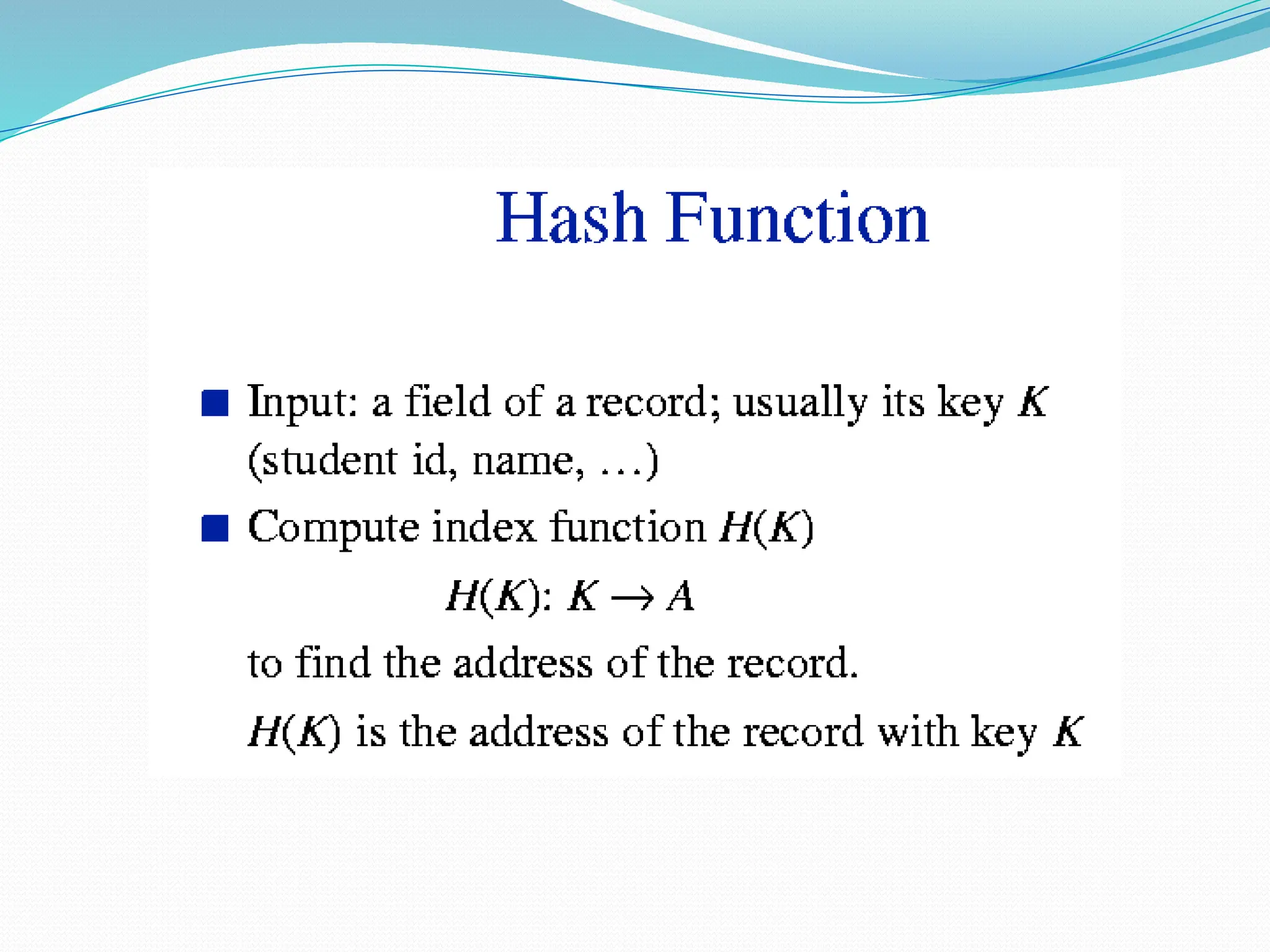
![Key & Hash function
In our example the key was the stock number
that was stored in a member variable called
key.
Hash function maps key values to array
indexes. Suppose we name our hash function
hash.
If a record has the key value of j then we will
try to store the record at location
data[hash(j)], hash(j) was this expression: j /
100](https://image.slidesharecdn.com/hashingunit4-250122075111-88307834/85/Hashing_Unit4-pptx-Data-Structures-and-Algos-17-320.jpg)


![Random Probing
Random Probing works incorporating with
random numbers.
H(x):= (H’(x) + S[i]) % b
S[i] is a table with size b-1
S[i] is a random permuation of integers [1,b-1].](https://image.slidesharecdn.com/hashingunit4-250122075111-88307834/85/Hashing_Unit4-pptx-Data-Structures-and-Algos-44-320.jpg)


![ Suppose we have 50 different stock number
and if the stock numbers have values ranging
from 0 to 49, we could store the records in an
array of the following type, placing stock
number “j” in location data[ j ].
If the stock numbers ranging from 0 to 4999,
we could use an array with 5000 components.
But that seems wasteful since only a small
fraction of array would be used.](https://image.slidesharecdn.com/hashingunit4-250122075111-88307834/75/Hashing_Unit4-pptx-Data-Structures-and-Algos-14-2048.jpg)
![ Suppose the stock numbers will be these: 0,
100, 200, 300, … 4800, 4900
In this case we can store the records in an
array called data with only 50 components.
The record with stock number “j” can be
stored at this location:
data[ j / 100]
The record for stock number 4900 is stored in
array component data[49]. This general
technique is called HASHING.](https://image.slidesharecdn.com/hashingunit4-250122075111-88307834/75/Hashing_Unit4-pptx-Data-Structures-and-Algos-16-2048.jpg)
![Key & Hash function
In our example the key was the stock number
that was stored in a member variable called
key.
Hash function maps key values to array
indexes. Suppose we name our hash function
hash.
If a record has the key value of j then we will
try to store the record at location
data[hash(j)], hash(j) was this expression: j /
100](https://image.slidesharecdn.com/hashingunit4-250122075111-88307834/75/Hashing_Unit4-pptx-Data-Structures-and-Algos-17-2048.jpg)


![Random Probing
Random Probing works incorporating with
random numbers.
H(x):= (H’(x) + S[i]) % b
S[i] is a table with size b-1
S[i] is a random permuation of integers [1,b-1].](https://image.slidesharecdn.com/hashingunit4-250122075111-88307834/75/Hashing_Unit4-pptx-Data-Structures-and-Algos-44-2048.jpg)