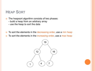
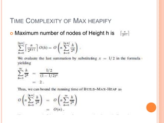
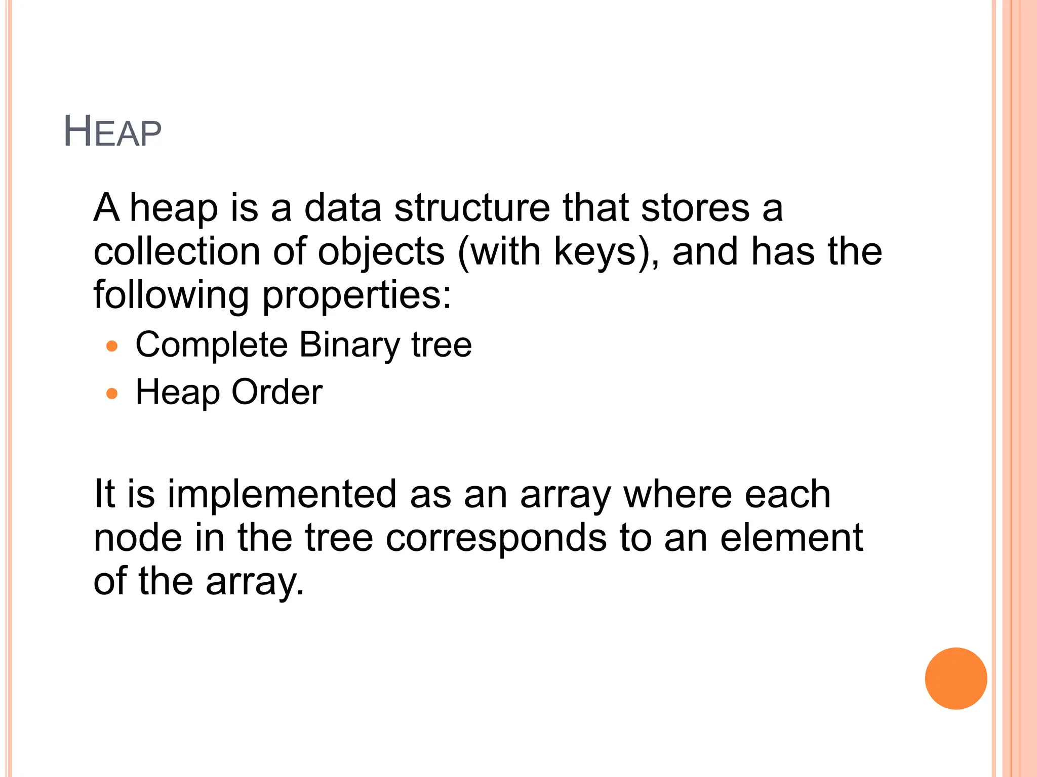
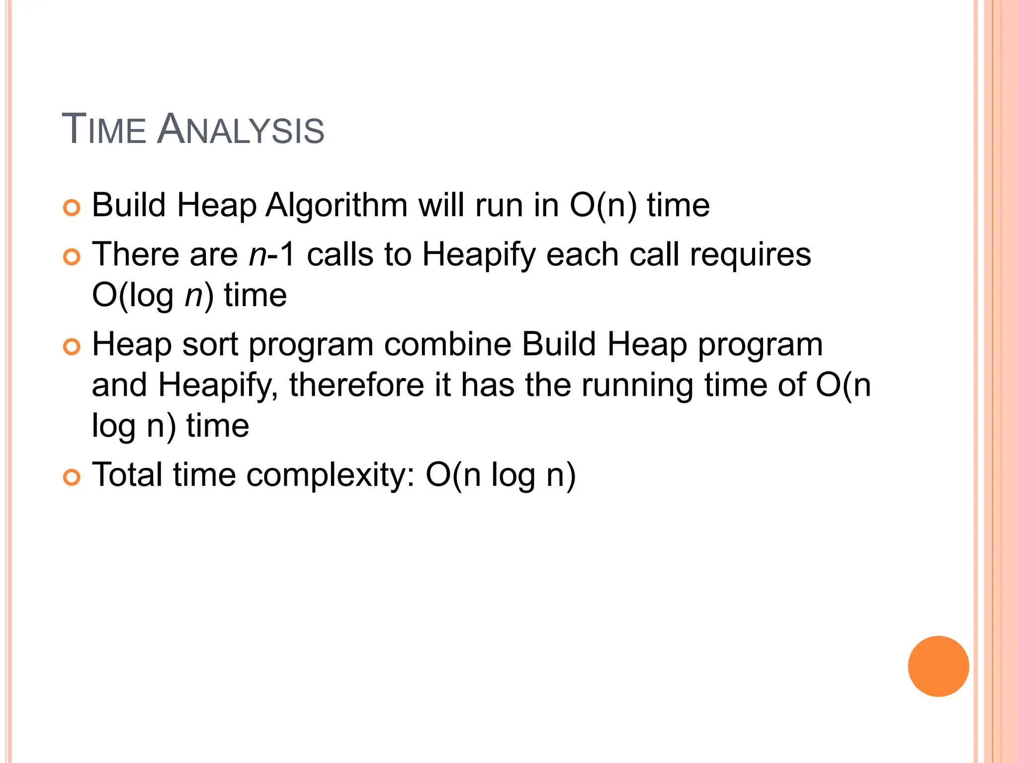
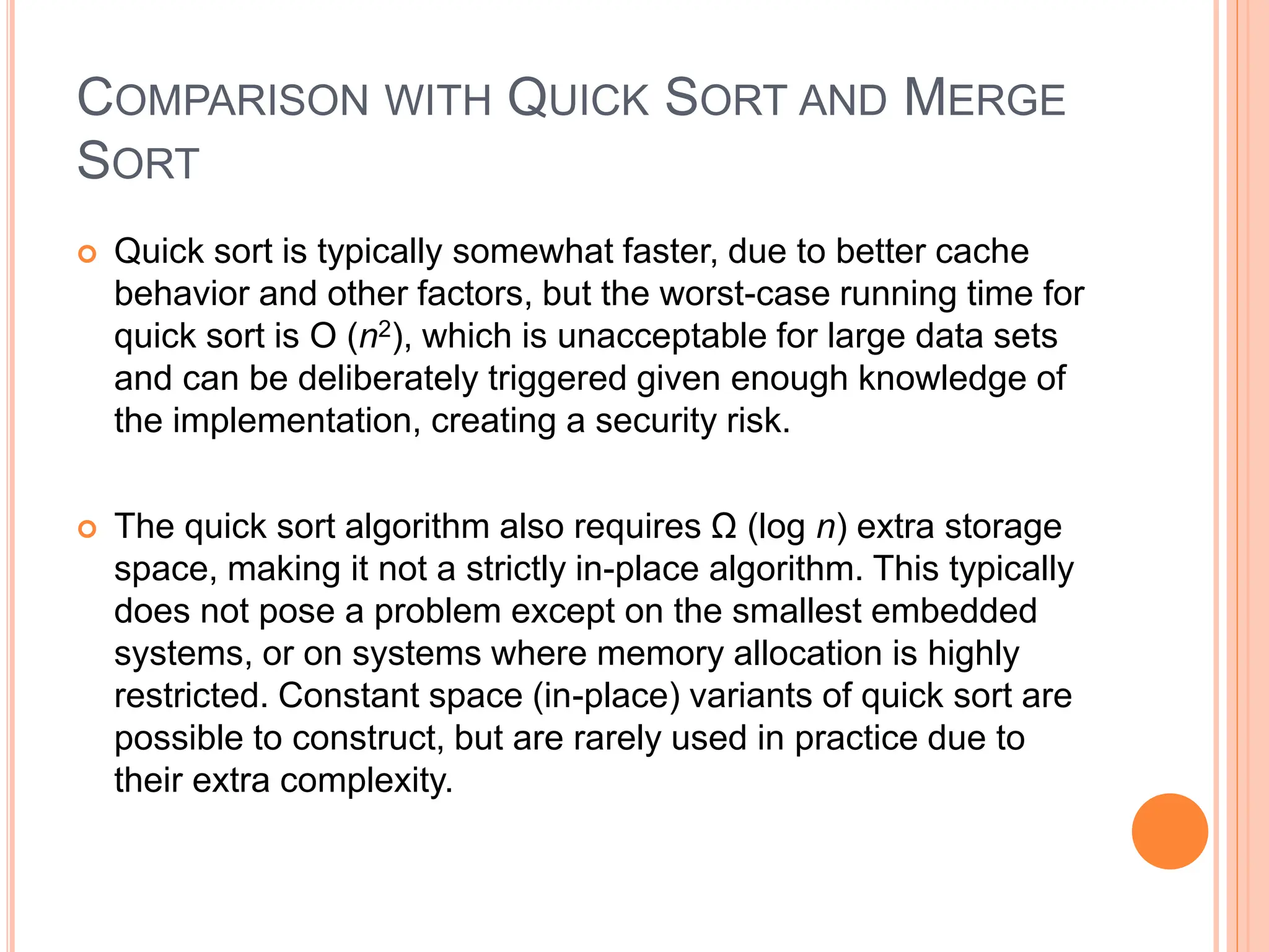
Heap sort is a sorting algorithm that uses a heap data structure. It works in two phases: first it builds a max heap from the input data, then it repeatedly extracts the largest element from the heap and inserts it into the sorted end of the data. This results in the elements being sorted in O(n log n) time using only O(1) additional memory space, making it efficient for both time and space complexity. It performs better than quicksort in the worst case but requires random access to data unlike merge sort.


![HEAP
The root of the tree A[1] and given index i of a
node, the indices of its parent, left child and right
child can be computed
PARENT (i)
return floor(i/2)
LEFT (i)
return 2i
RIGHT (i)
return 2i + 1](https://image.slidesharecdn.com/heapsortproject-240227040436-7ed22815/85/heap-sort-in-the-design-anad-analysis-of-algorithms-4-320.jpg)
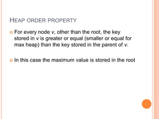
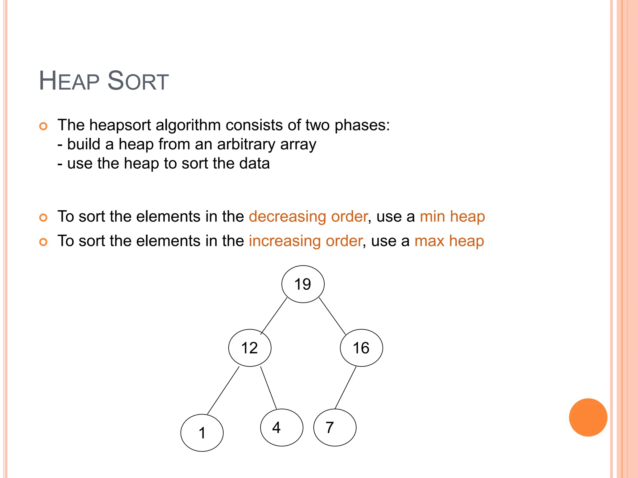
![DEFINITION
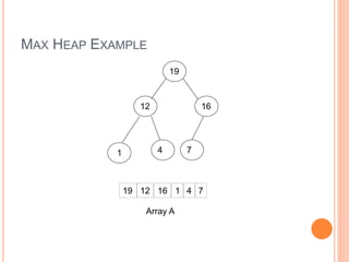
Max Heap
Store data in ascending order
Has property of
A[Parent(i)] ≥ A[i]
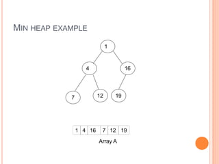
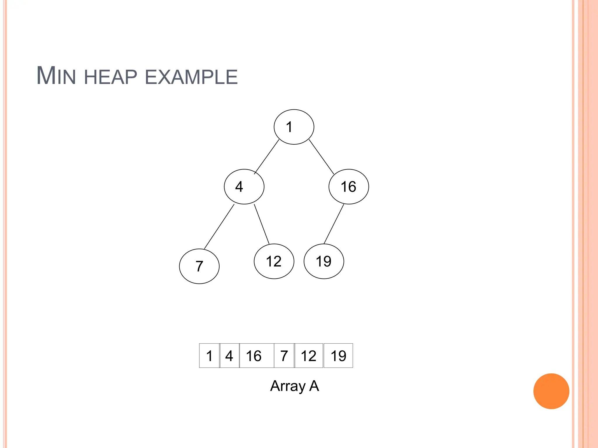
Min Heap
Store data in descending order
Has property of
A[Parent(i)] ≤ A[i]](https://image.slidesharecdn.com/heapsortproject-240227040436-7ed22815/85/heap-sort-in-the-design-anad-analysis-of-algorithms-6-320.jpg)


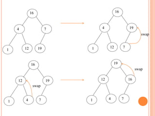
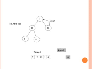
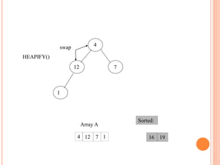
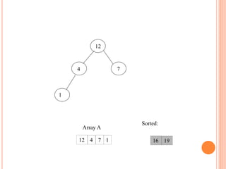
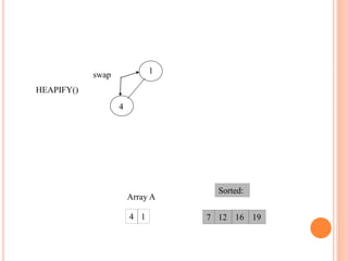
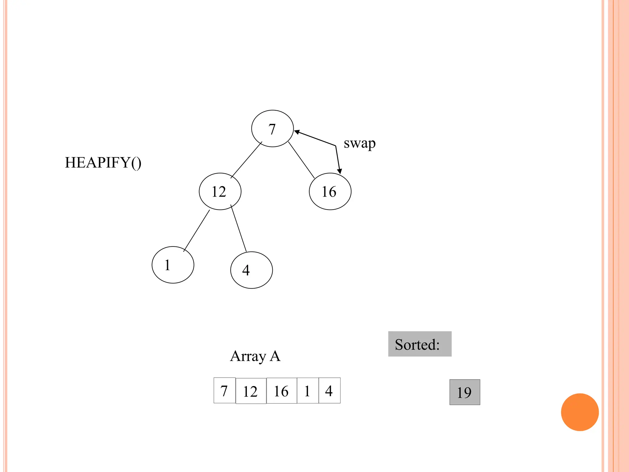
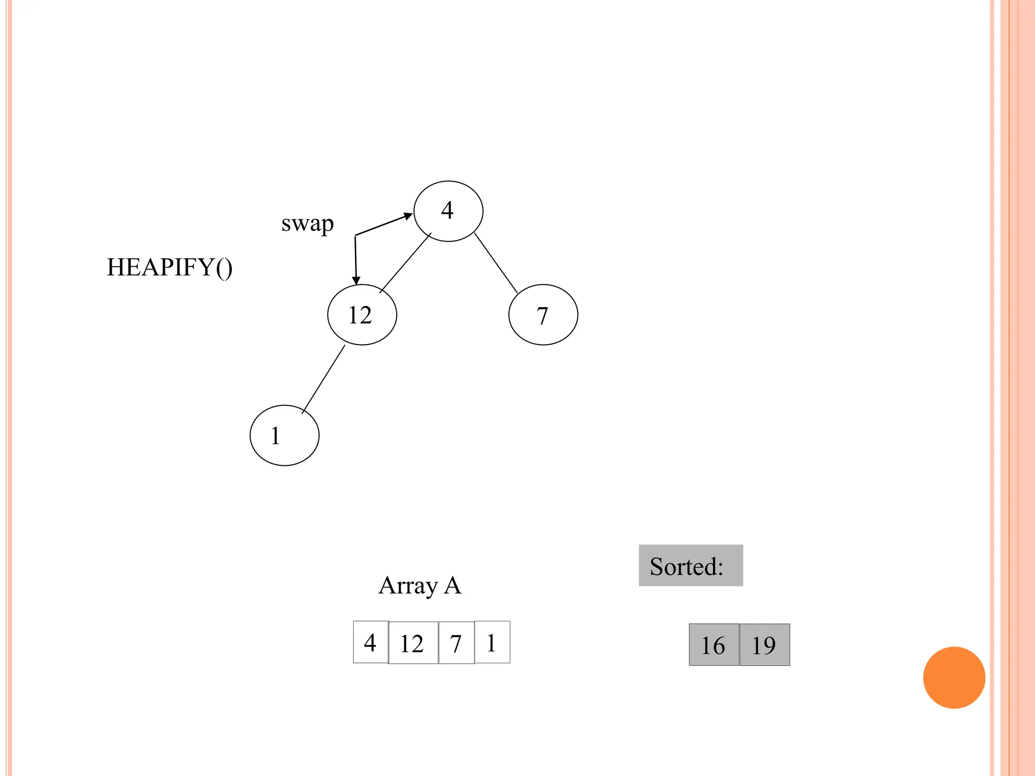
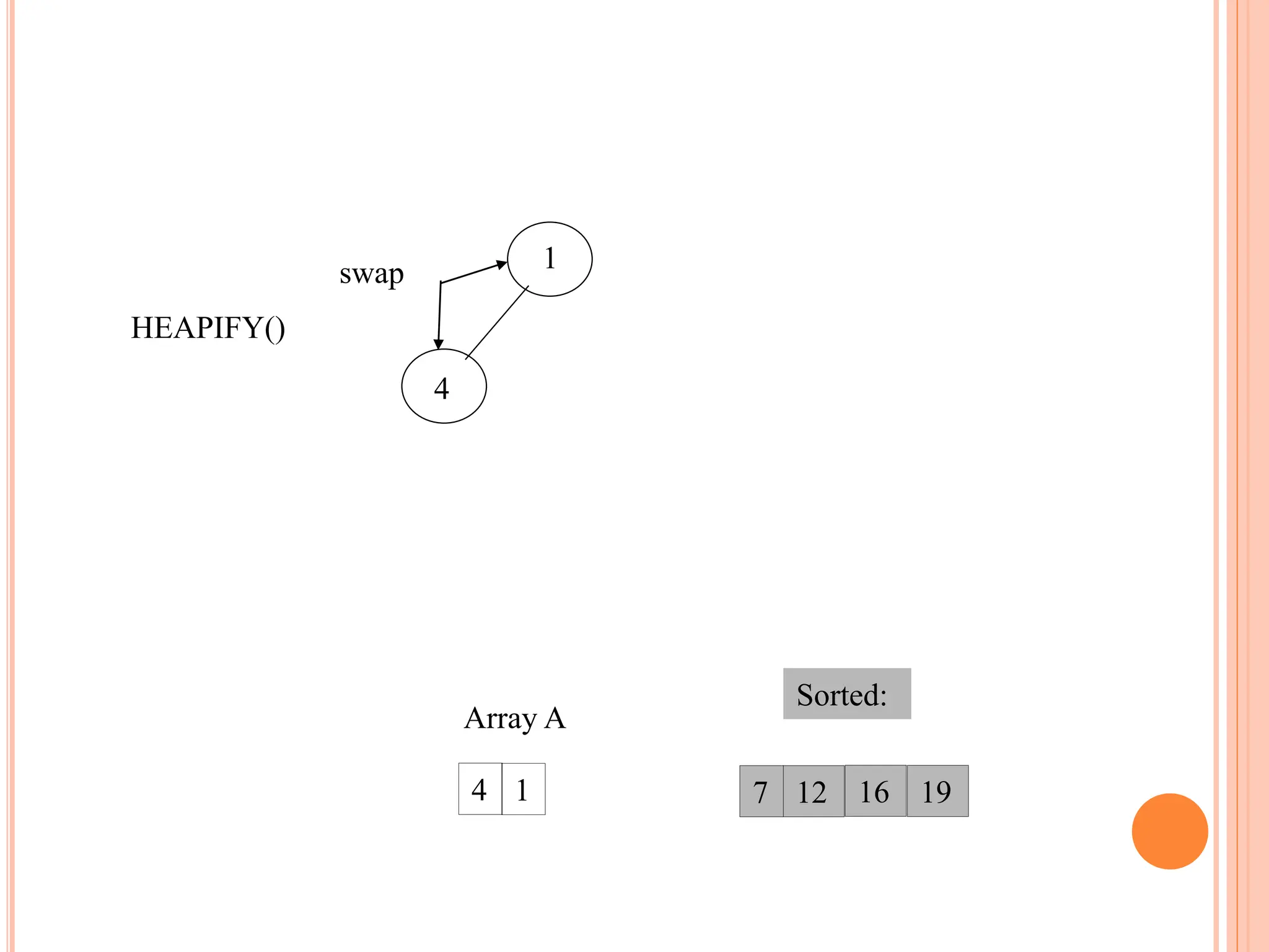
![HEAPIFY
Heapify picks the largest child key and compare it to the
parent key. If parent key is larger than heapify quits, otherwise
it swaps the parent key with the largest child key. So that the
parent is now becomes larger than its children.
Heapify(A, i)
{
l left(i)
r right(i)
if l <= heapsize[A] and A[l] > A[i]
then largest l
else largest i
if r <= heapsize[A] and A[r] > A[largest]
then largest r
if largest != i
then swap A[i] A[largest]
Heapify(A, largest)
}](https://image.slidesharecdn.com/heapsortproject-240227040436-7ed22815/85/heap-sort-in-the-design-anad-analysis-of-algorithms-14-320.jpg)
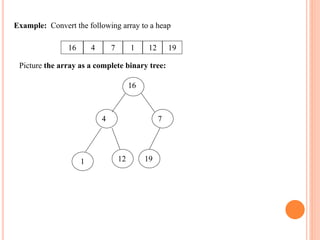
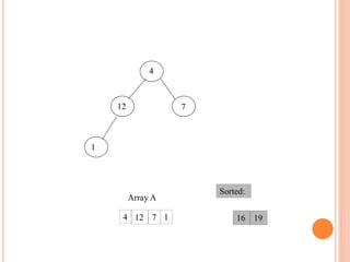
![BUILD HEAP
We can use the procedure 'Heapify' in a bottom-up fashion to
convert an array A[1 . . n] into a heap. Since the elements in
the subarray A[n/2 +1 . . n] are all leaves, the procedure
BUILD_HEAP goes through the remaining nodes of the tree
and runs 'Heapify' on each one. The bottom-up order of
processing node guarantees that the subtree rooted at
children are heap before 'Heapify' is run at their parent.
Buildheap(A)
{
heapsize[A] length[A]
for i |length[A]/2 //down to 1
do Heapify(A, i)
}](https://image.slidesharecdn.com/heapsortproject-240227040436-7ed22815/85/heap-sort-in-the-design-anad-analysis-of-algorithms-15-320.jpg)
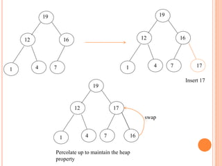
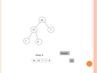
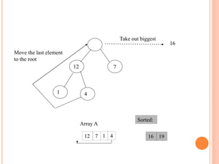
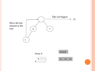
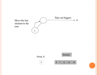
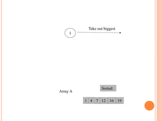
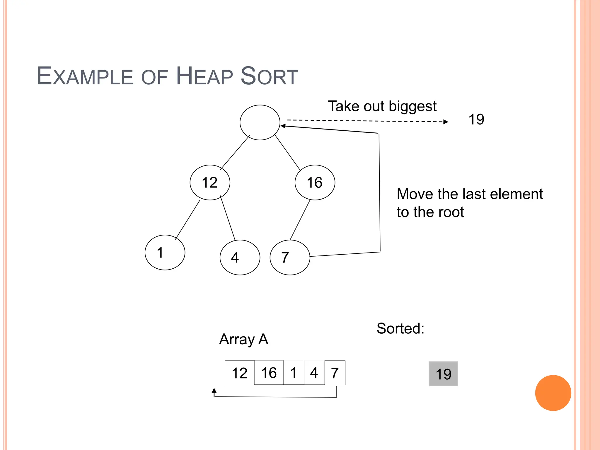
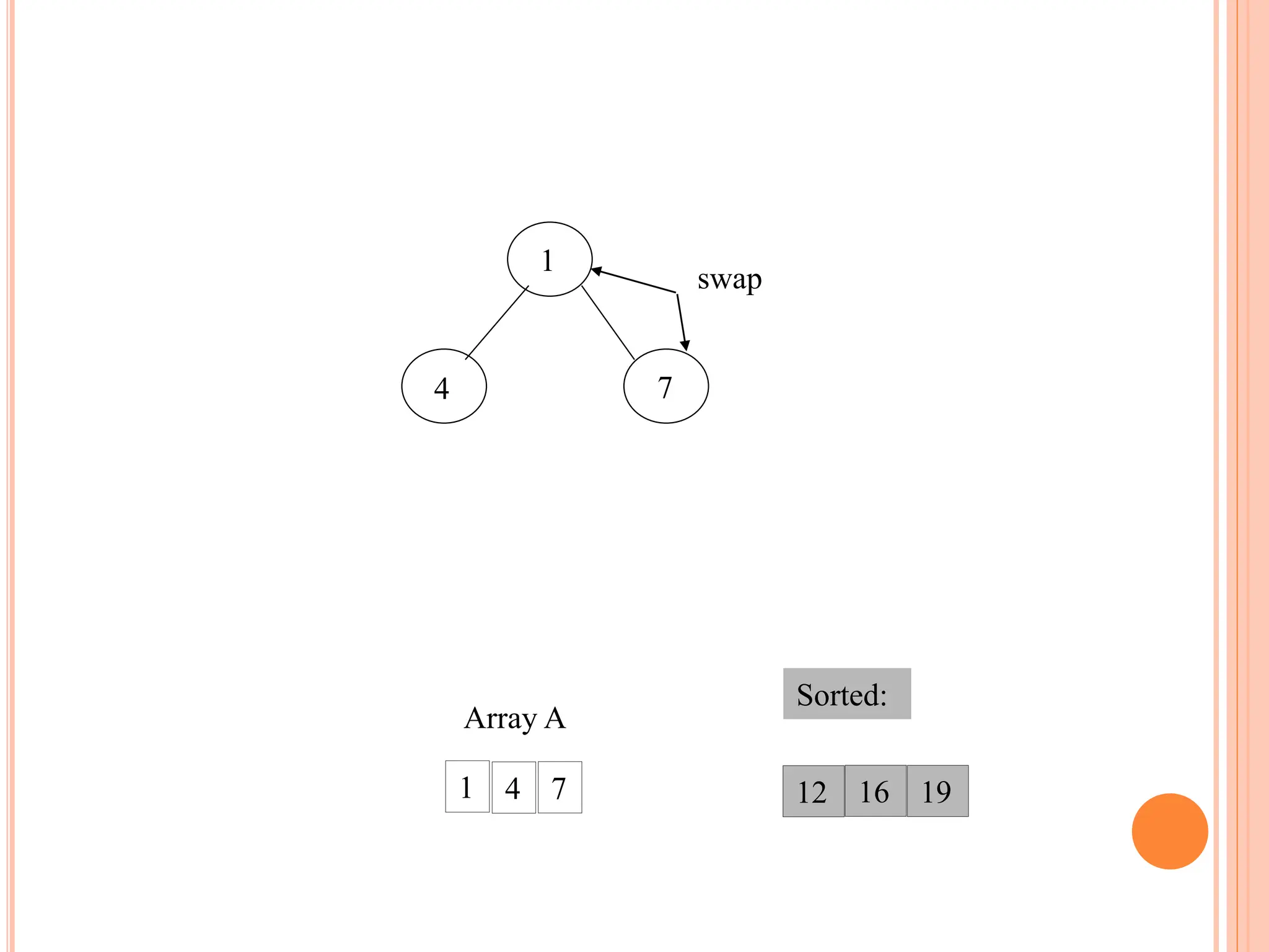
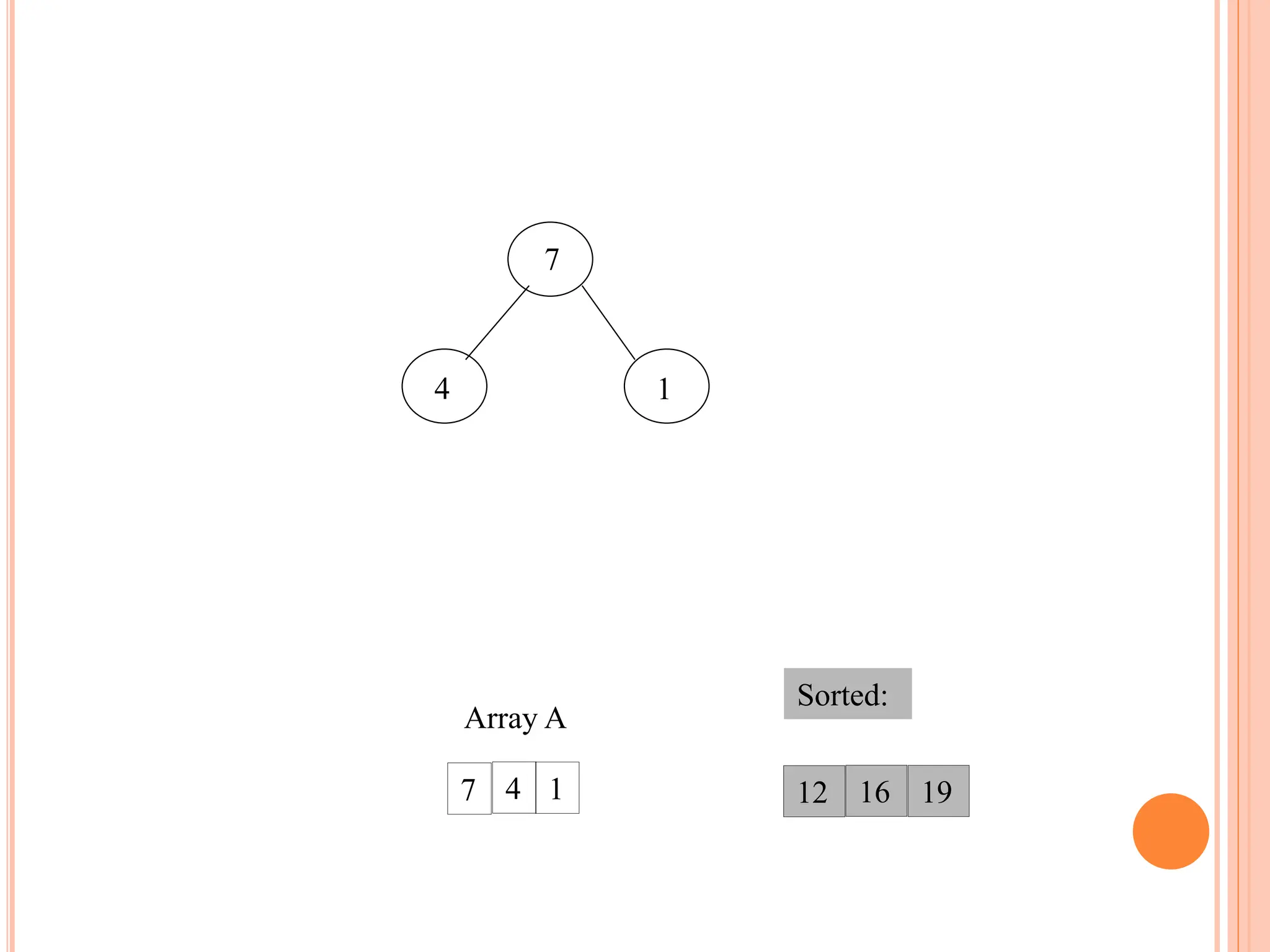
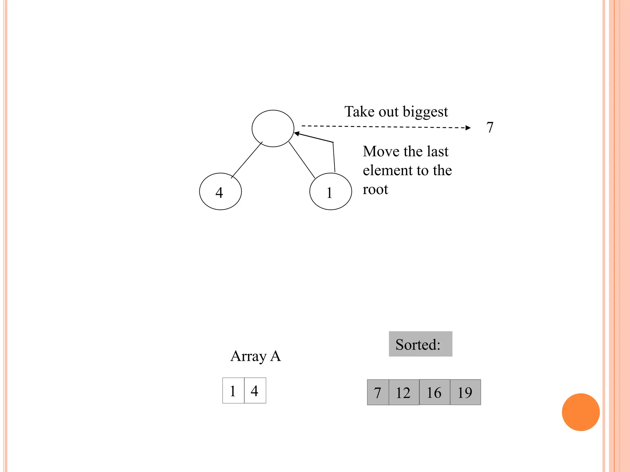
![HEAP SORT ALGORITHM
The heap sort algorithm starts by using procedure BUILD-
HEAP to build a heap on the input array A[1 . . n]. Since the
maximum element of the array stored at the root A[1], it can
be put into its correct final position by exchanging it with A[n]
(the last element in A). If we now discard node n from the
heap than the remaining elements can be made into heap.
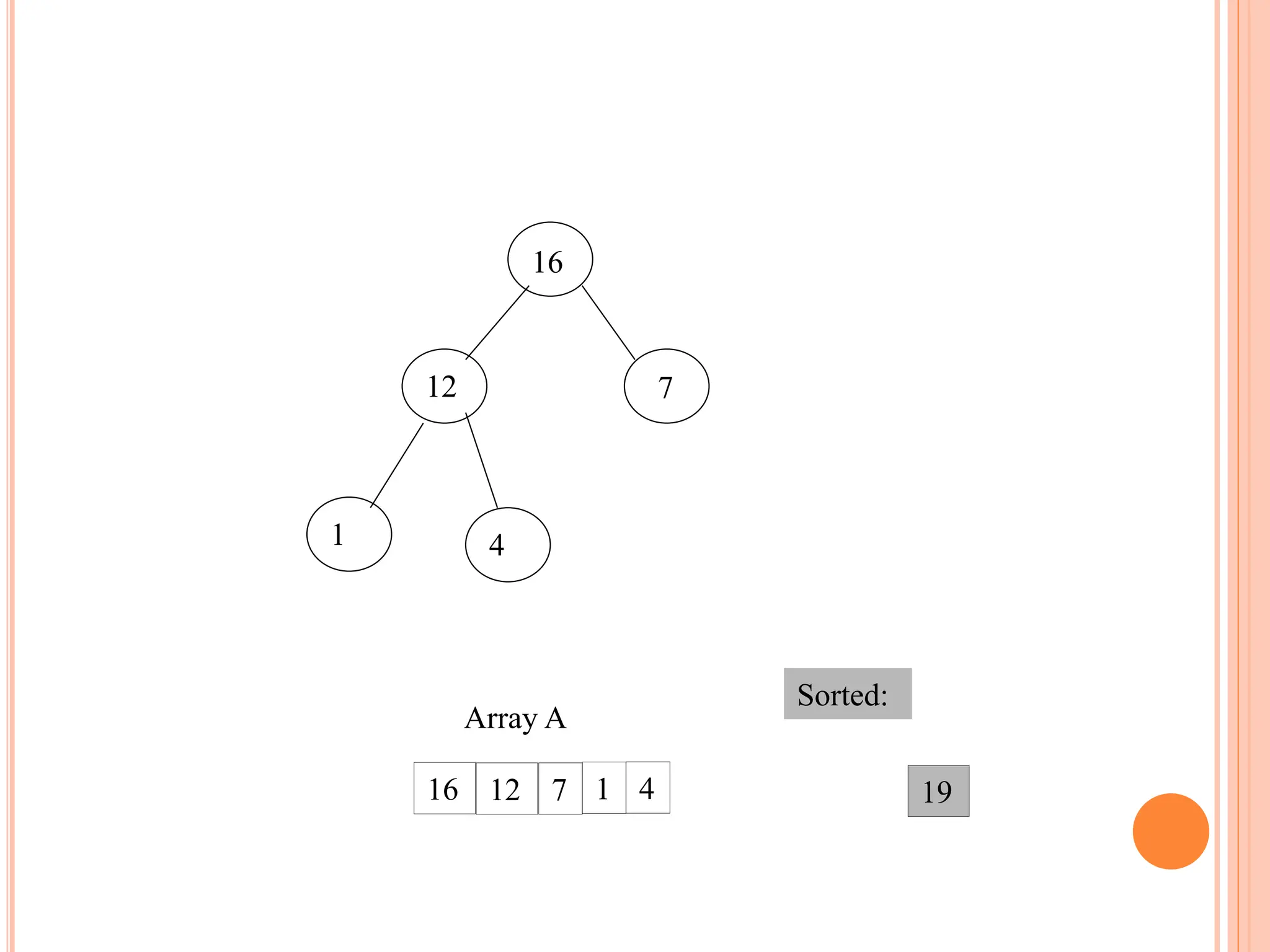
Note that the new element at the root may violate the heap
property. All that is needed to restore the heap property.
Heapsort(A)
{
Buildheap(A)
for i length[A] //down to 2
do swap A[1] A[i]
heapsize[A] heapsize[A] - 1
Heapify(A, 1)
}](https://image.slidesharecdn.com/heapsortproject-240227040436-7ed22815/85/heap-sort-in-the-design-anad-analysis-of-algorithms-16-320.jpg)


![HEAP
The root of the tree A[1] and given index i of a
node, the indices of its parent, left child and right
child can be computed
PARENT (i)
return floor(i/2)
LEFT (i)
return 2i
RIGHT (i)
return 2i + 1](https://image.slidesharecdn.com/heapsortproject-240227040436-7ed22815/75/heap-sort-in-the-design-anad-analysis-of-algorithms-4-2048.jpg)
![DEFINITION
Max Heap
Store data in ascending order
Has property of
A[Parent(i)] ≥ A[i]
Min Heap
Store data in descending order
Has property of
A[Parent(i)] ≤ A[i]](https://image.slidesharecdn.com/heapsortproject-240227040436-7ed22815/75/heap-sort-in-the-design-anad-analysis-of-algorithms-6-2048.jpg)
![HEAPIFY
Heapify picks the largest child key and compare it to the
parent key. If parent key is larger than heapify quits, otherwise
it swaps the parent key with the largest child key. So that the
parent is now becomes larger than its children.
Heapify(A, i)
{
l left(i)
r right(i)
if l <= heapsize[A] and A[l] > A[i]
then largest l
else largest i
if r <= heapsize[A] and A[r] > A[largest]
then largest r
if largest != i
then swap A[i] A[largest]
Heapify(A, largest)
}](https://image.slidesharecdn.com/heapsortproject-240227040436-7ed22815/75/heap-sort-in-the-design-anad-analysis-of-algorithms-14-2048.jpg)
![BUILD HEAP
We can use the procedure 'Heapify' in a bottom-up fashion to
convert an array A[1 . . n] into a heap. Since the elements in
the subarray A[n/2 +1 . . n] are all leaves, the procedure
BUILD_HEAP goes through the remaining nodes of the tree
and runs 'Heapify' on each one. The bottom-up order of
processing node guarantees that the subtree rooted at
children are heap before 'Heapify' is run at their parent.
Buildheap(A)
{
heapsize[A] length[A]
for i |length[A]/2 //down to 1
do Heapify(A, i)
}](https://image.slidesharecdn.com/heapsortproject-240227040436-7ed22815/75/heap-sort-in-the-design-anad-analysis-of-algorithms-15-2048.jpg)
![HEAP SORT ALGORITHM
The heap sort algorithm starts by using procedure BUILD-
HEAP to build a heap on the input array A[1 . . n]. Since the
maximum element of the array stored at the root A[1], it can
be put into its correct final position by exchanging it with A[n]
(the last element in A). If we now discard node n from the
heap than the remaining elements can be made into heap.
Note that the new element at the root may violate the heap
property. All that is needed to restore the heap property.
Heapsort(A)
{
Buildheap(A)
for i length[A] //down to 2
do swap A[1] A[i]
heapsize[A] heapsize[A] - 1
Heapify(A, 1)
}](https://image.slidesharecdn.com/heapsortproject-240227040436-7ed22815/75/heap-sort-in-the-design-anad-analysis-of-algorithms-16-2048.jpg)


![Depth first search [dfs]](https://cdn.slidesharecdn.com/ss_thumbnails/depthfirstsearchdfs-190926145304-thumbnail.jpg?width=600ounds&width=560&fit=bounds)


