Download as PPS, PPTX
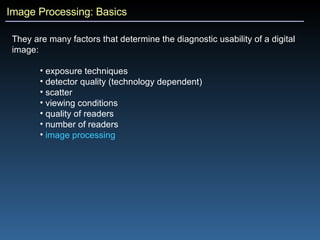


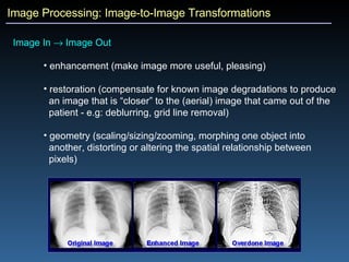

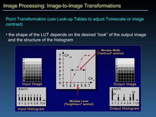
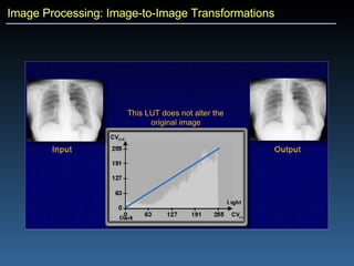
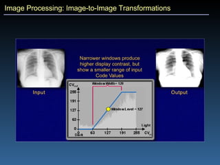
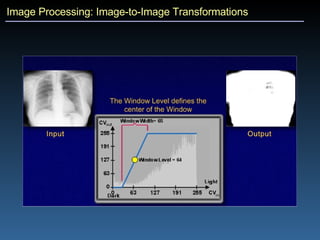
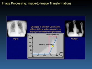
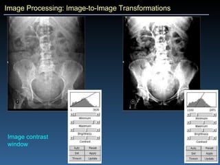
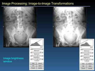

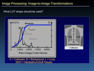
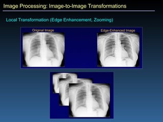
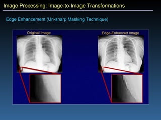
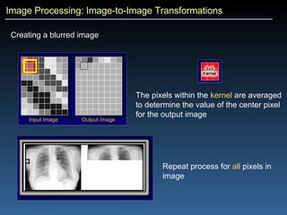

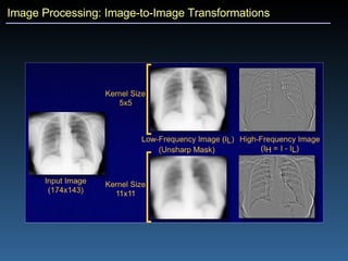
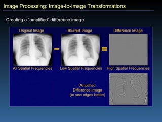
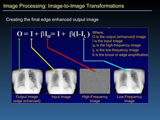
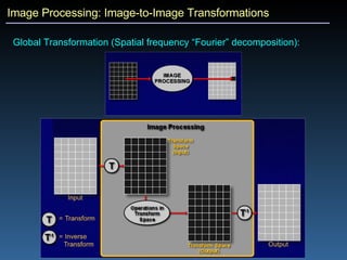
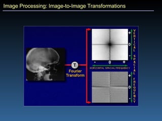
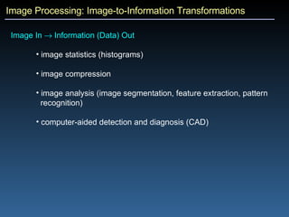
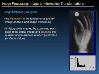
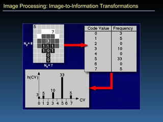
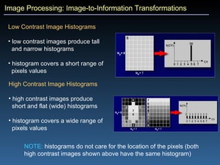
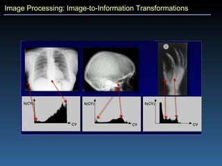

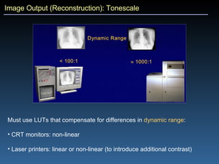
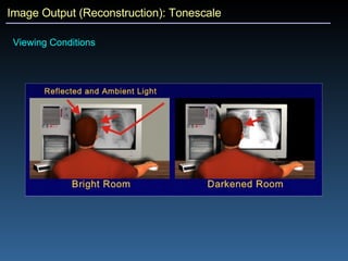
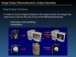
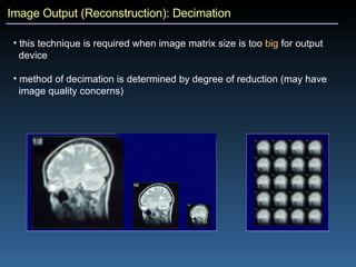

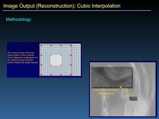
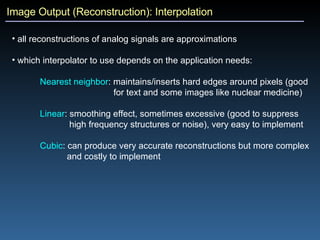
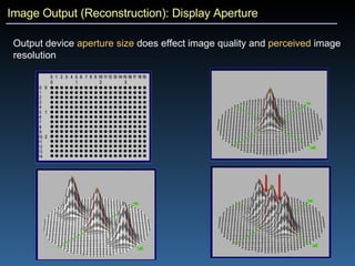


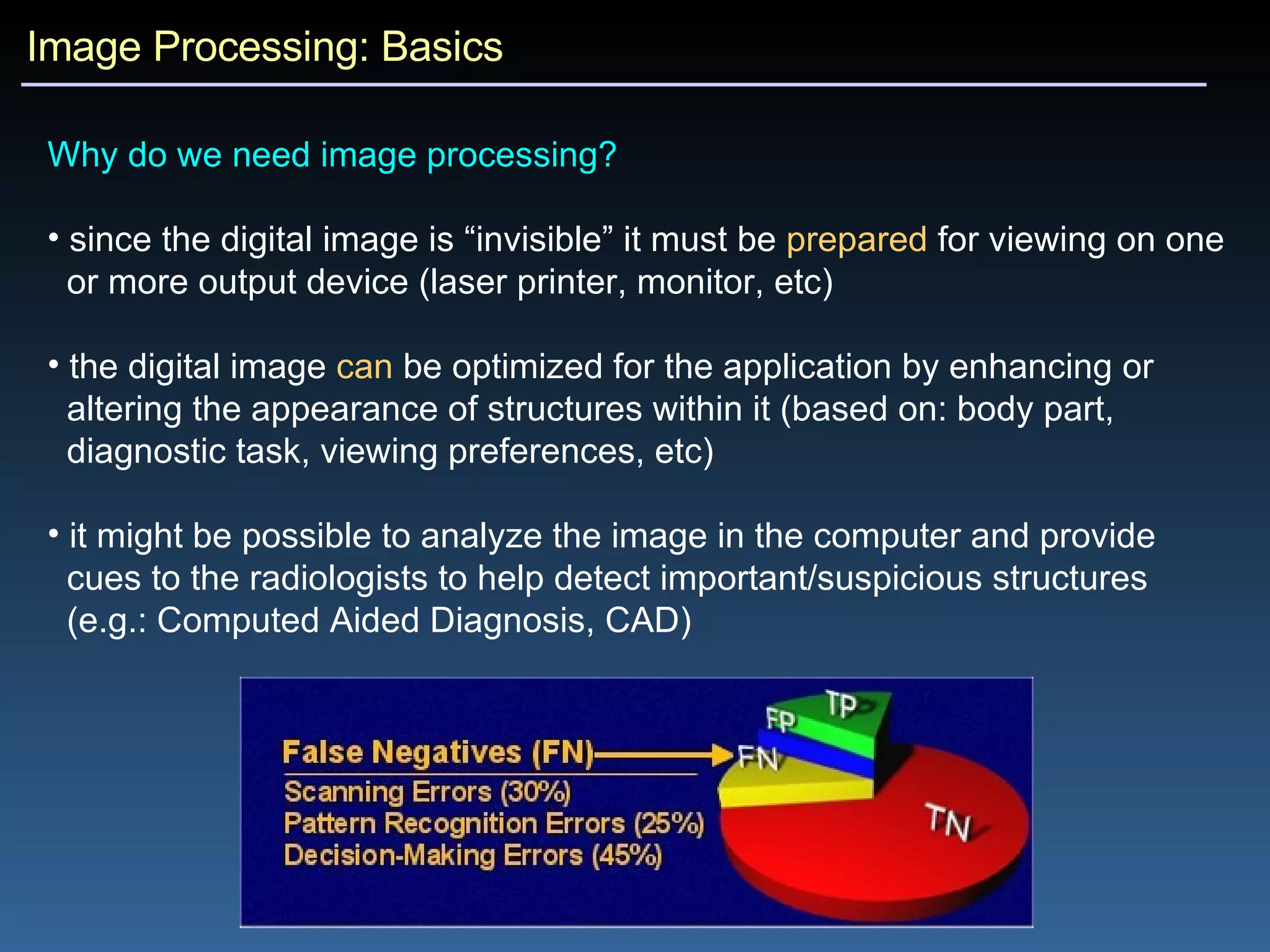
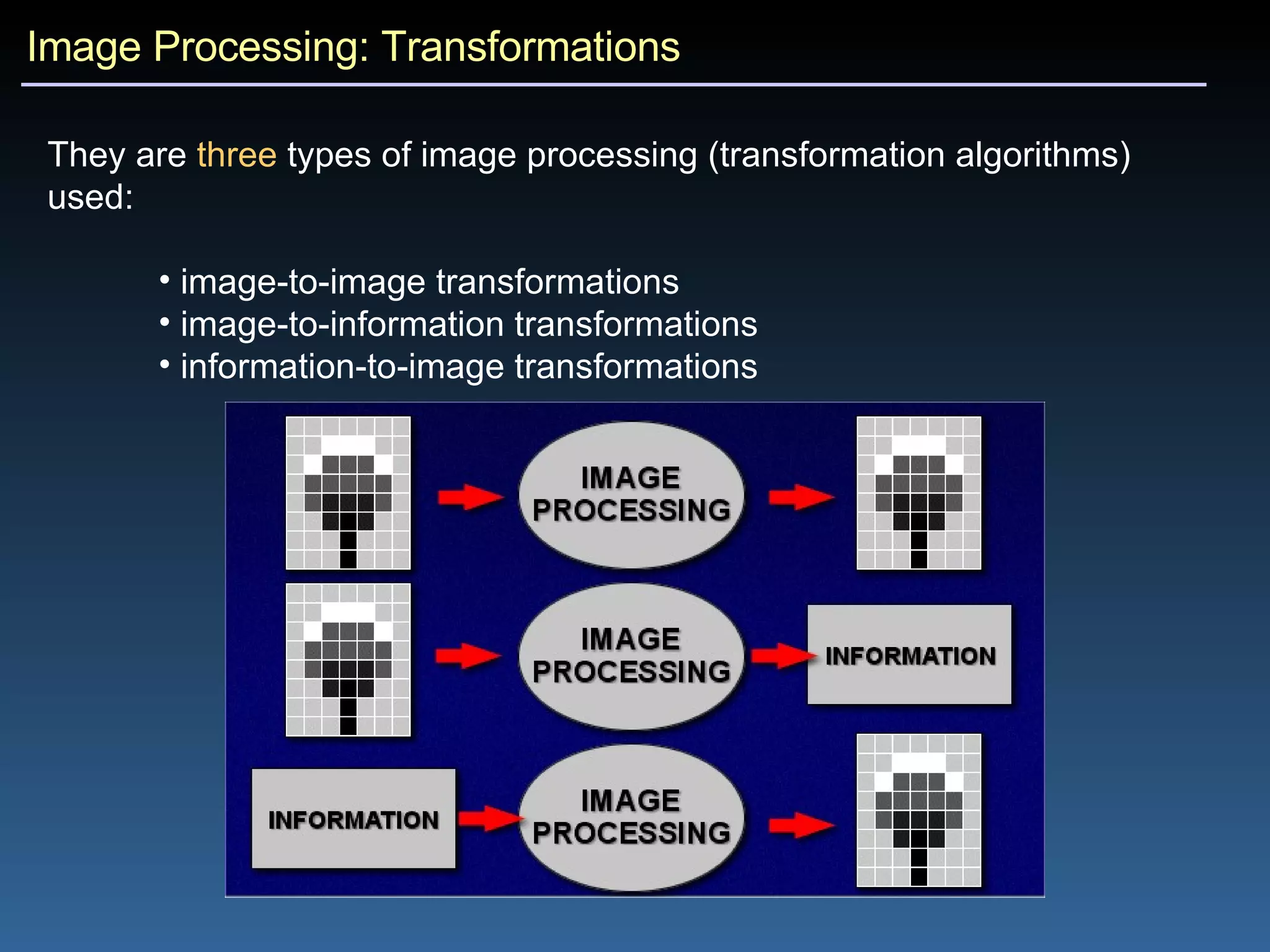
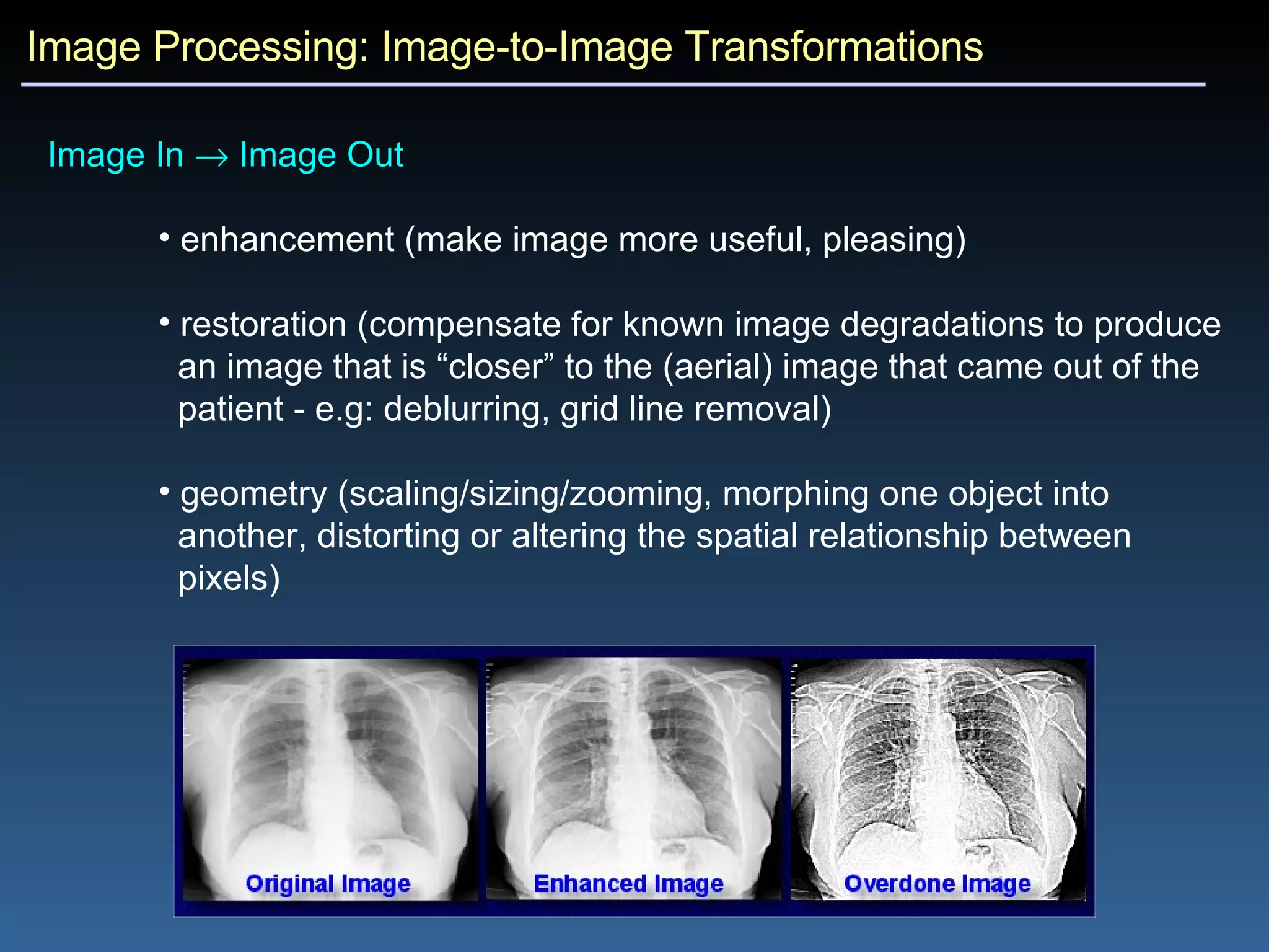
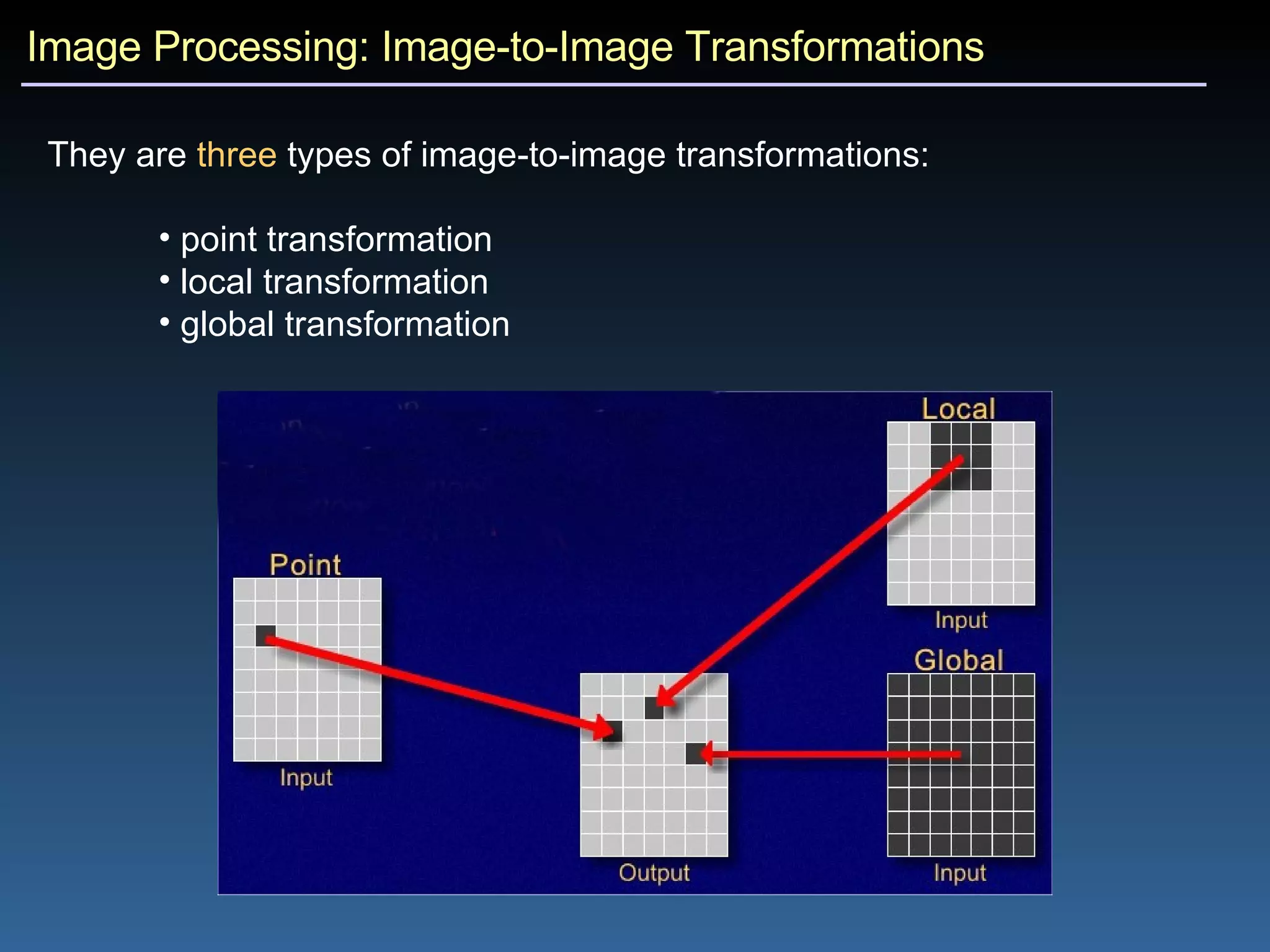
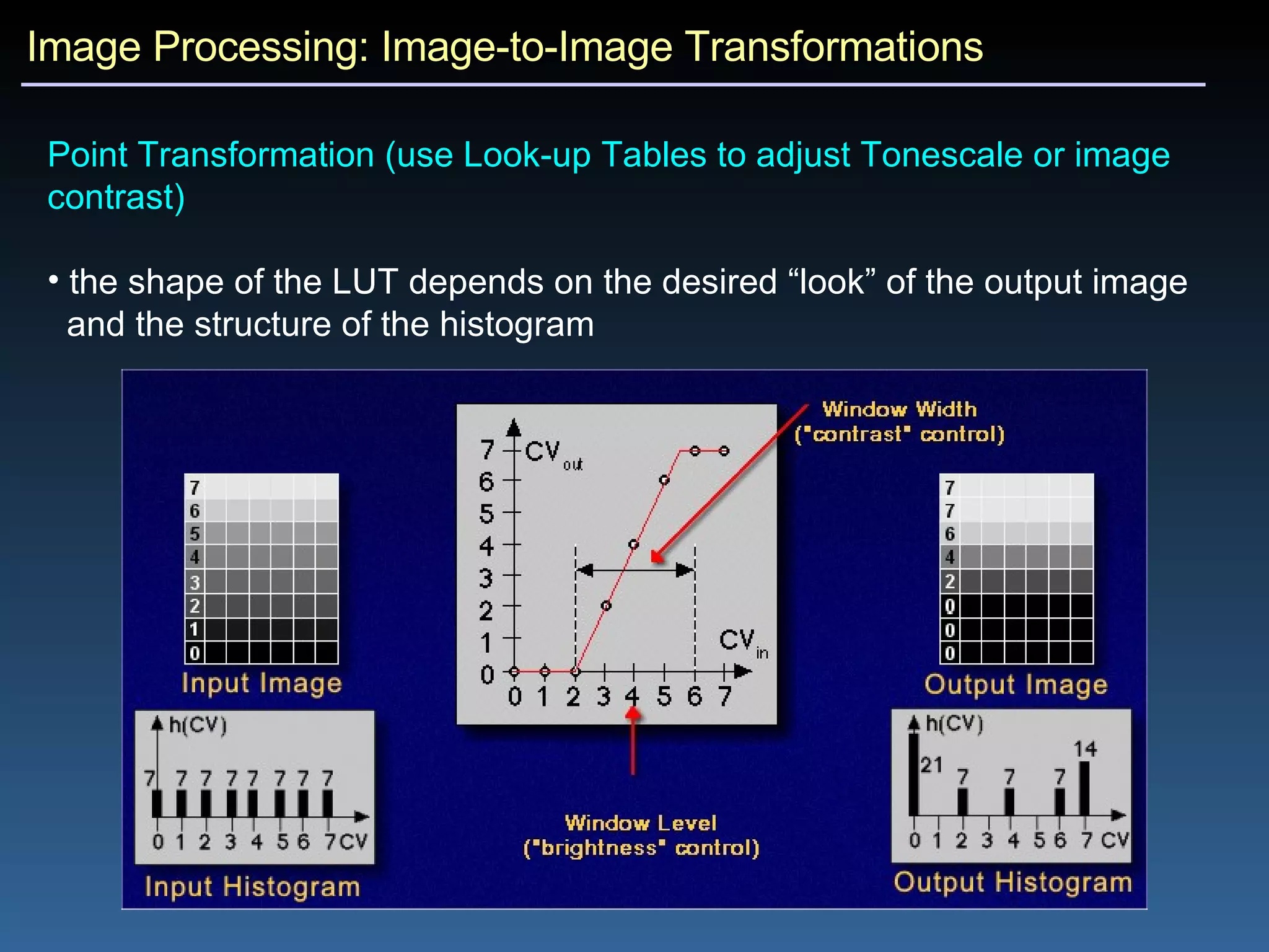

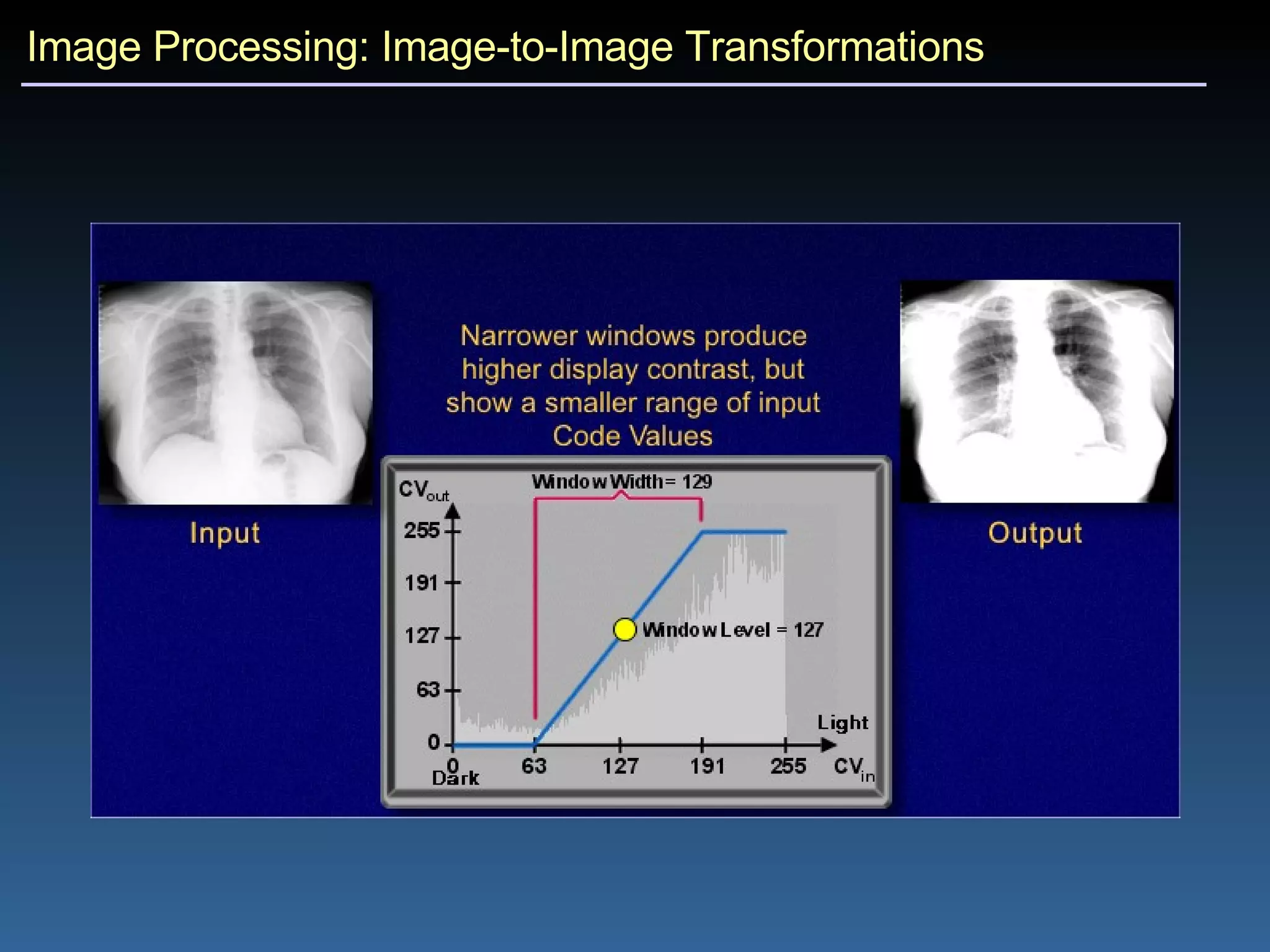
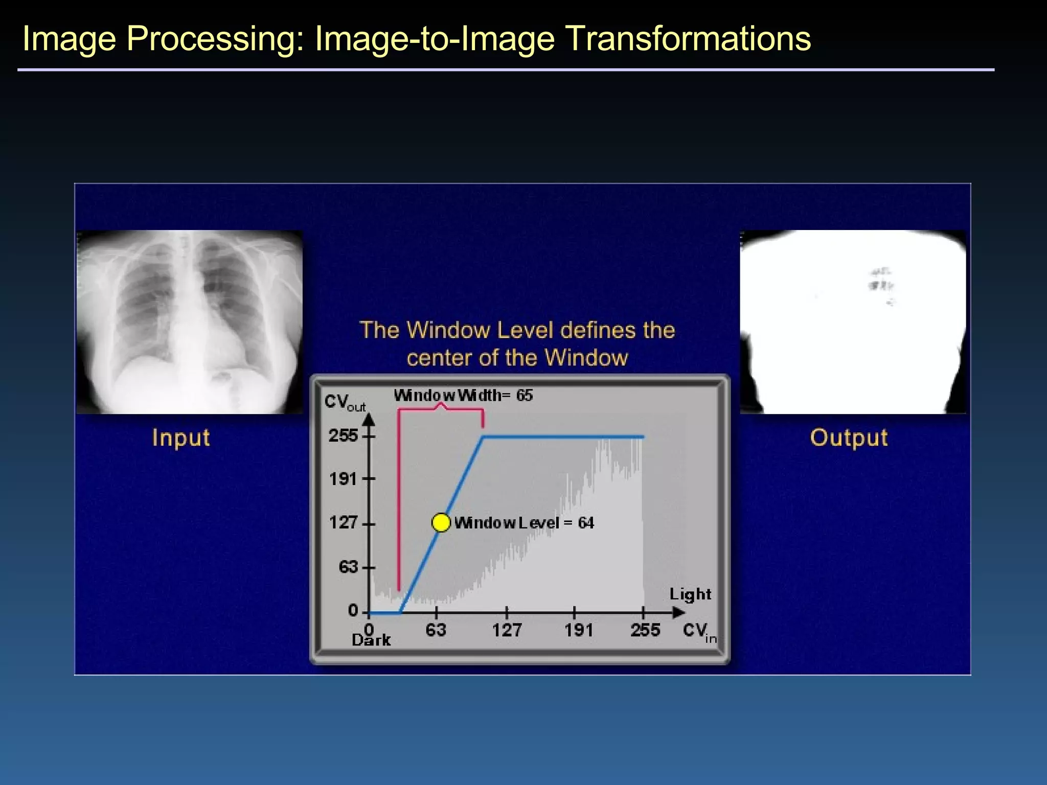
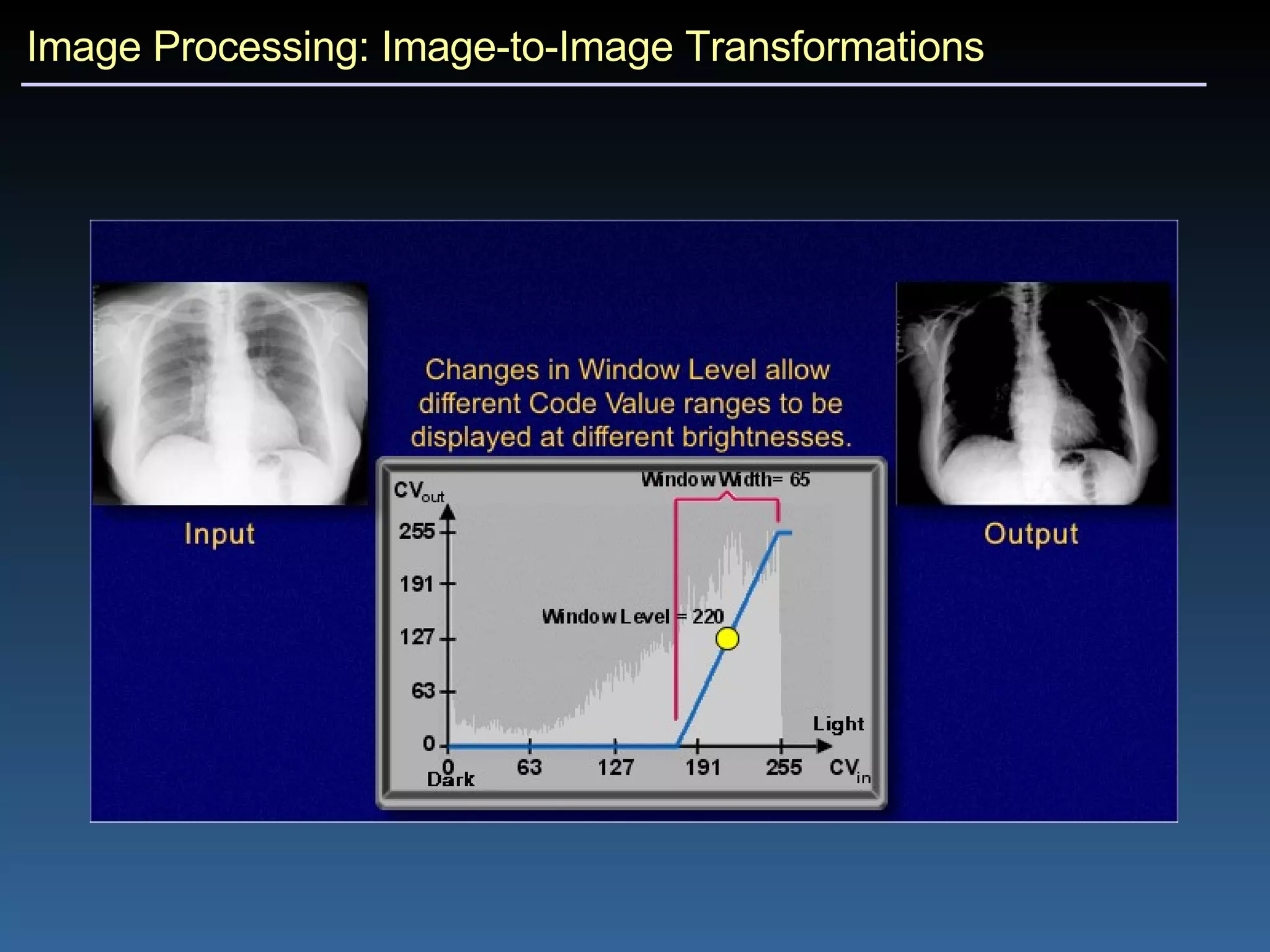
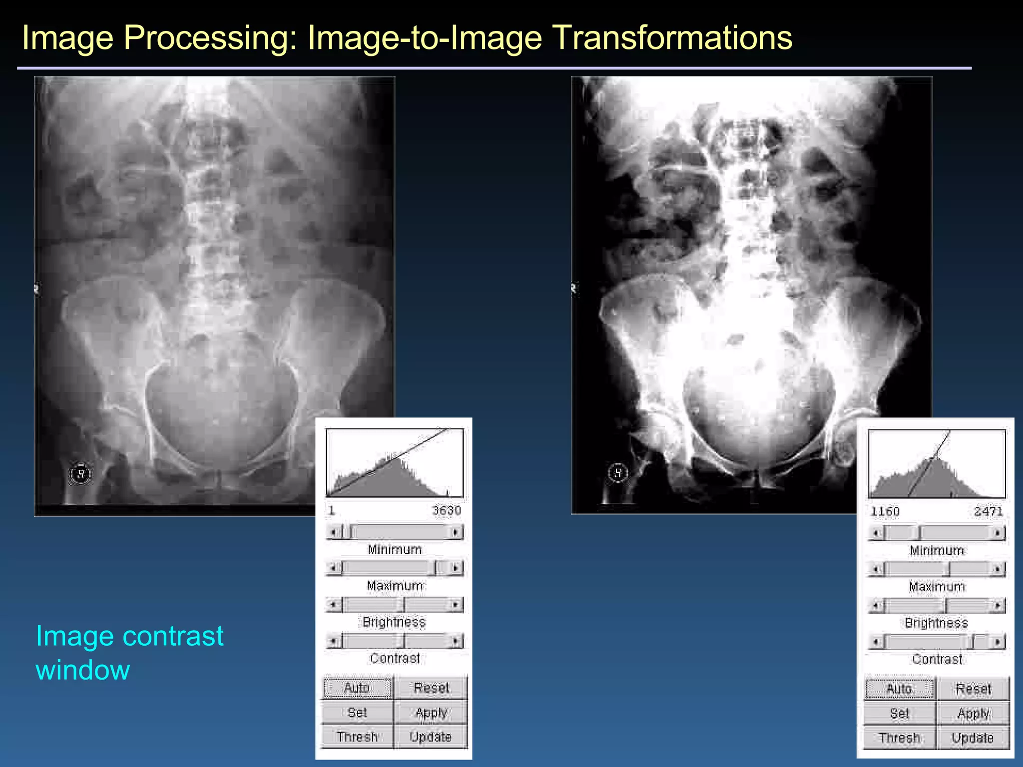
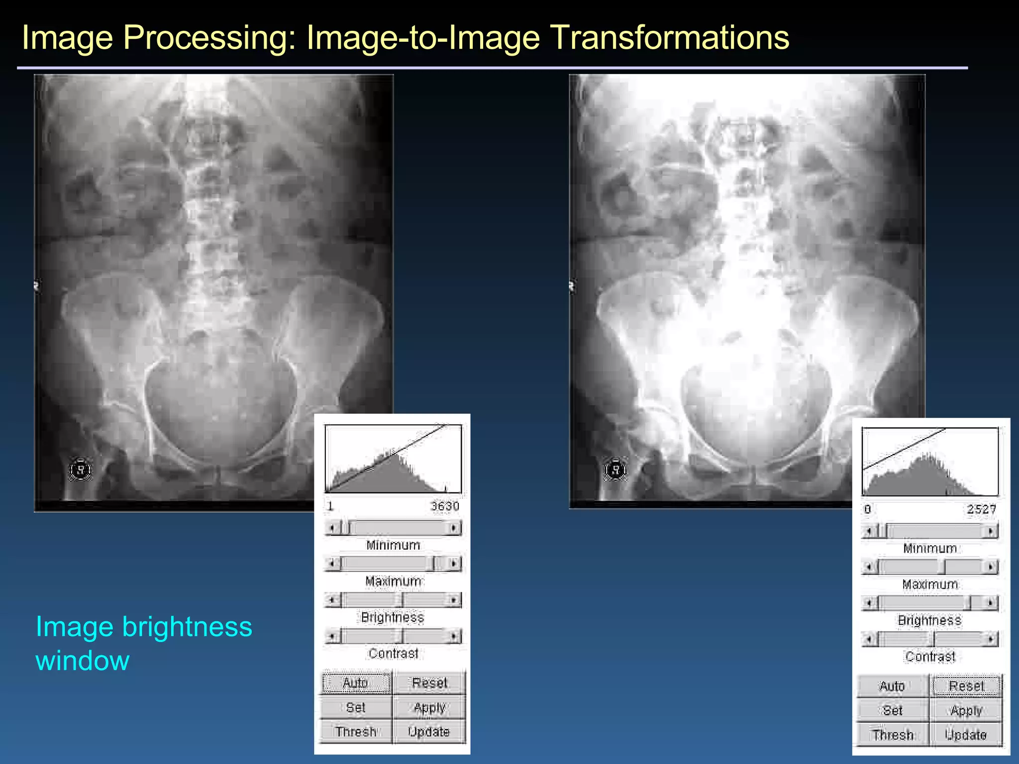
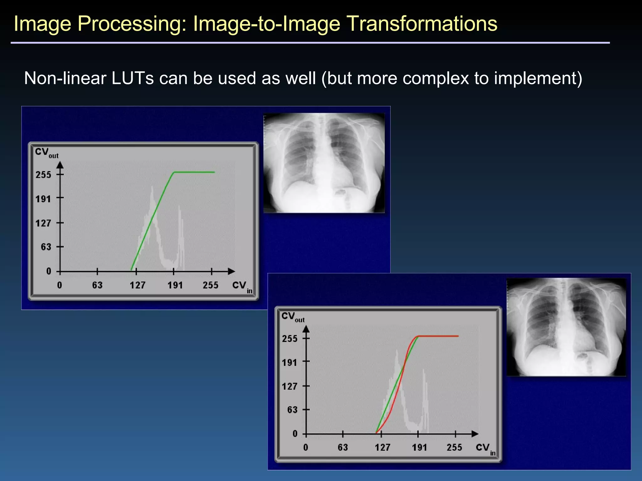

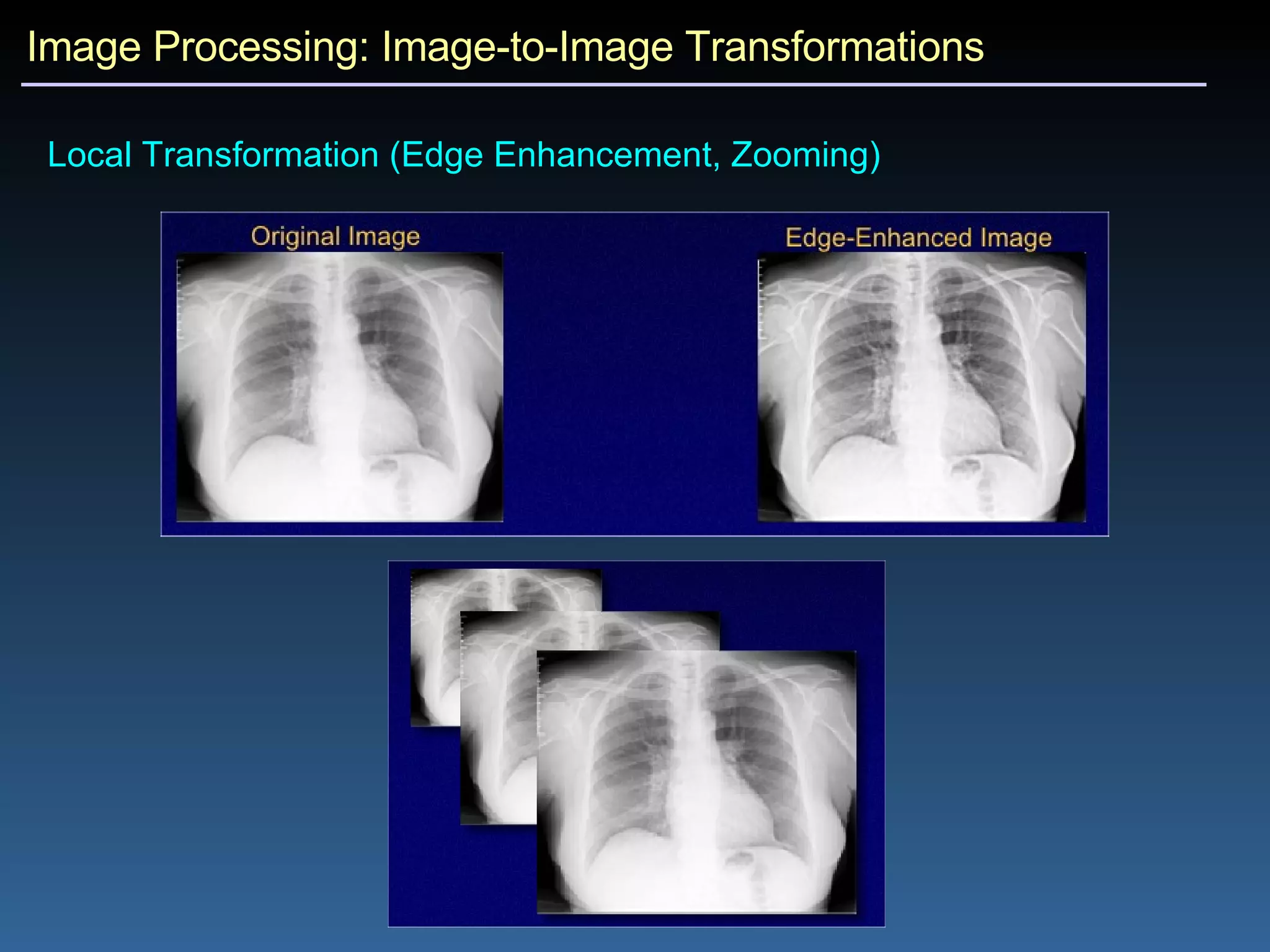
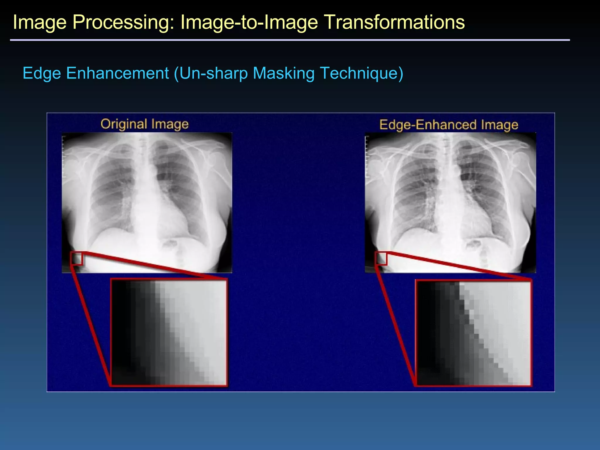

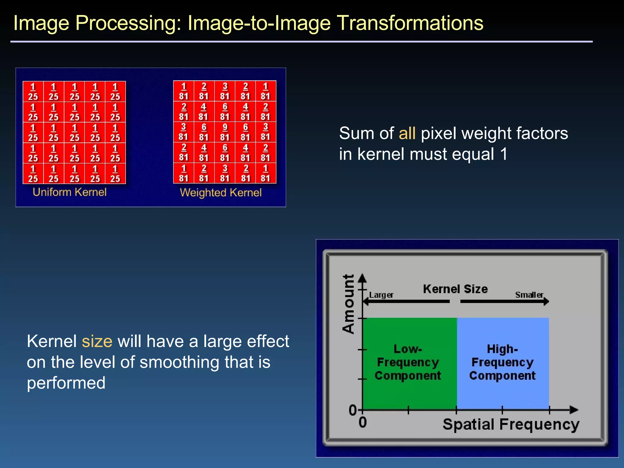
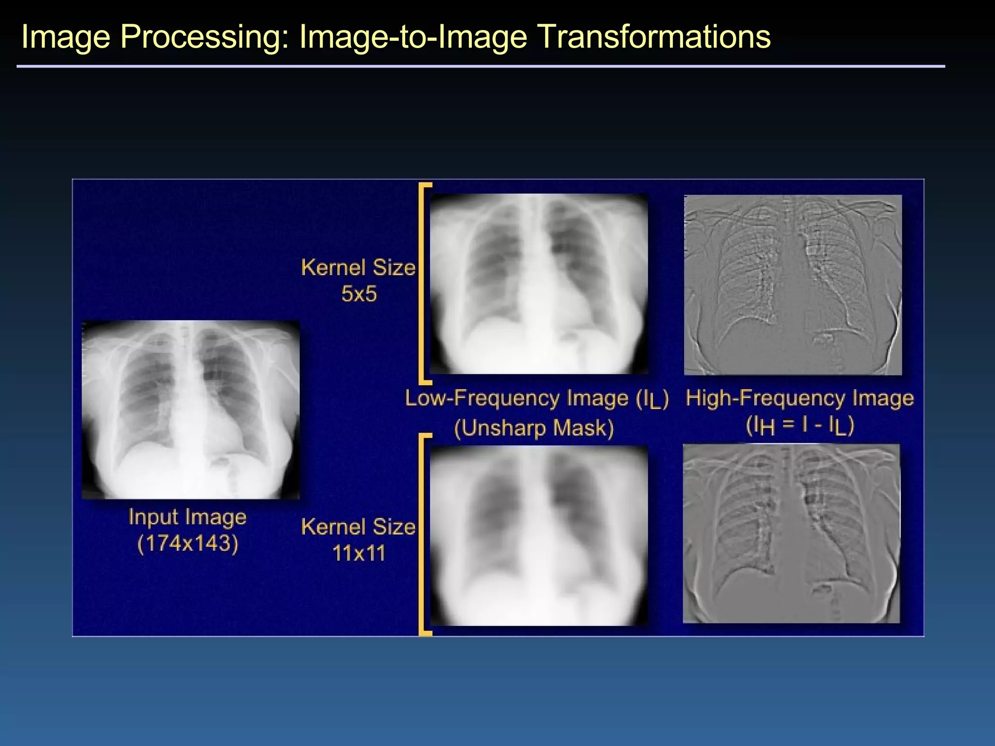
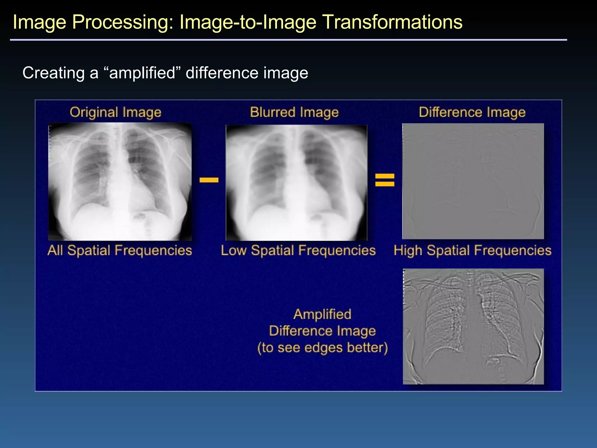
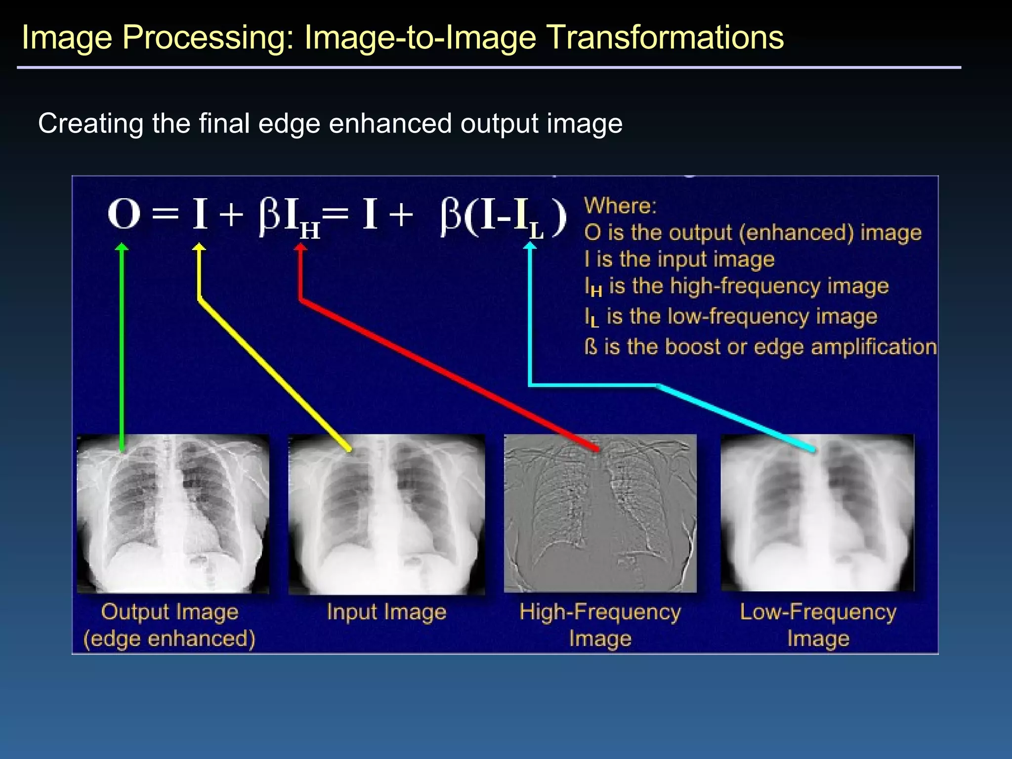
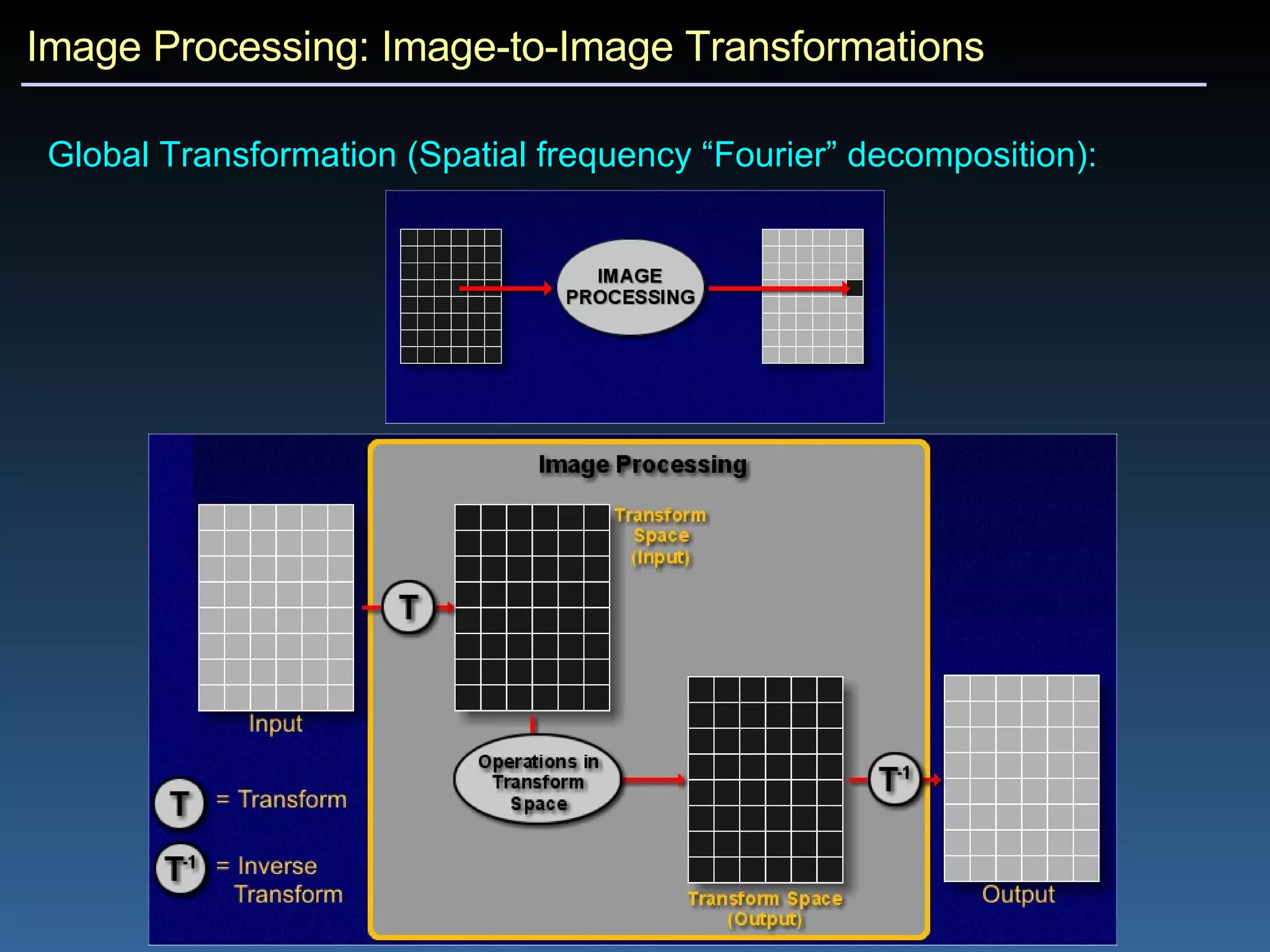
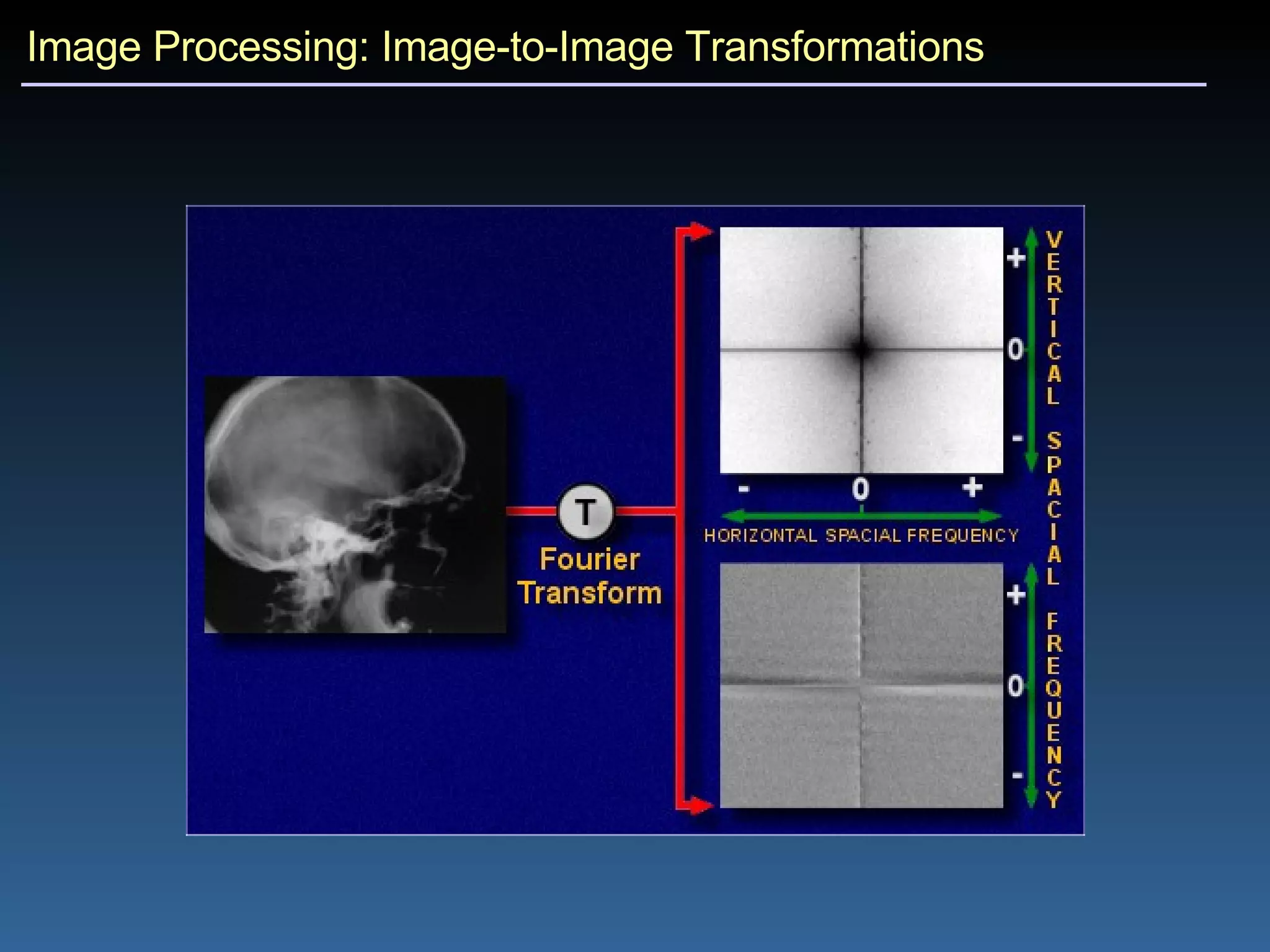
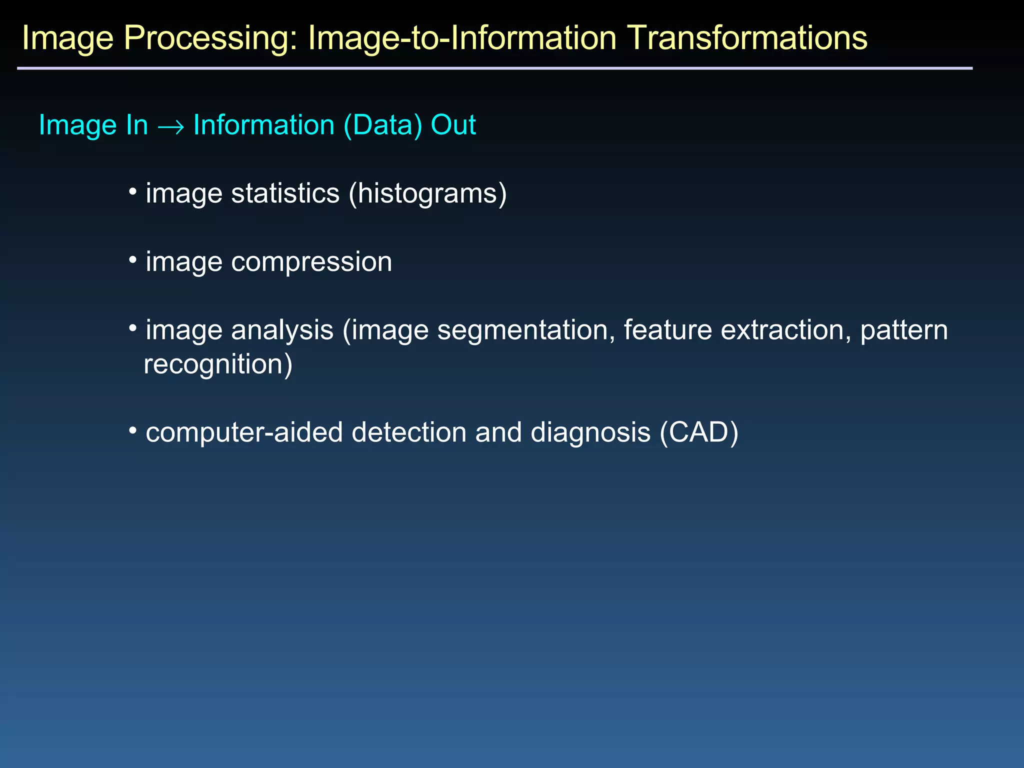
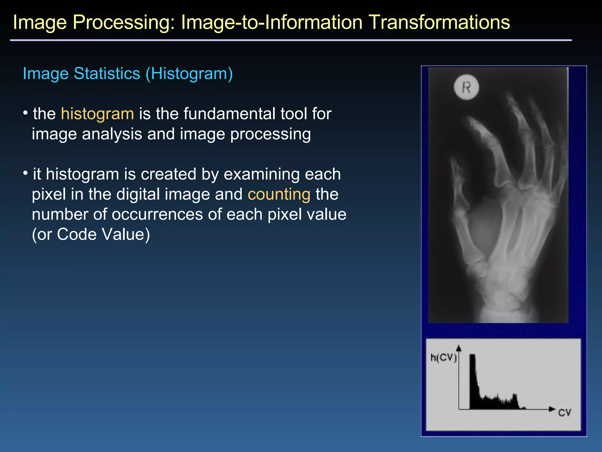
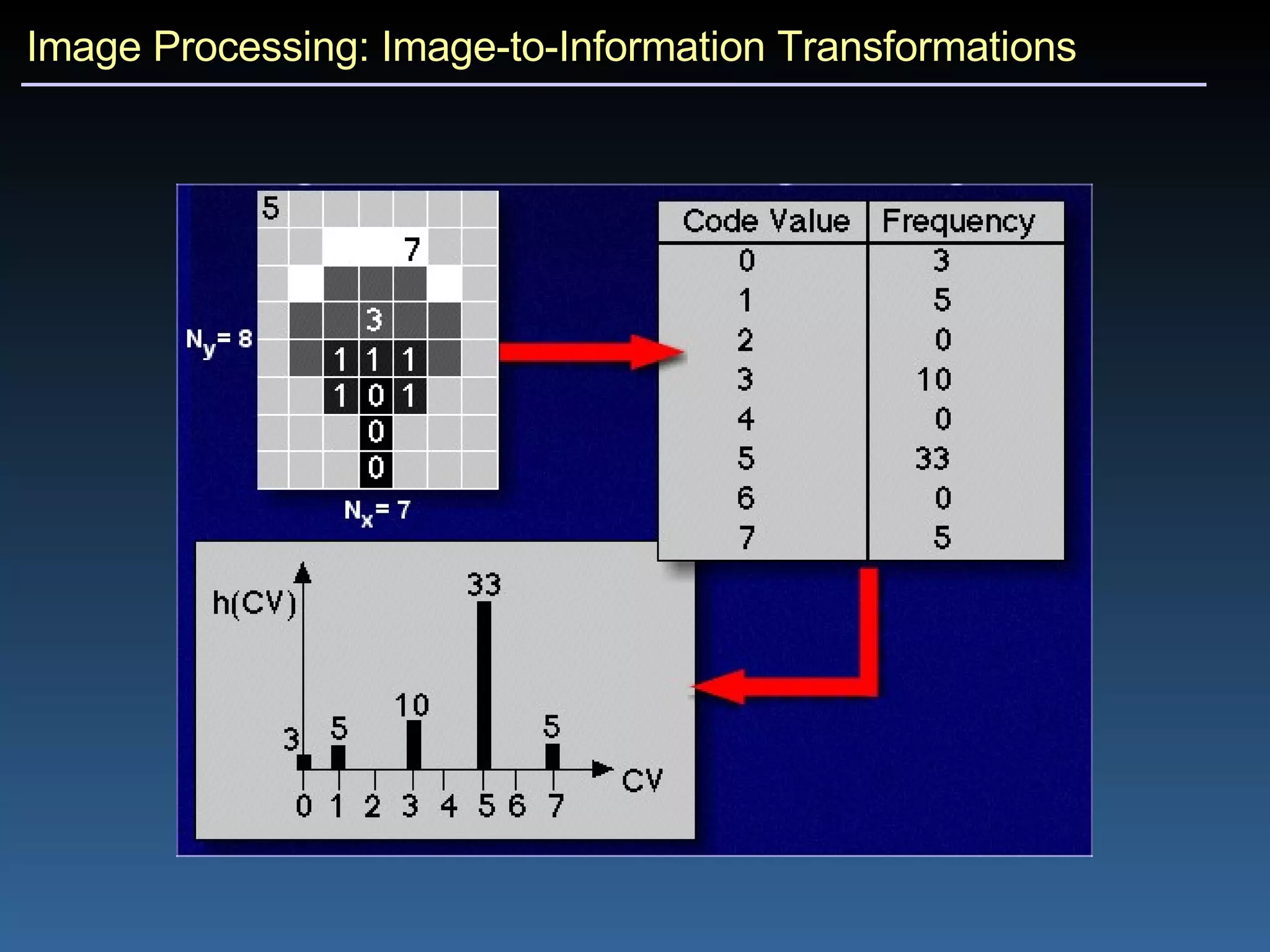
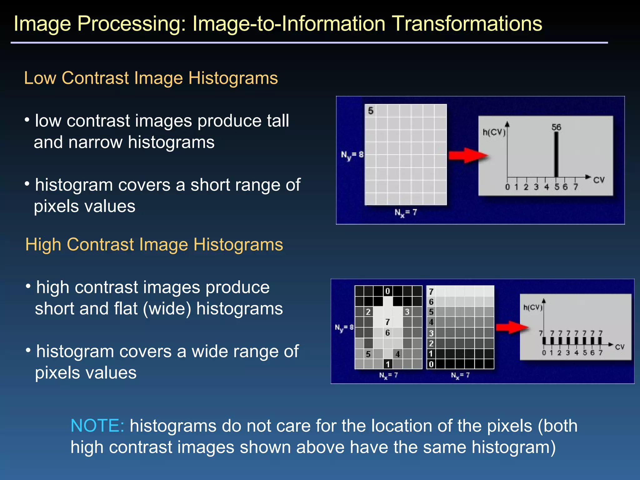
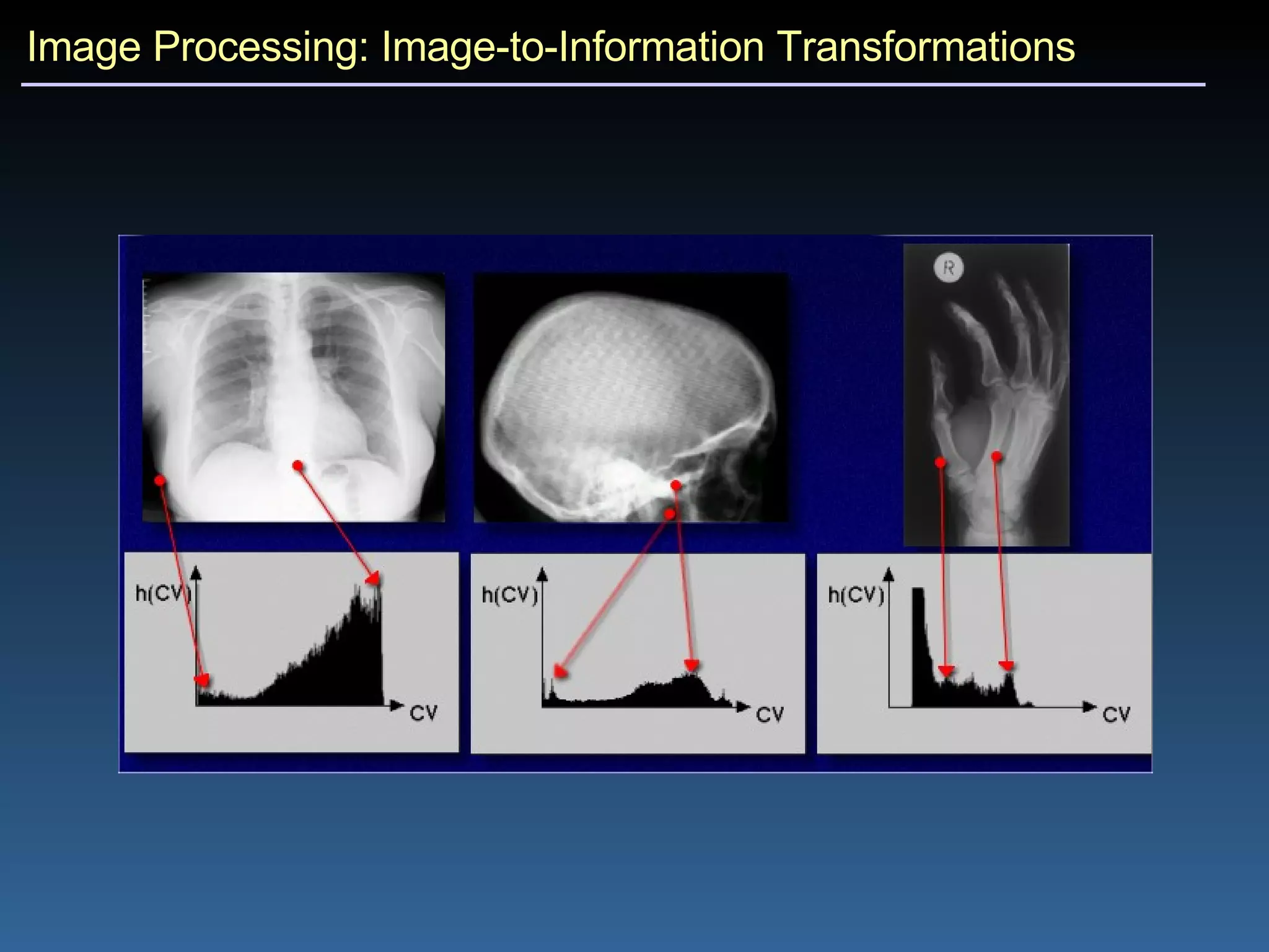

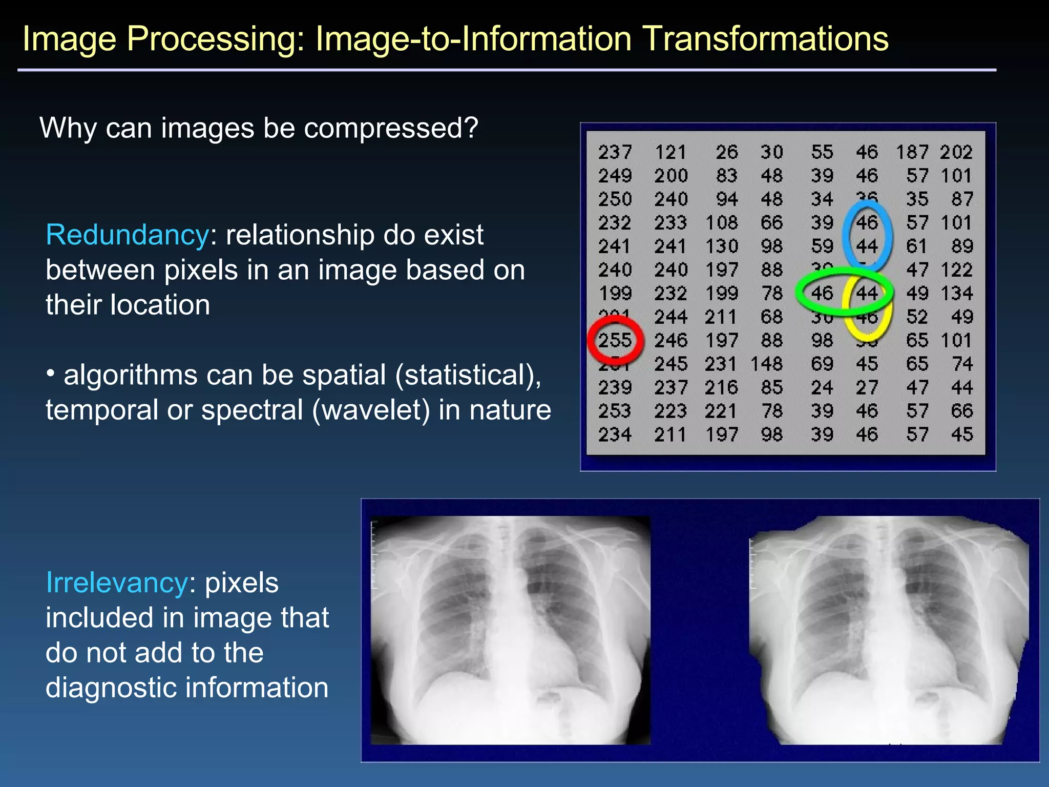
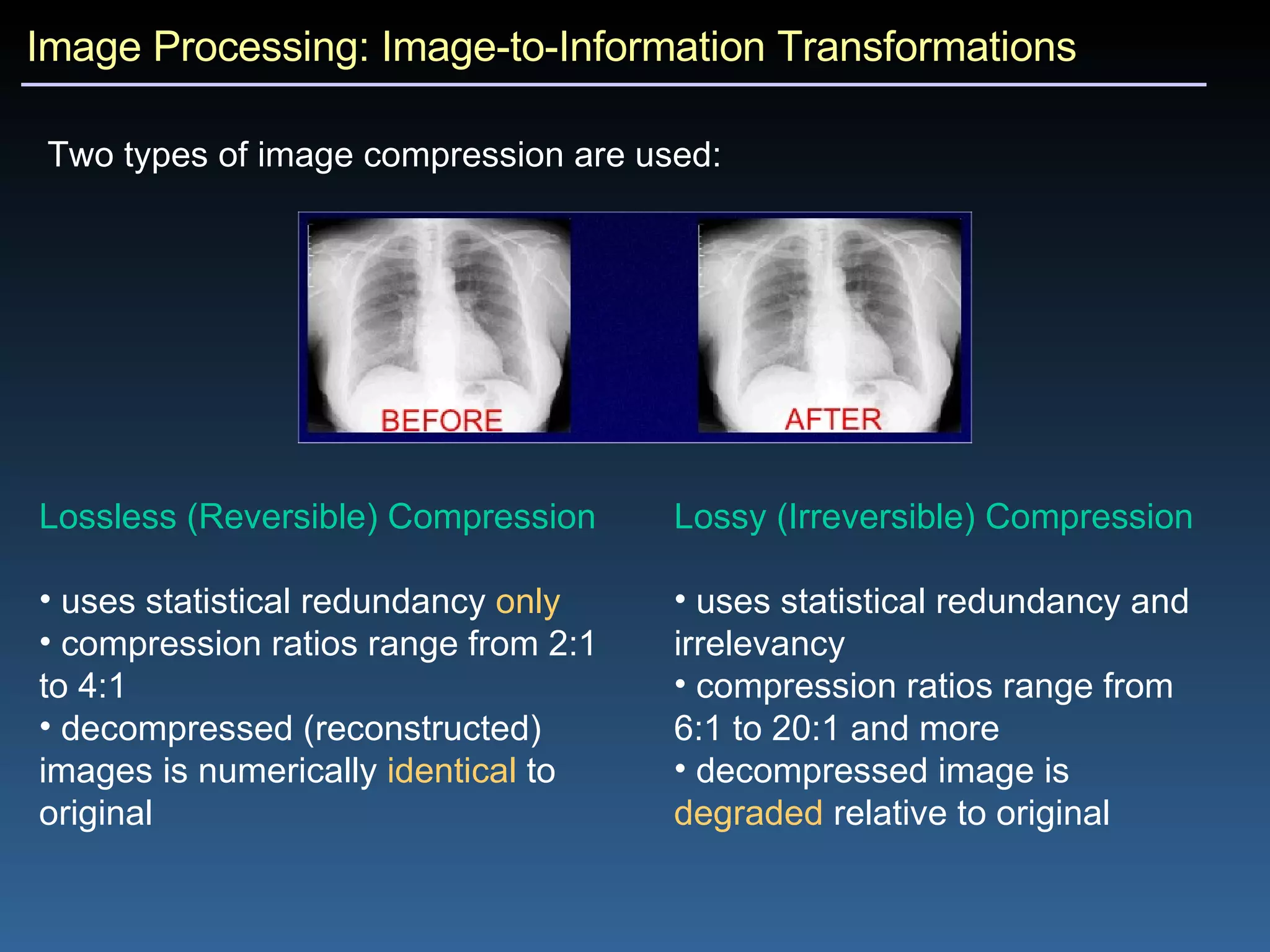
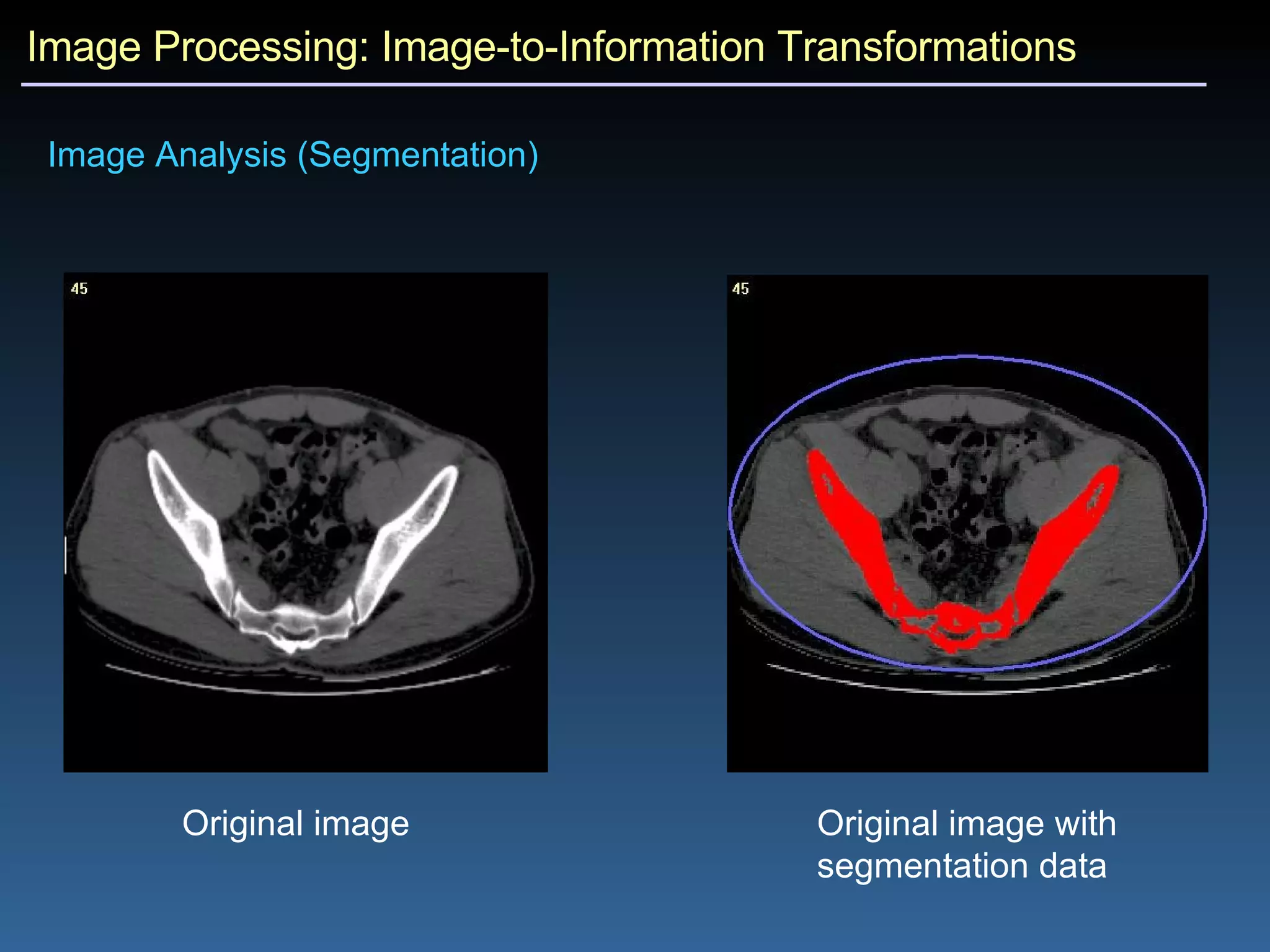
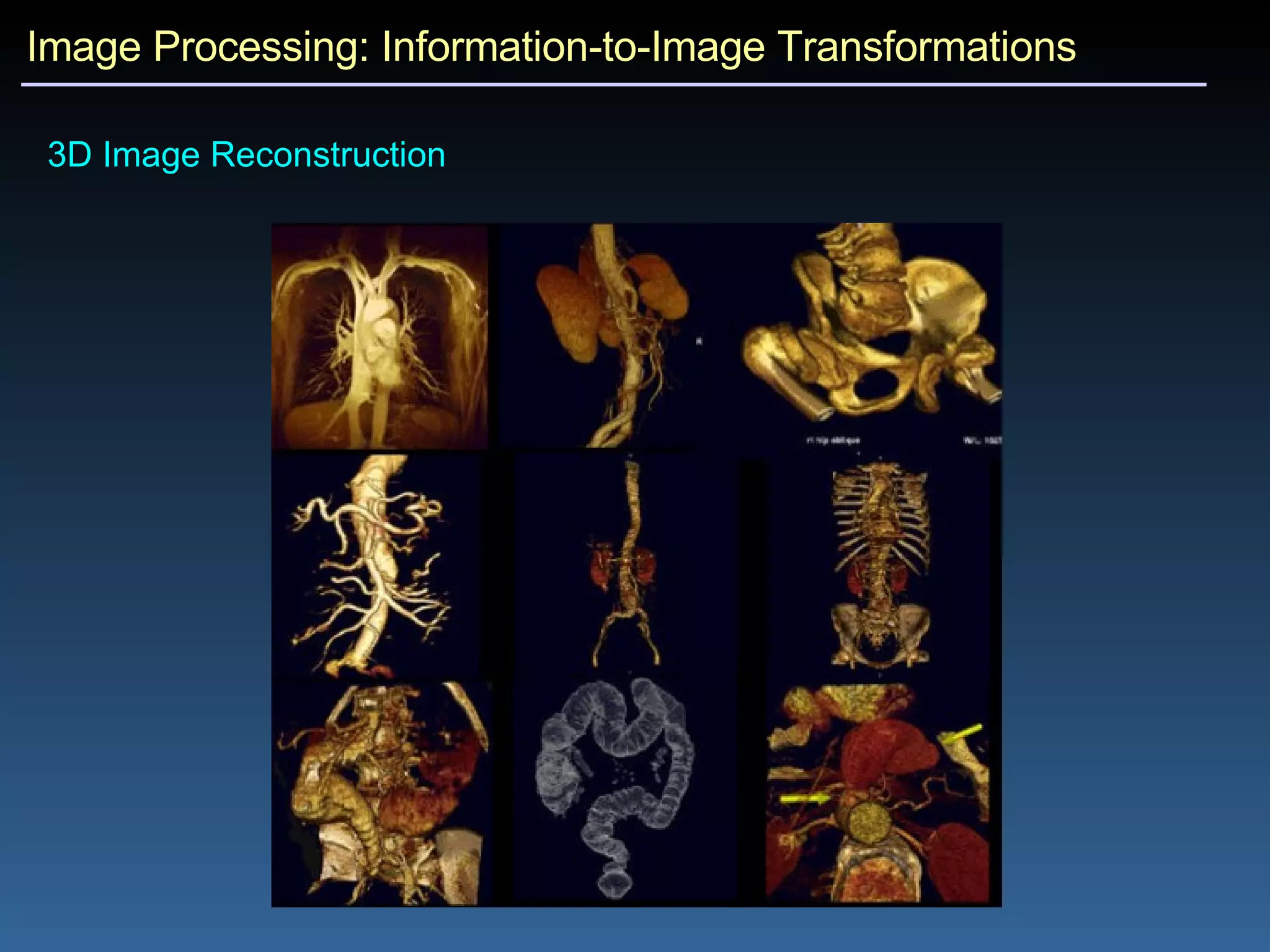
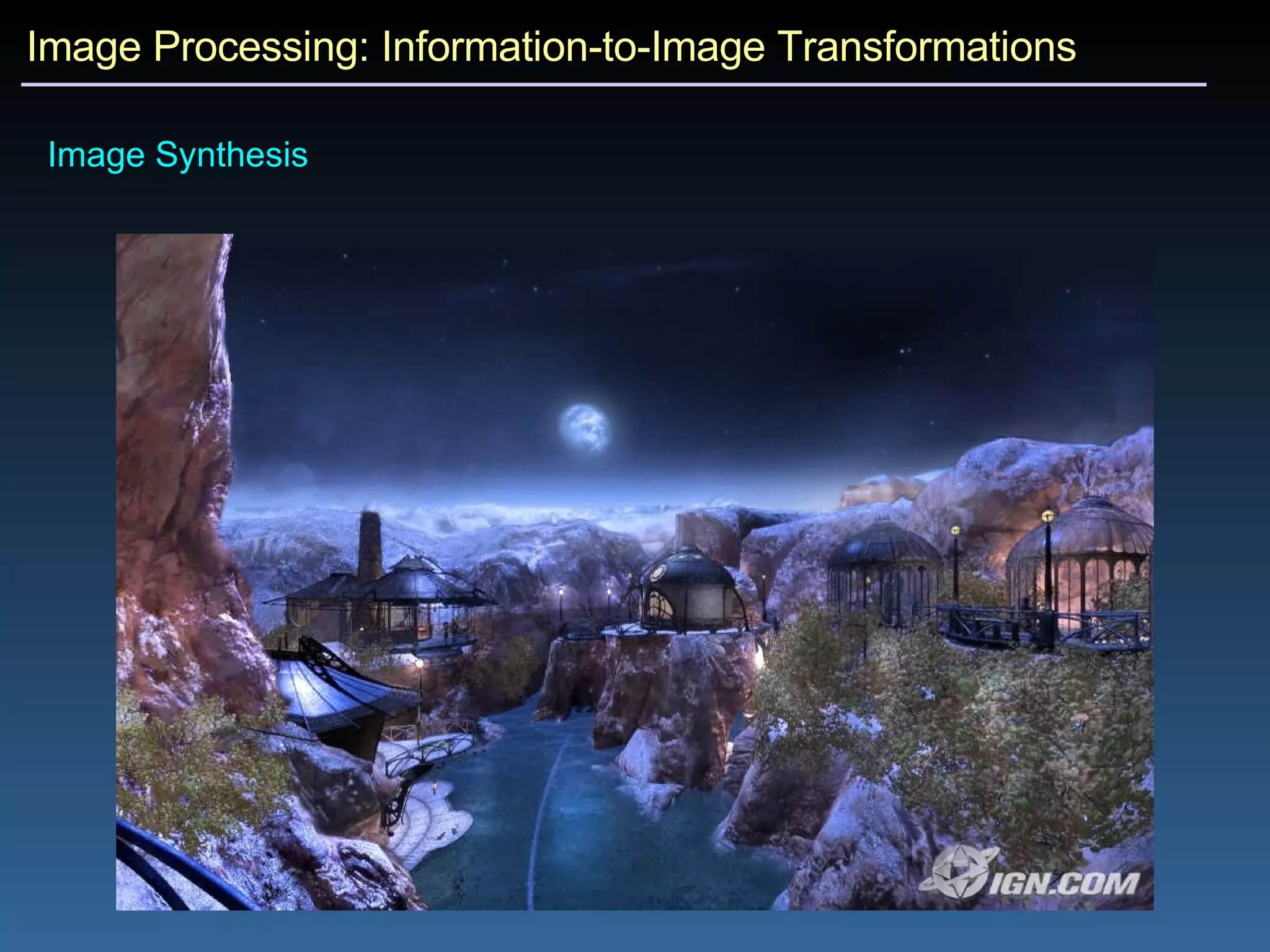
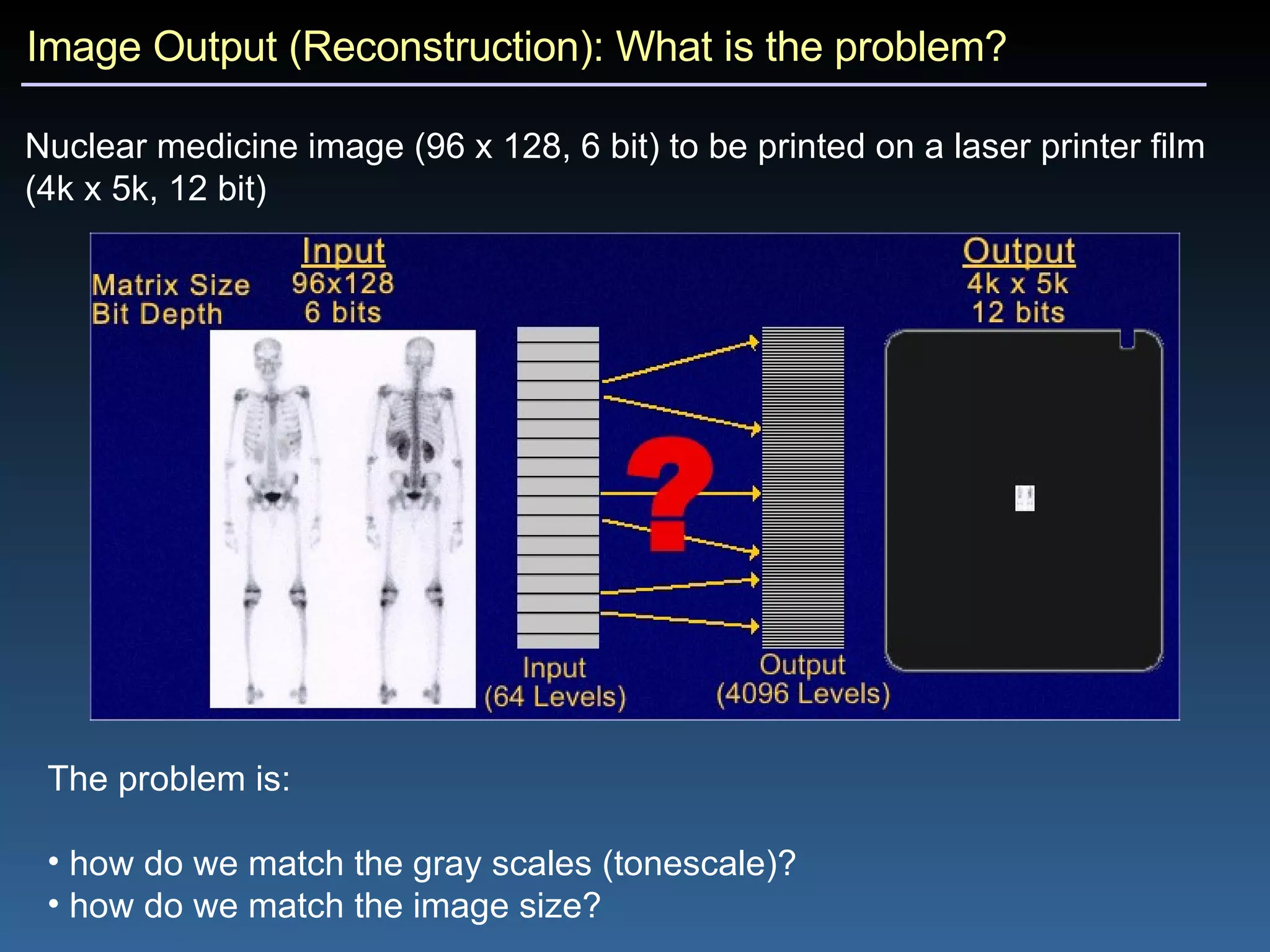


This document summarizes key concepts in digital image processing, including: 1) Image processing transforms digital images for viewing or analysis and includes image-to-image, image-to-information, and information-to-image transformations. 2) Image-to-image transformations like adjustments to tonescale, contrast, and geometry are used to enhance or alter digital images for output or diagnosis. 3) Image-to-information transformations extract data from images through techniques like histograms, compression, and segmentation for analysis. 4) Information-to-image transformations are needed to reconstruct images for output through techniques like decompression and scaling.


