Downloaded 16 times
![Operational Semantics -- Evaluation
t1 t1'
/* congruence rule 1 */
t1 t2 t1' t2
t2 t2'
/* congruence rule 2 */
v1 t2 v1 t2'
(λx.t) v [x ↦ v]t /* computation rule */](https://image.slidesharecdn.com/introductiontothelambdacalculus-170119234004/85/Introduction-to-the-lambda-calculus-3-320.jpg)

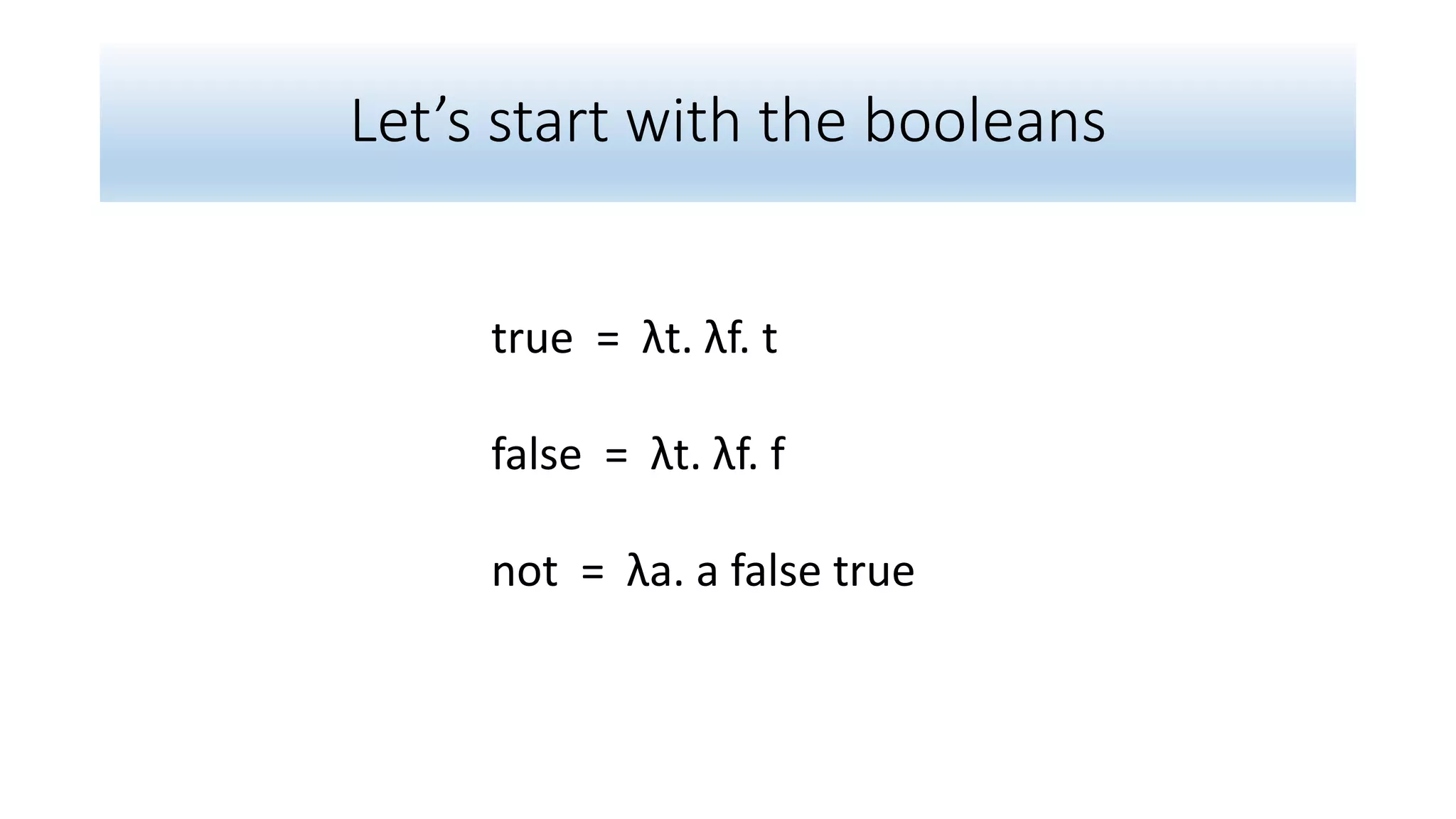
![Applying not
(λa. a false true) true
(λa. a false true) (λt. λf. t)
(λt. λf. t) false true
false
(λx.t) v [x ↦ v]t
(from operational semantic rules)](https://image.slidesharecdn.com/introductiontothelambdacalculus-170119234004/85/Introduction-to-the-lambda-calculus-8-320.jpg)


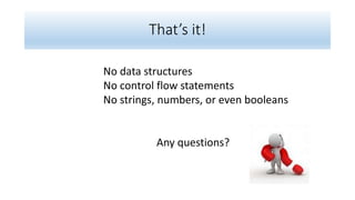
![Operational Semantics -- Evaluation
t1 t1'
/* congruence rule 1 */
t1 t2 t1' t2
t2 t2'
/* congruence rule 2 */
v1 t2 v1 t2'
(λx.t) v [x ↦ v]t /* computation rule */](https://image.slidesharecdn.com/introductiontothelambdacalculus-170119234004/75/Introduction-to-the-lambda-calculus-3-2048.jpg)

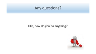
![Applying not
(λa. a false true) true
(λa. a false true) (λt. λf. t)
(λt. λf. t) false true
false
(λx.t) v [x ↦ v]t
(from operational semantic rules)](https://image.slidesharecdn.com/introductiontothelambdacalculus-170119234004/75/Introduction-to-the-lambda-calculus-8-2048.jpg)

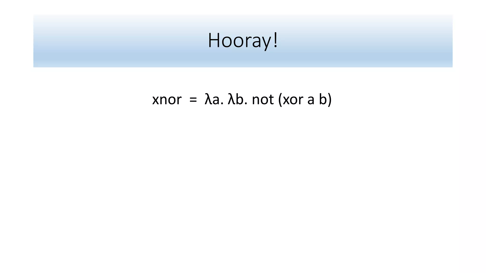
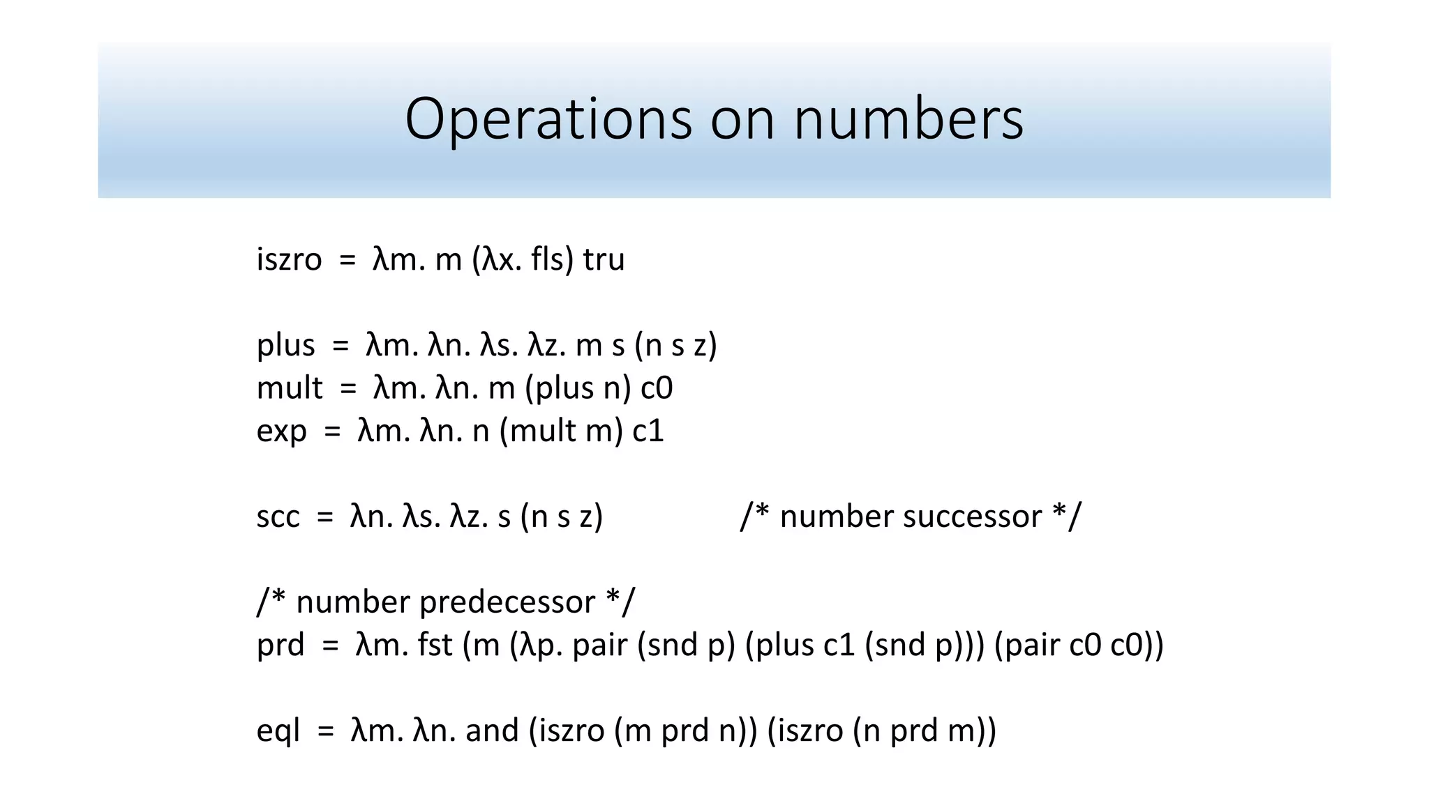
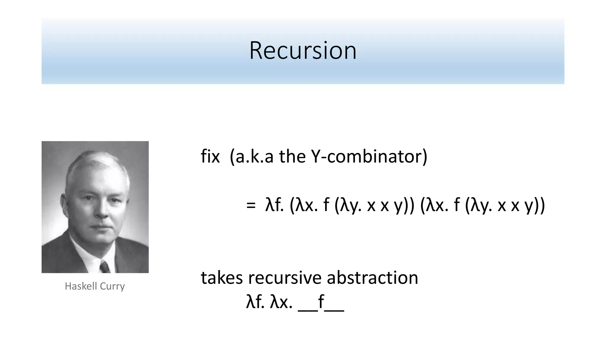
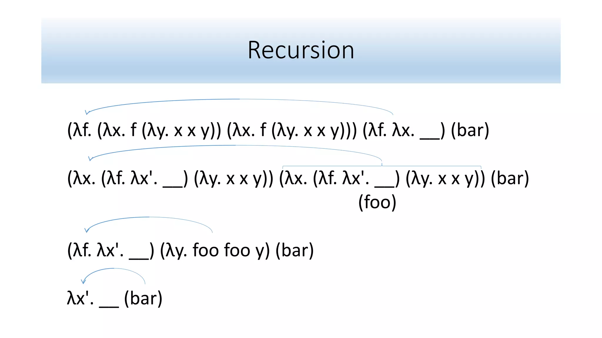
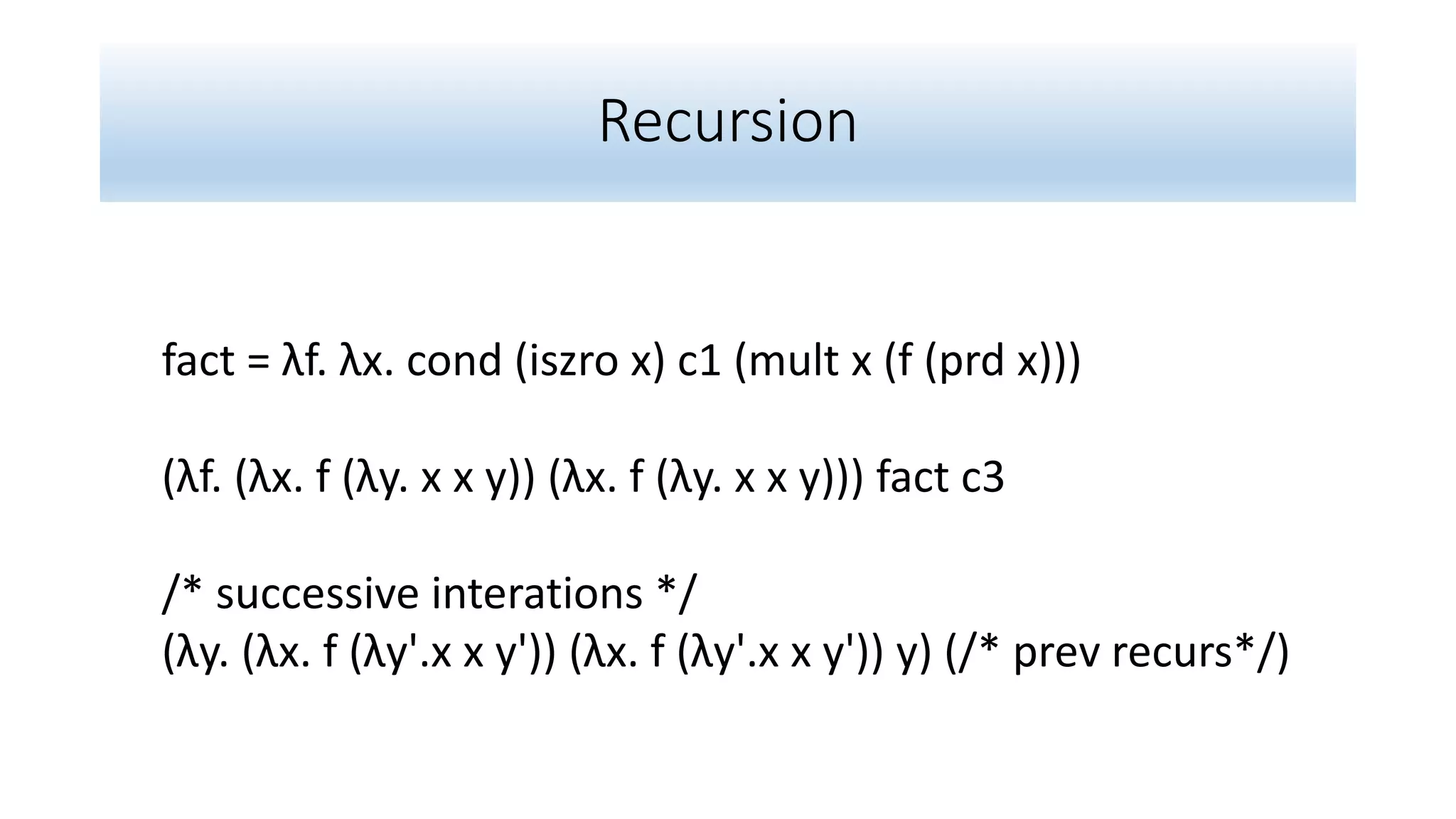

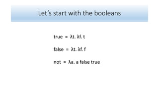
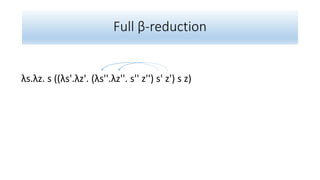
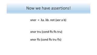
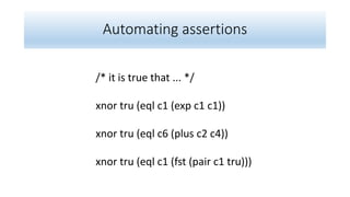
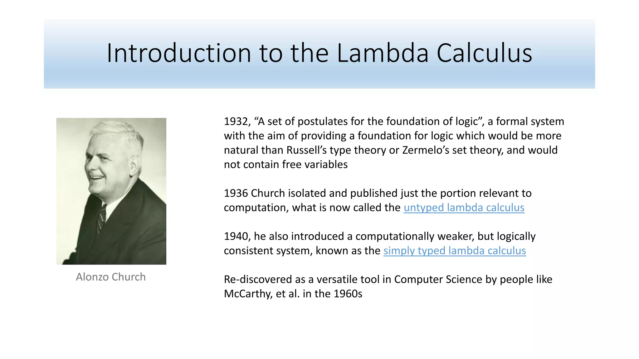
This document introduces the lambda calculus through its history and key concepts. It describes Alonzo Church's development of the untyped and simply typed lambda calculus in the 1930s and 1940s as a foundation for logic and computation. It then explains the basic syntax and evaluation rules of the lambda calculus, how to represent data like booleans and numbers, and how to define common operations and recursion without built-in types or control structures.


![[FLOLAC'14][scm] Functional Programming Using Haskell](https://cdn.slidesharecdn.com/ss_thumbnails/slides-140630030216-phpapp01-thumbnail.jpg?width=600ounds&width=560&fit=bounds)


