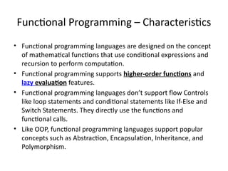
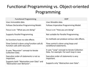
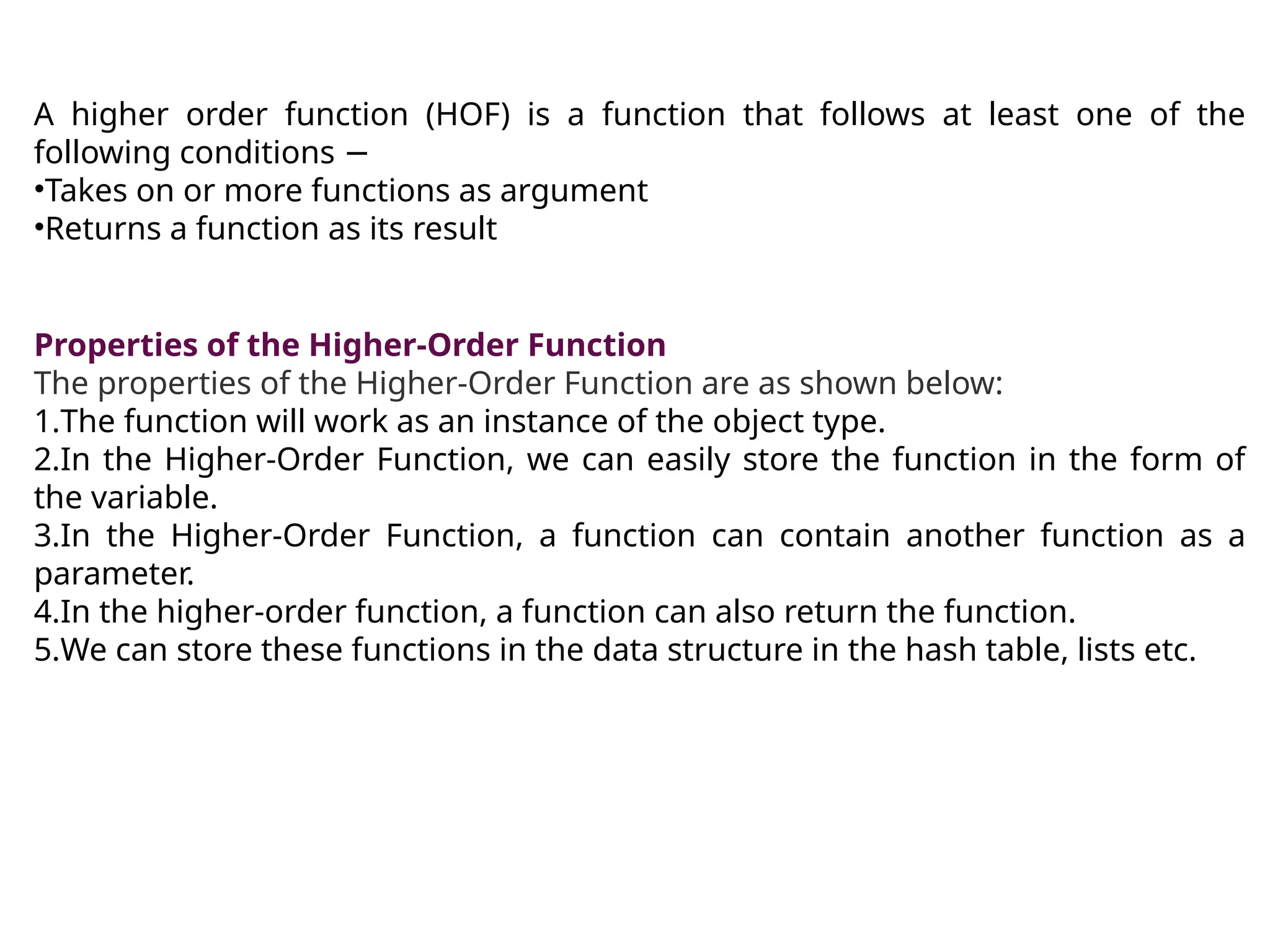
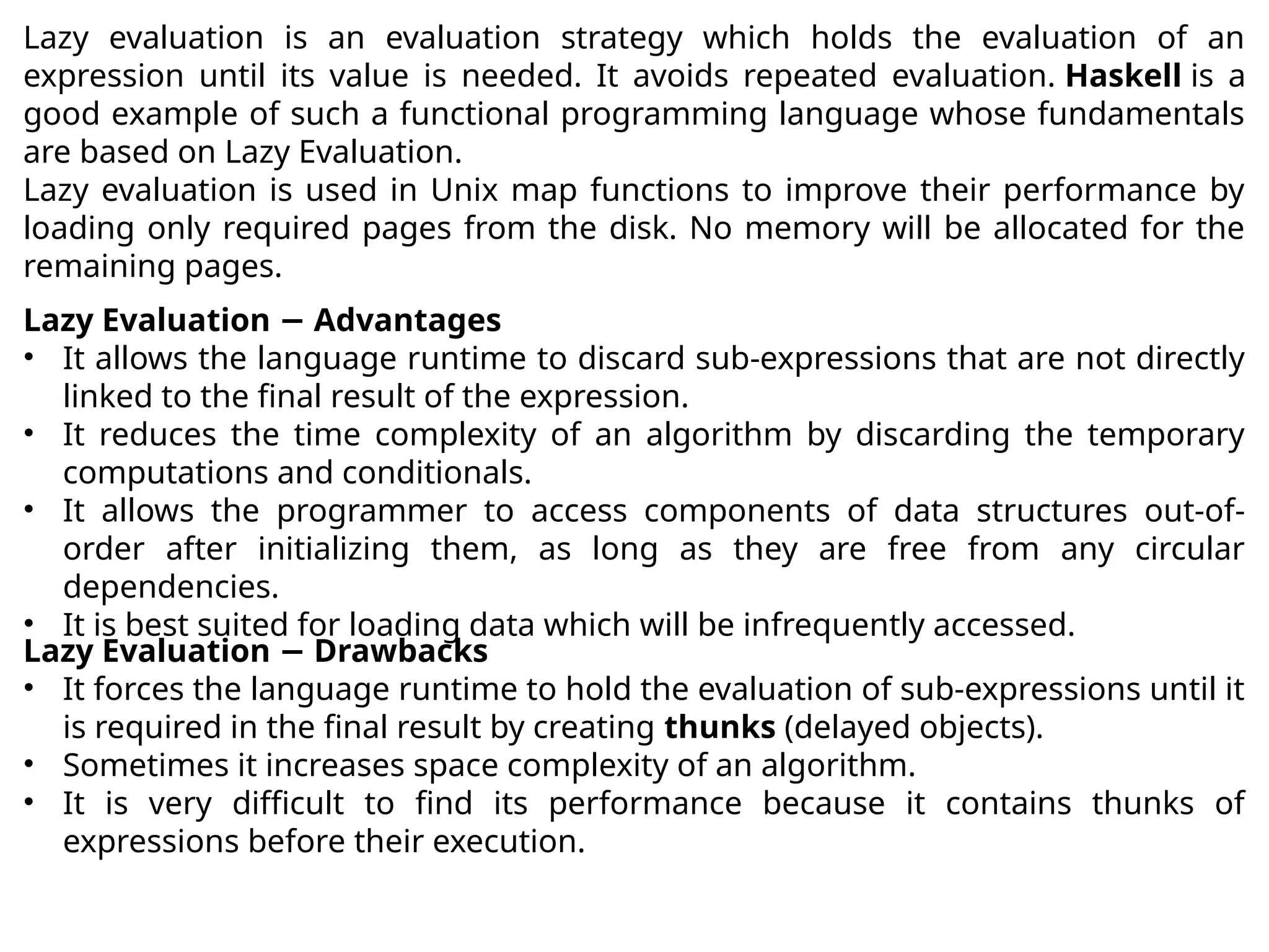
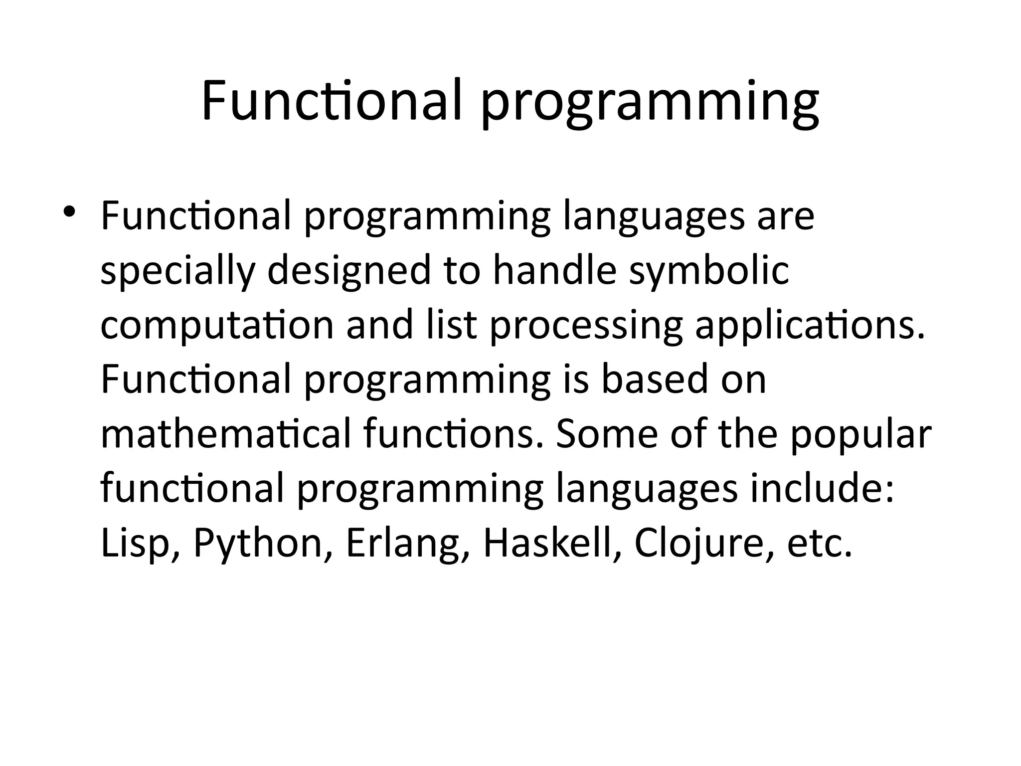
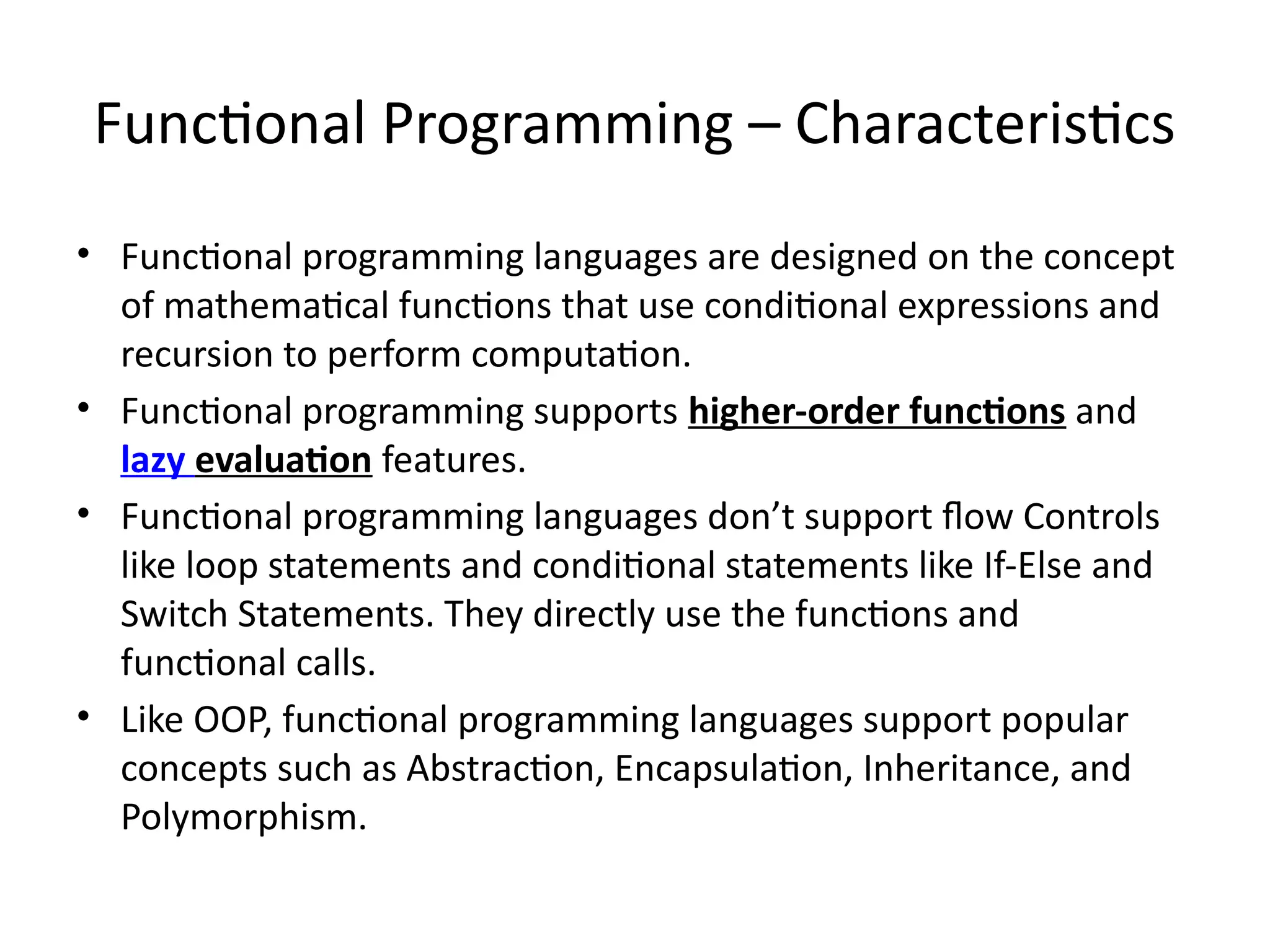
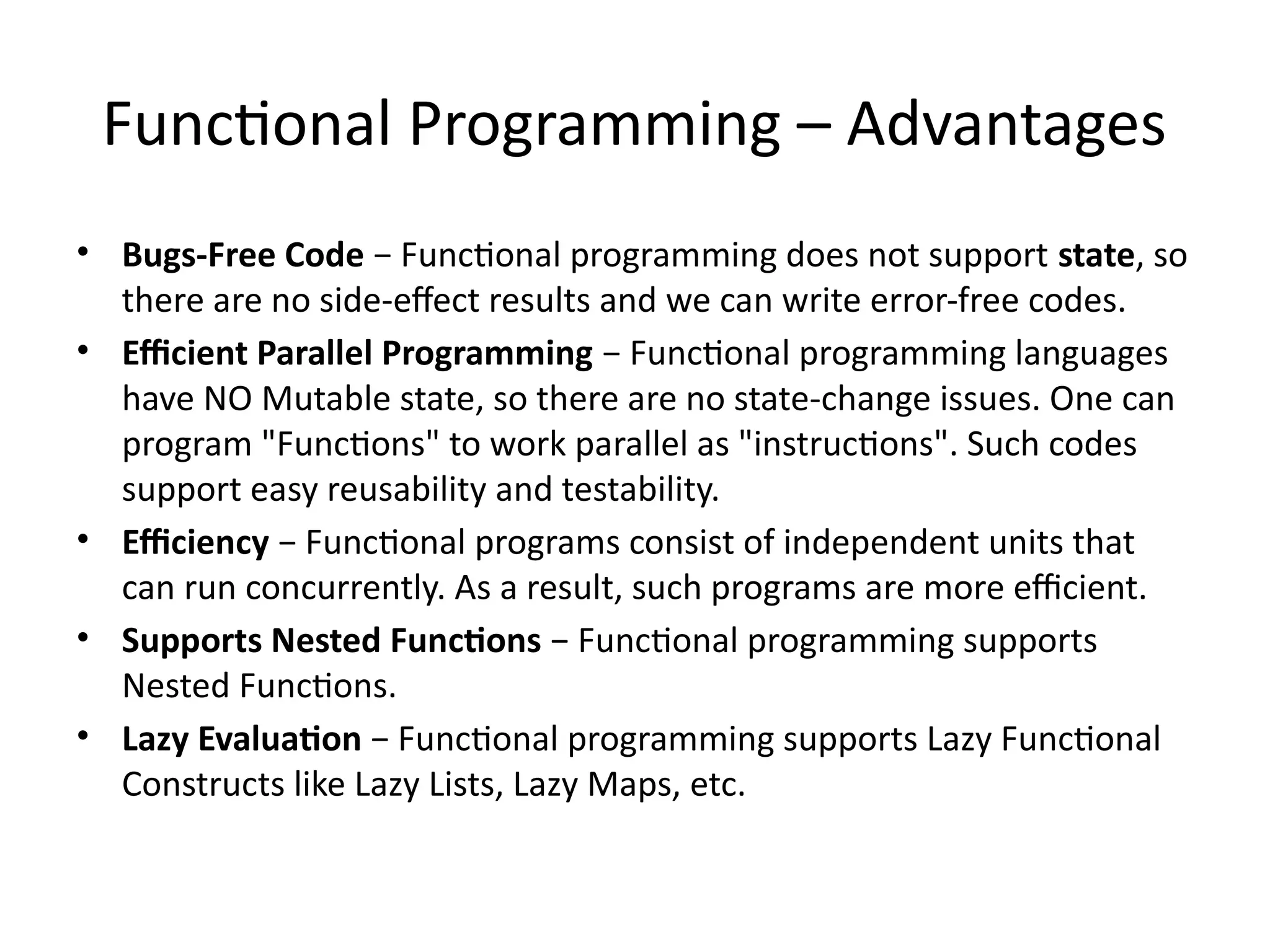
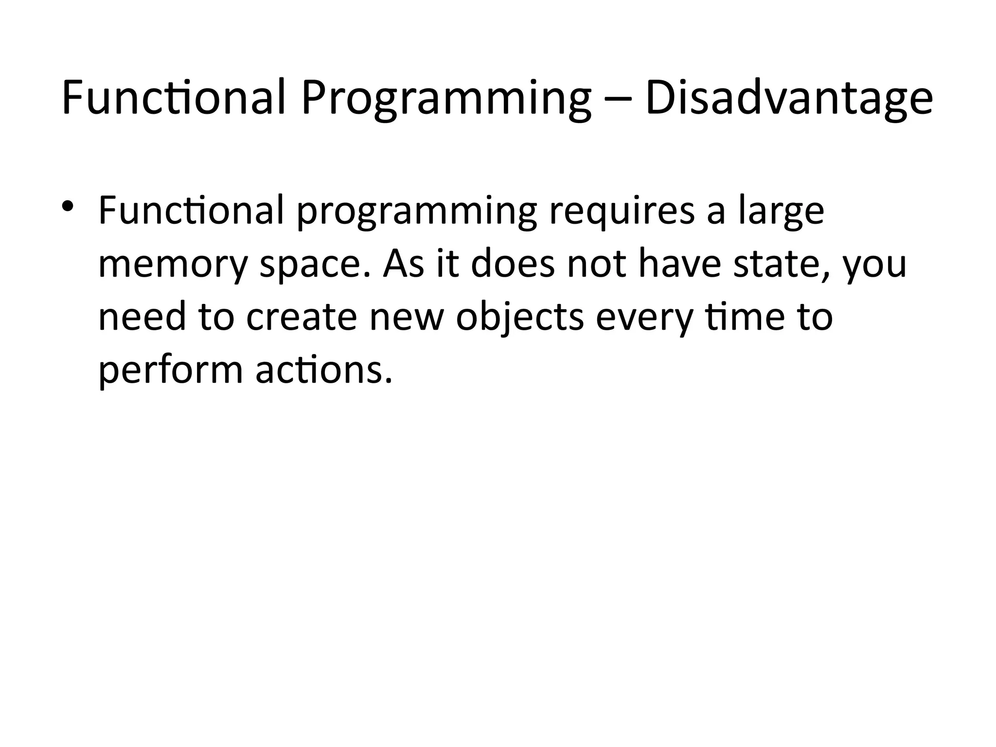
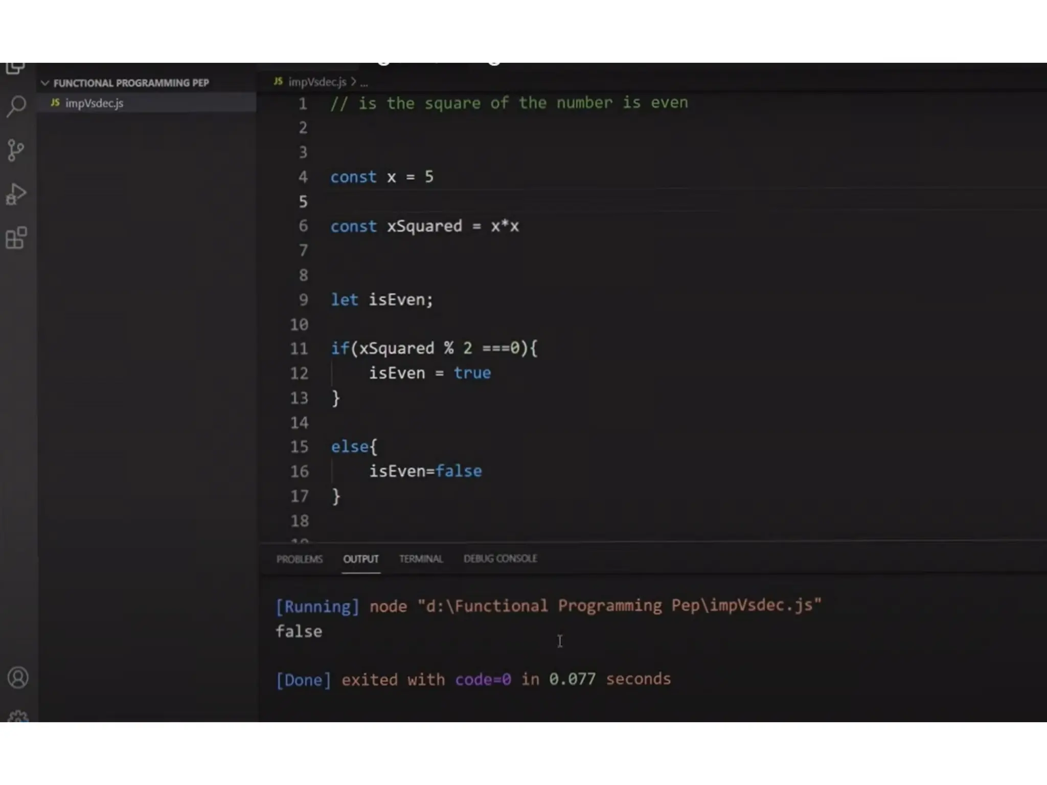
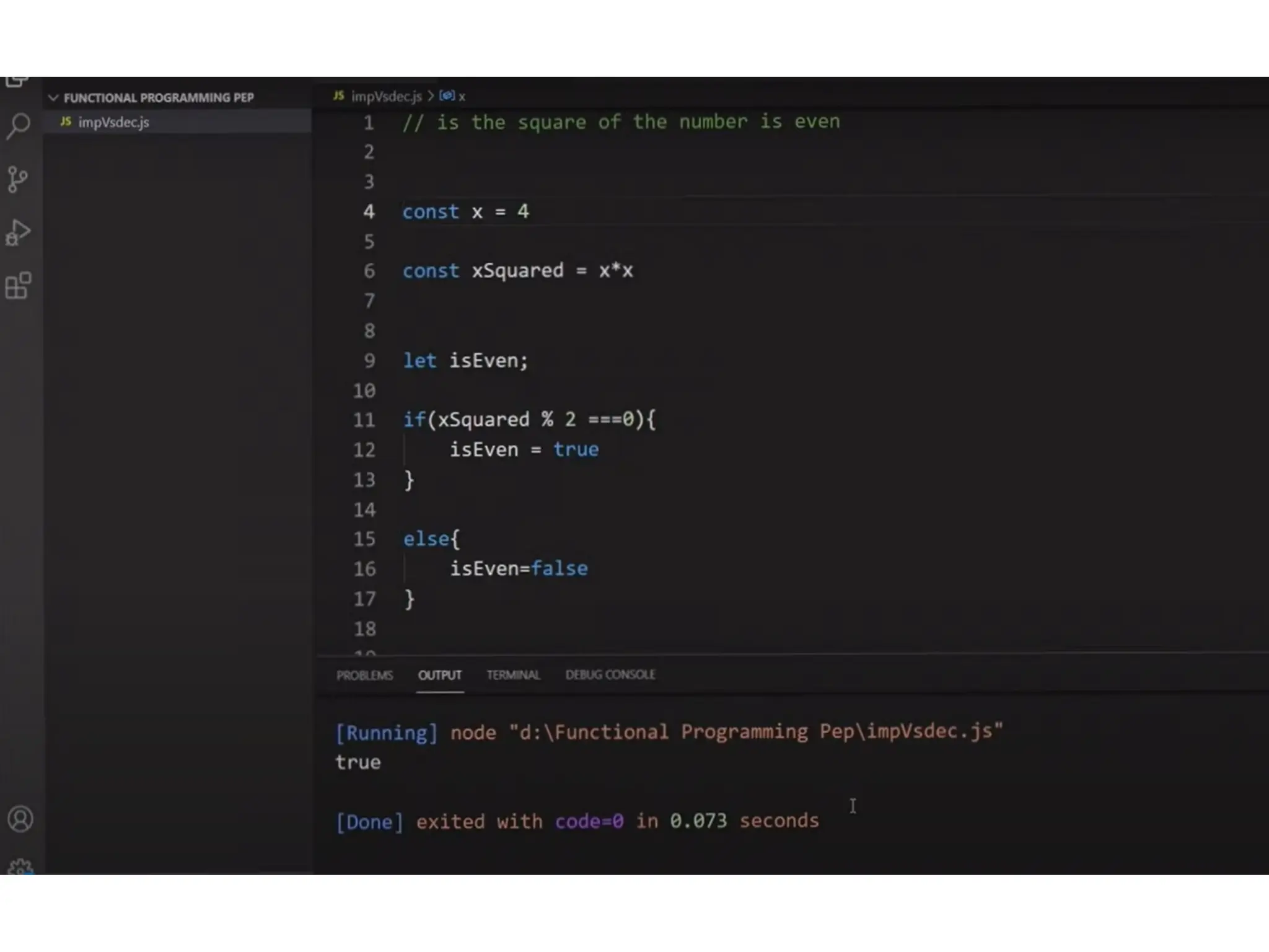
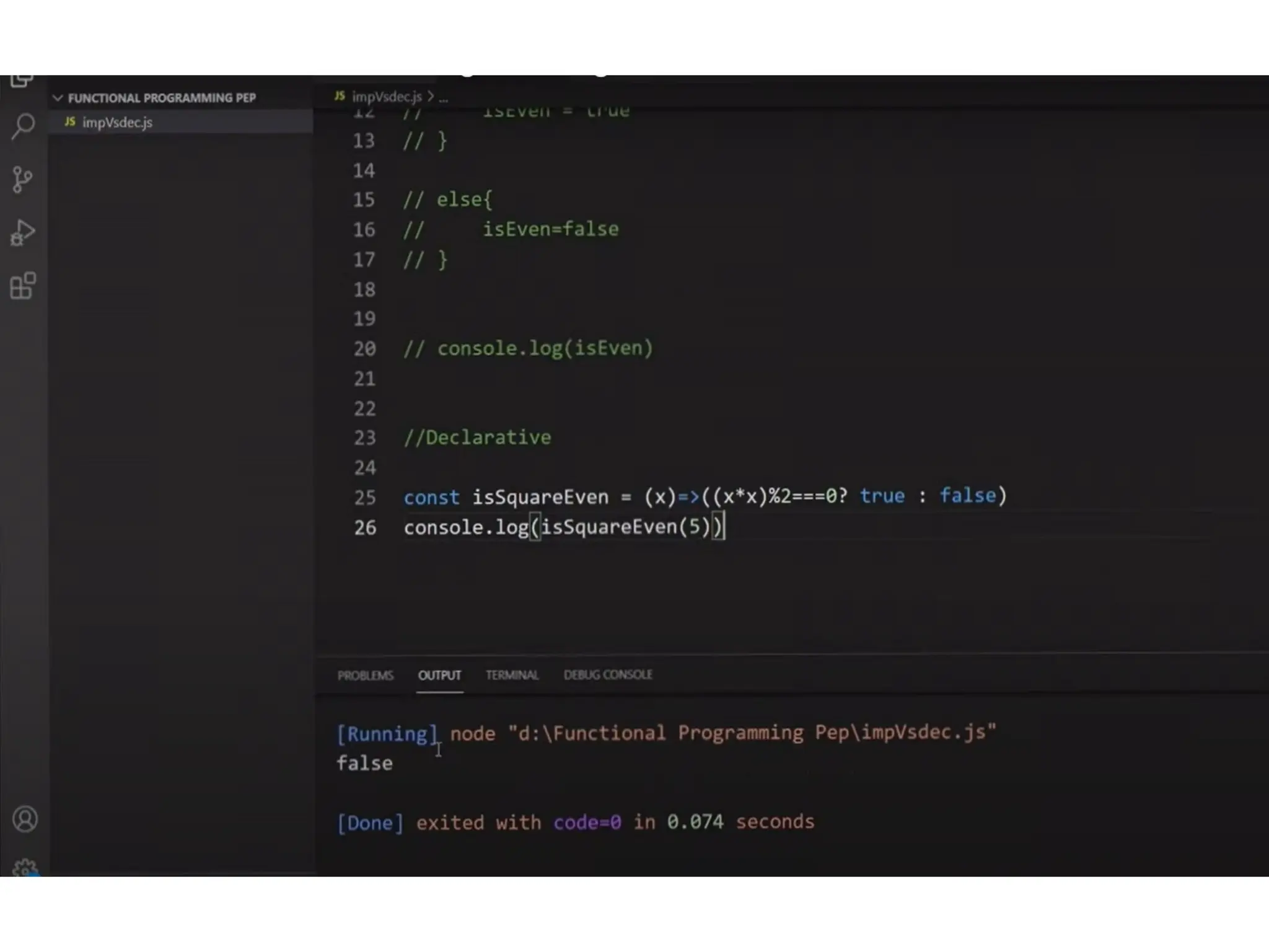
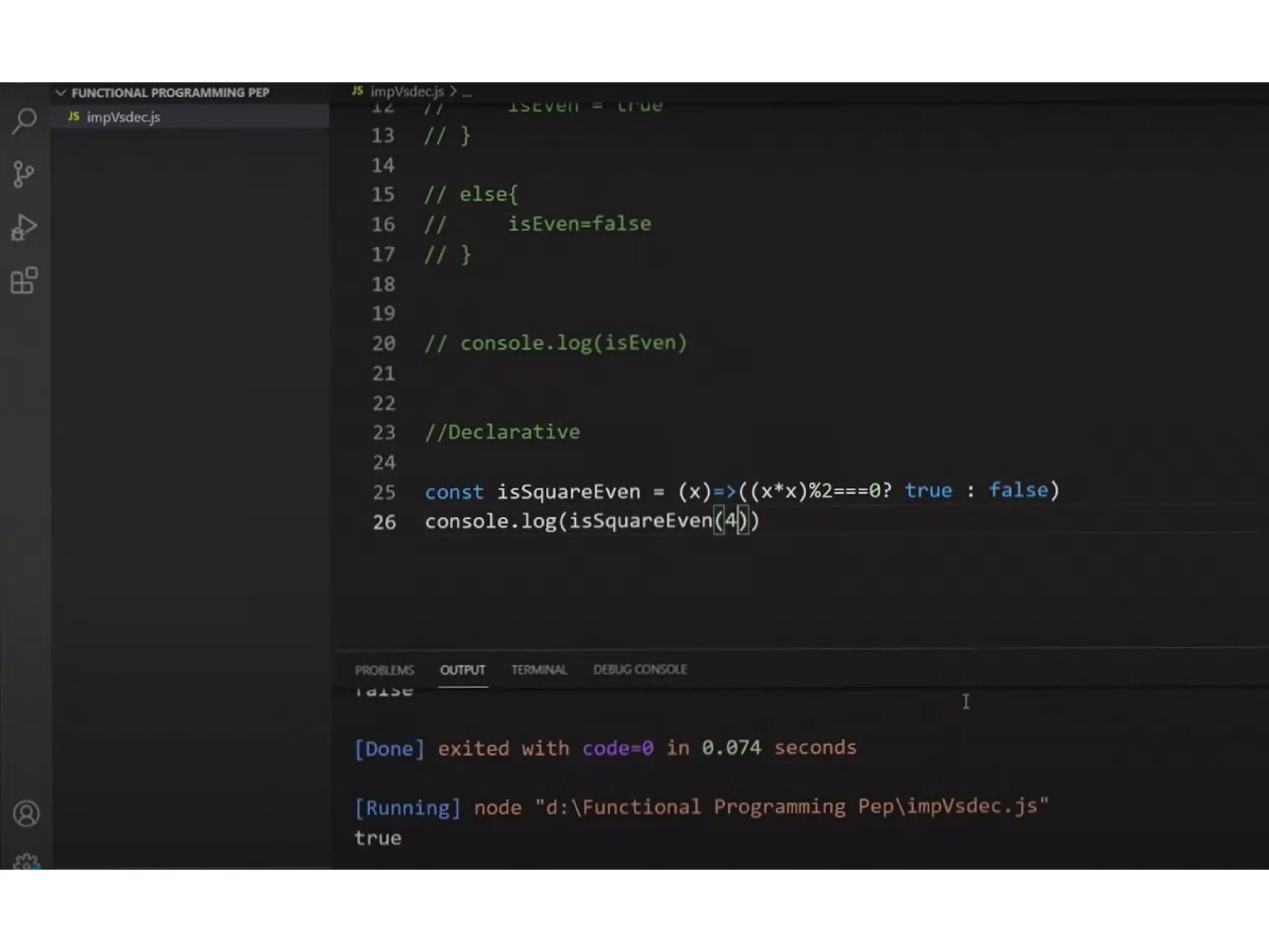
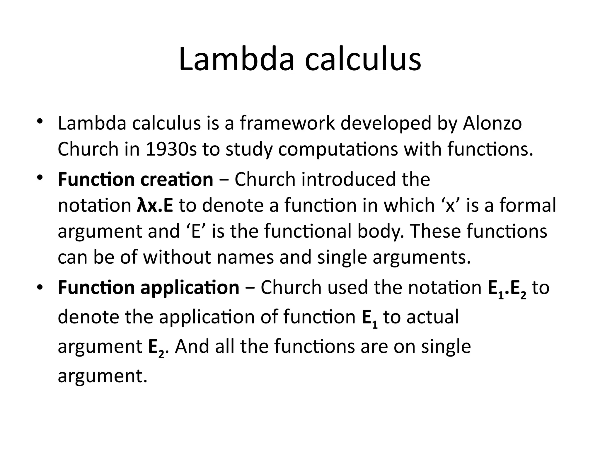
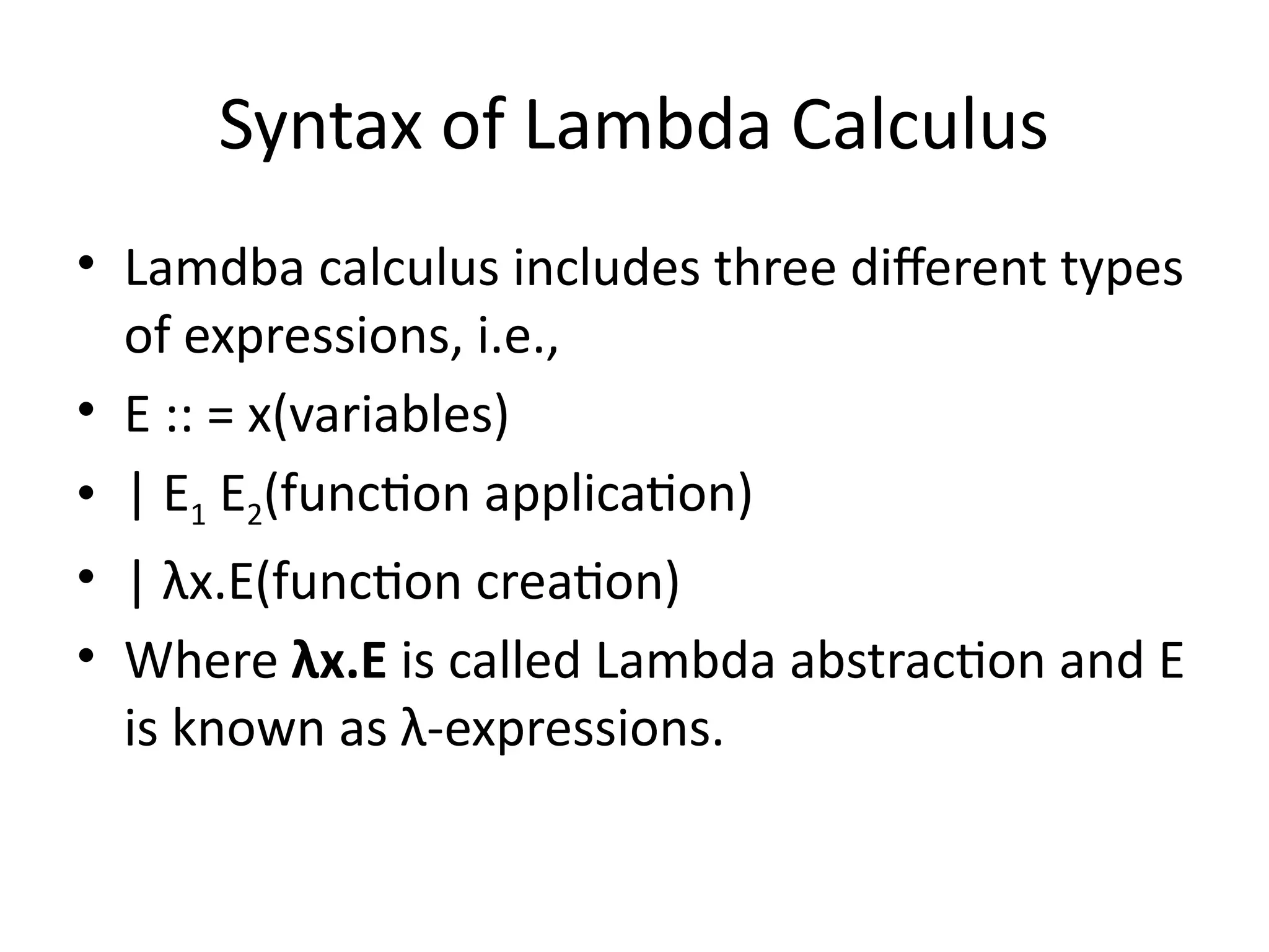
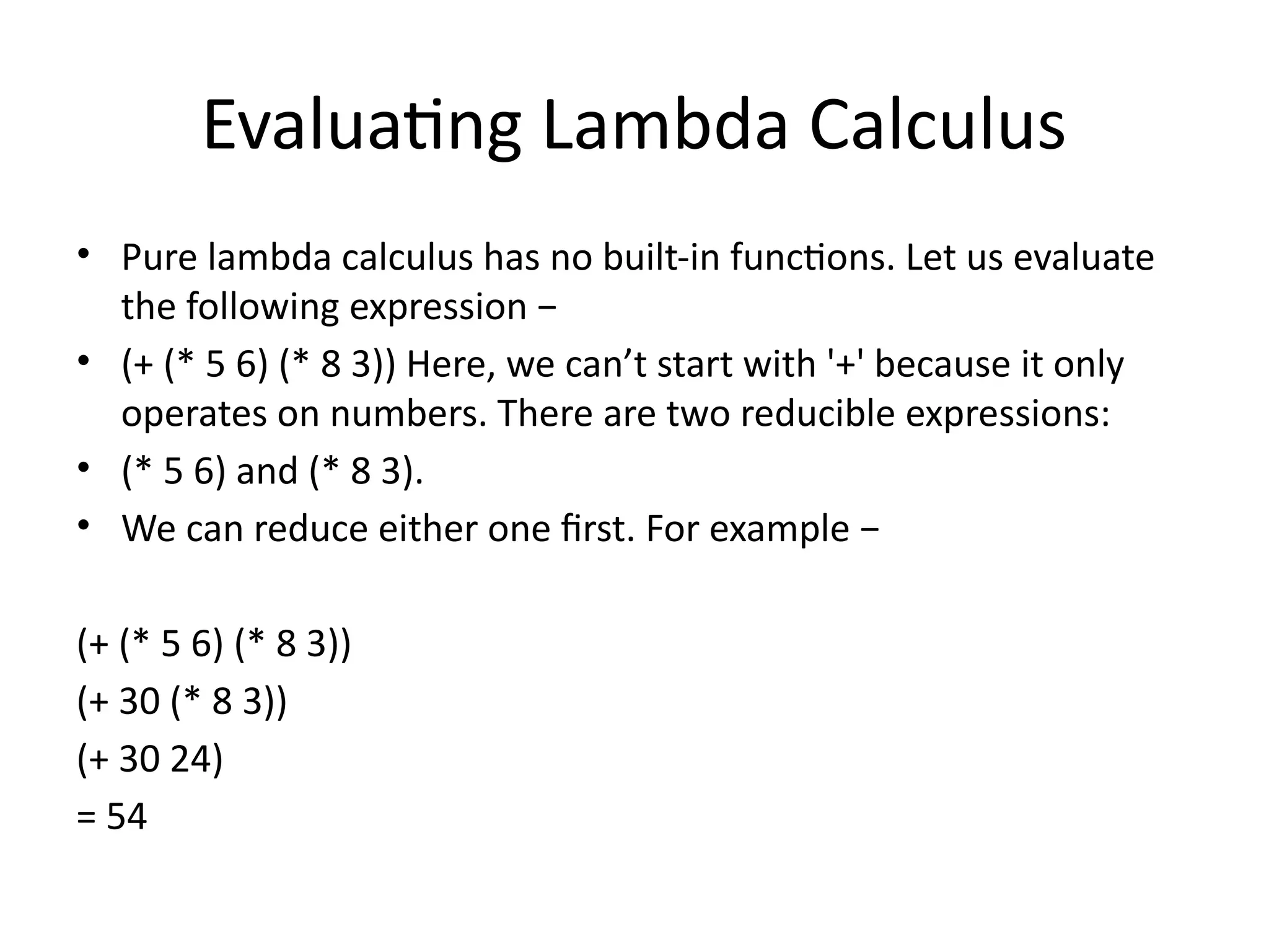
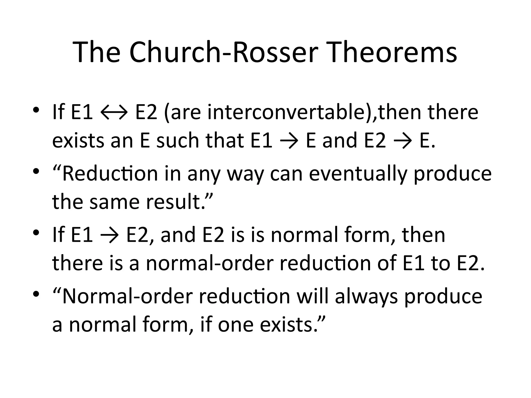
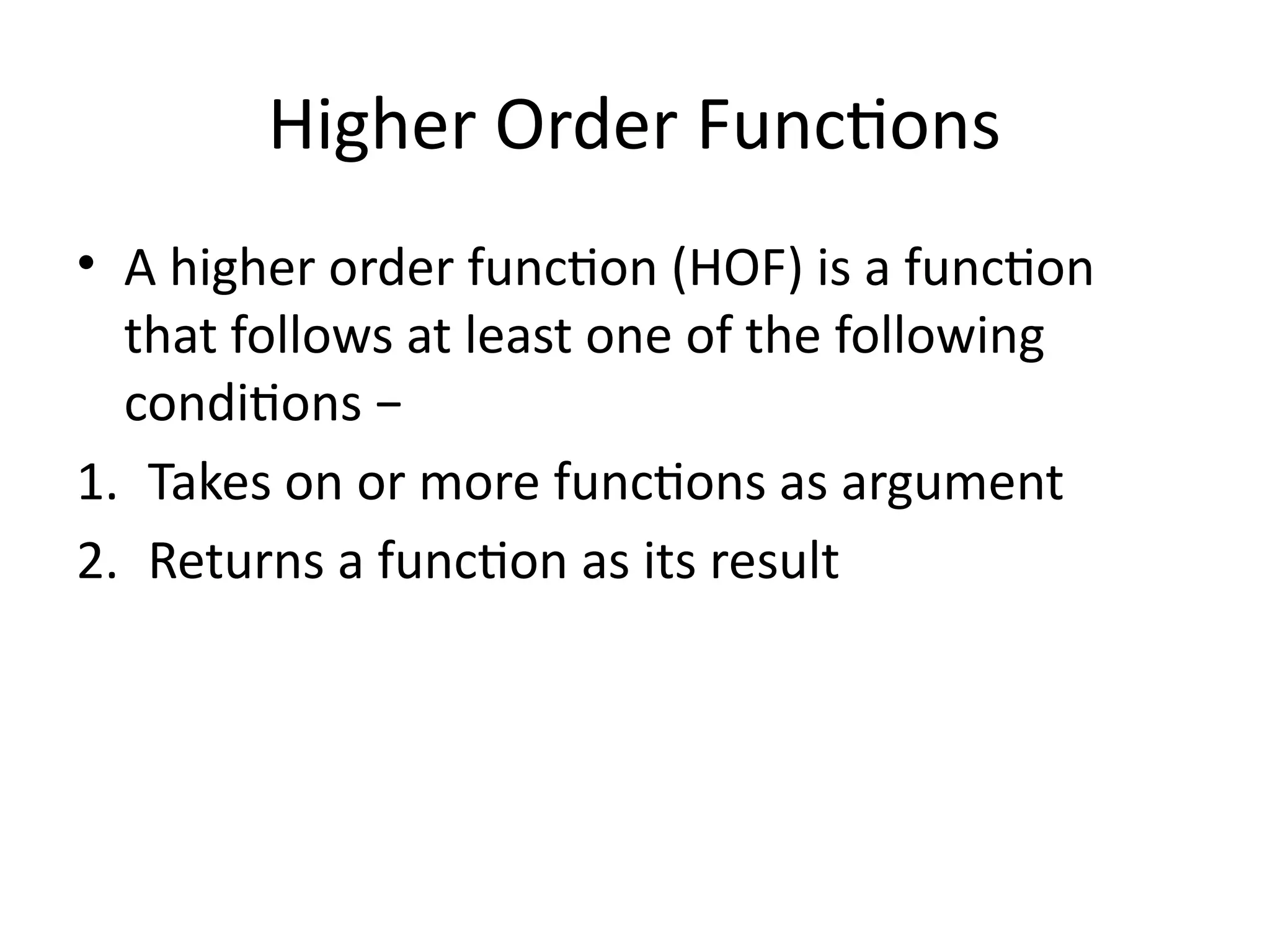
A higher-order function (HOF) is defined by its ability to take functions as arguments or return functions as results. Lazy evaluation is introduced as a strategy that delays the computation of expressions until needed, optimizing memory and performance, with both advantages and disadvantages discussed. The document also contrasts functional programming with object-oriented programming, emphasizes lambda calculus, and explains evaluation techniques including alpha, beta, and eta reductions.


![Declarative Programming Paradigm:
Functional Programming
Topics to be covered in this module: (Total Hrs: 7)
• Introduction to Lambda Calculus (1 Hr)
• Functional Programming Concepts, (2 Hrs)
• Evaluation order, Higher order functions, (2 Hrs)
• I/O- Streams (1 Hr)
• Monads (1 Hr)
Text Book :
1. Graham Hutton, Programming in Haskell, 2nd Edition, Cambridge
University Press 2016.
http://www.cs.nott.ac.uk/~pszgmh/pih.html#contents
2. Scott M L, Programming Language Pragmatics, 3rd Edn., Morgan
Kaufmann Publishers, 2009 [Chapter 10]
Other References: –
https://downloads.haskell.org/~ghc/7.8.4/docs/html/users_guide/](https://image.slidesharecdn.com/8-241118105618-bae92d26/85/8-Functional-Programming_updated-1-pptx-5-320.jpg)


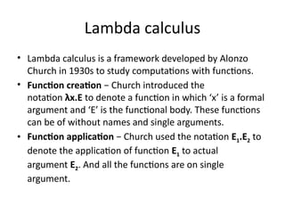


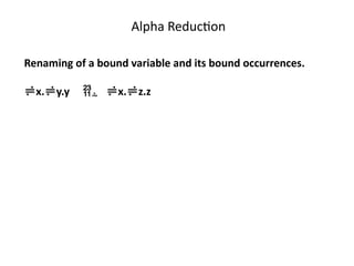
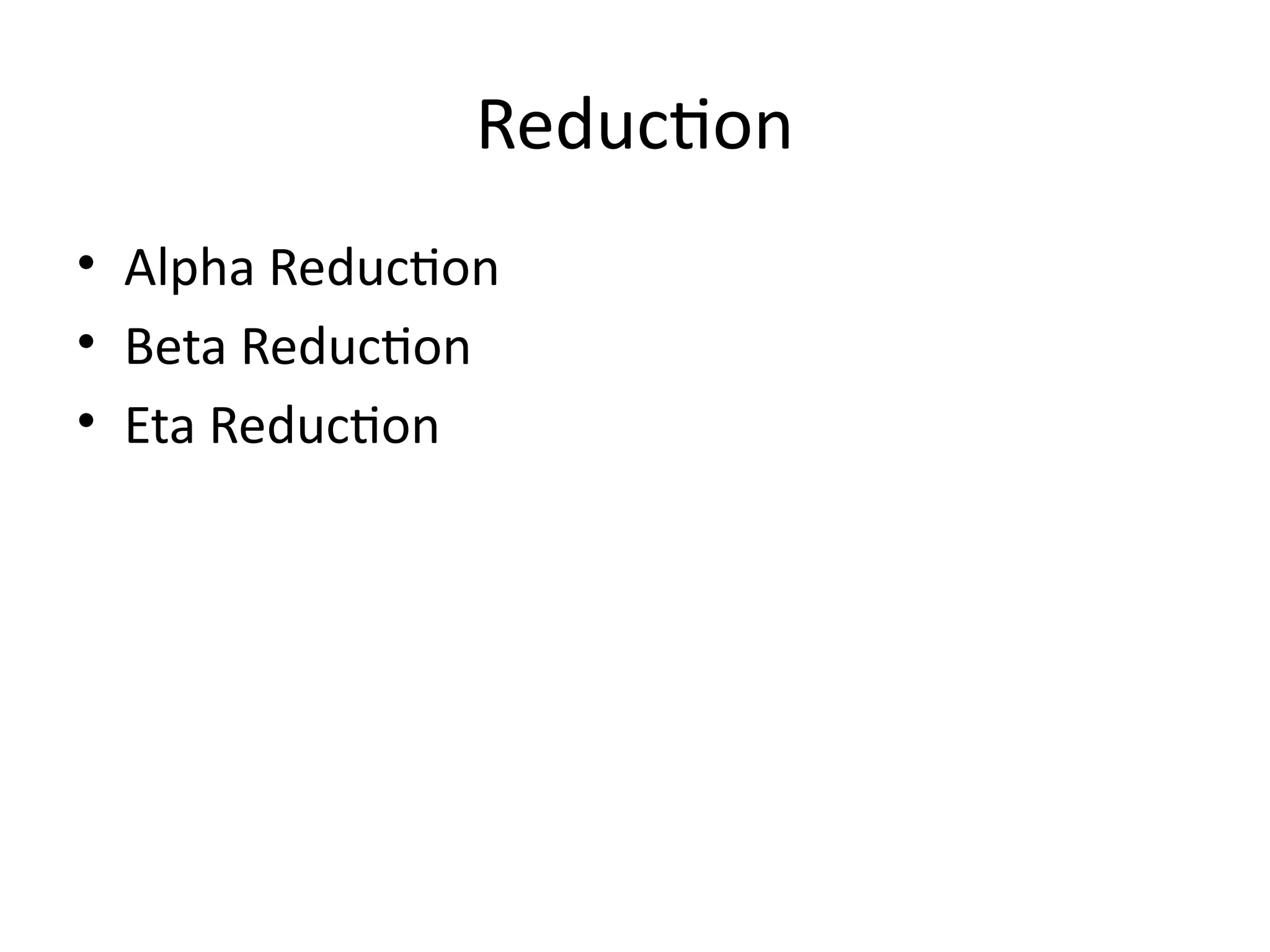
![Alpha Reduction
• If v and w are variables and E is a lambda
expression,
• λv . E α λw . E[v→w]
⇒
• provided that w does not occur at all in E,
which makes the substitution E[v→w] safe.](https://image.slidesharecdn.com/8-241118105618-bae92d26/85/8-Functional-Programming_updated-1-pptx-24-320.jpg)

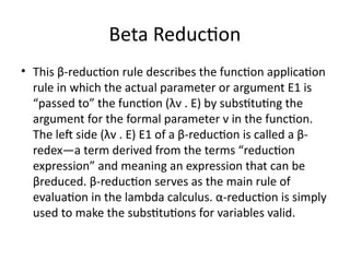
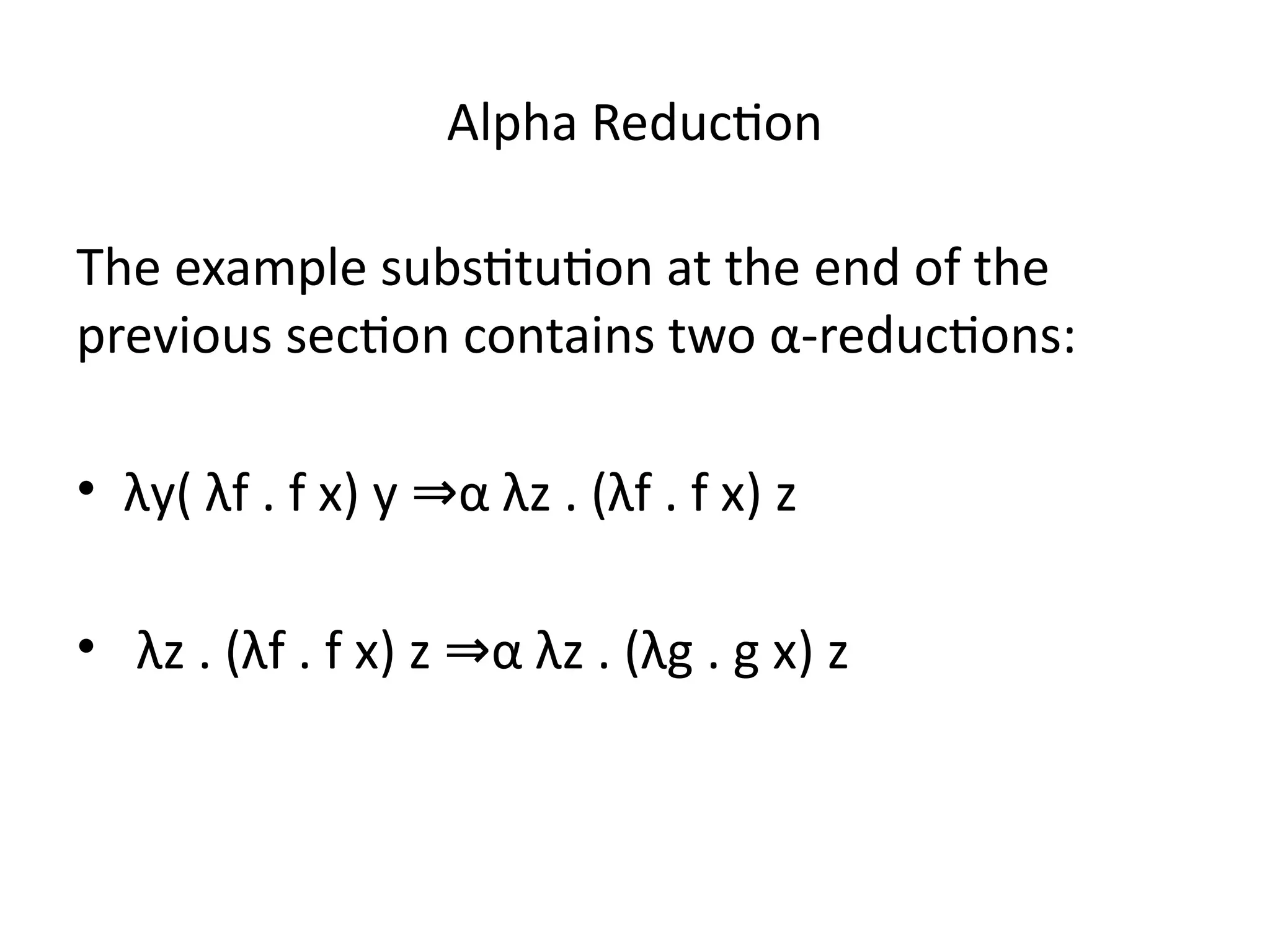
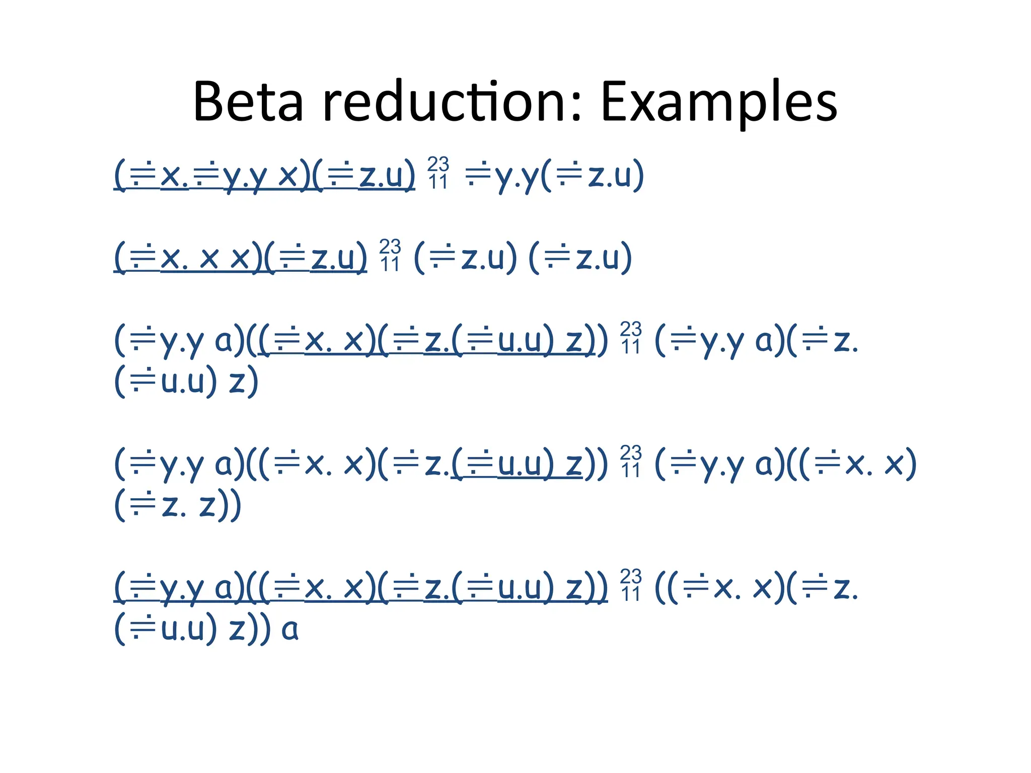
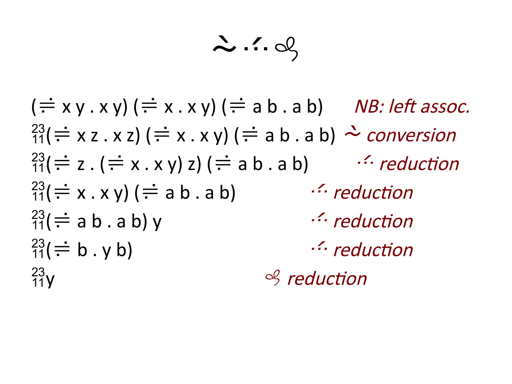
![Beta Reduction
• If v is a variable and E and E1 are lambda
expressions,
• (λv . E) E1 β E[v→E1]
⇒
• provided that the substitution E[v→E1] is
carried out according to the rules for a safe
substitution.](https://image.slidesharecdn.com/8-241118105618-bae92d26/85/8-Functional-Programming_updated-1-pptx-26-320.jpg)


![Declarative Programming Paradigm:
Functional Programming
Topics to be covered in this module: (Total Hrs: 7)
• Introduction to Lambda Calculus (1 Hr)
• Functional Programming Concepts, (2 Hrs)
• Evaluation order, Higher order functions, (2 Hrs)
• I/O- Streams (1 Hr)
• Monads (1 Hr)
Text Book :
1. Graham Hutton, Programming in Haskell, 2nd Edition, Cambridge
University Press 2016.
http://www.cs.nott.ac.uk/~pszgmh/pih.html#contents
2. Scott M L, Programming Language Pragmatics, 3rd Edn., Morgan
Kaufmann Publishers, 2009 [Chapter 10]
Other References: –
https://downloads.haskell.org/~ghc/7.8.4/docs/html/users_guide/](https://image.slidesharecdn.com/8-241118105618-bae92d26/75/8-Functional-Programming_updated-1-pptx-5-2048.jpg)


![Alpha Reduction
• If v and w are variables and E is a lambda
expression,
• λv . E α λw . E[v→w]
⇒
• provided that w does not occur at all in E,
which makes the substitution E[v→w] safe.](https://image.slidesharecdn.com/8-241118105618-bae92d26/75/8-Functional-Programming_updated-1-pptx-24-2048.jpg)
![Beta Reduction
• If v is a variable and E and E1 are lambda
expressions,
• (λv . E) E1 β E[v→E1]
⇒
• provided that the substitution E[v→E1] is
carried out according to the rules for a safe
substitution.](https://image.slidesharecdn.com/8-241118105618-bae92d26/75/8-Functional-Programming_updated-1-pptx-26-2048.jpg)


![[FLOLAC'14][scm] Functional Programming Using Haskell](https://cdn.slidesharecdn.com/ss_thumbnails/slides-140630030216-phpapp01-thumbnail.jpg?width=600ounds&width=560&fit=bounds)


