David Luebke 2
10/08/25
SortingSo Far
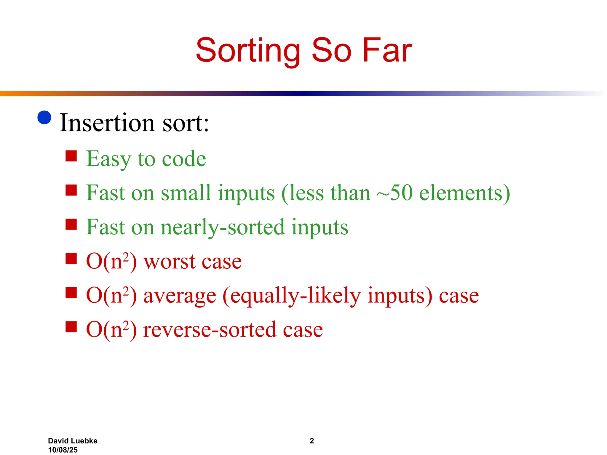
Insertion sort:
Easy to code
Fast on small inputs (less than ~50 elements)
Fast on nearly-sorted inputs
O(n2
) worst case
O(n2
) average (equally-likely inputs) case
O(n2
) reverse-sorted case
3.
David Luebke 3
10/08/25
SortingSo Far
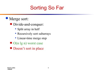
Merge sort:
Divide-and-conquer:
Split array in half
Recursively sort subarrays
Linear-time merge step
O(n lg n) worst case
Doesn’t sort in place
4.
David Luebke 4
10/08/25
SortingSo Far
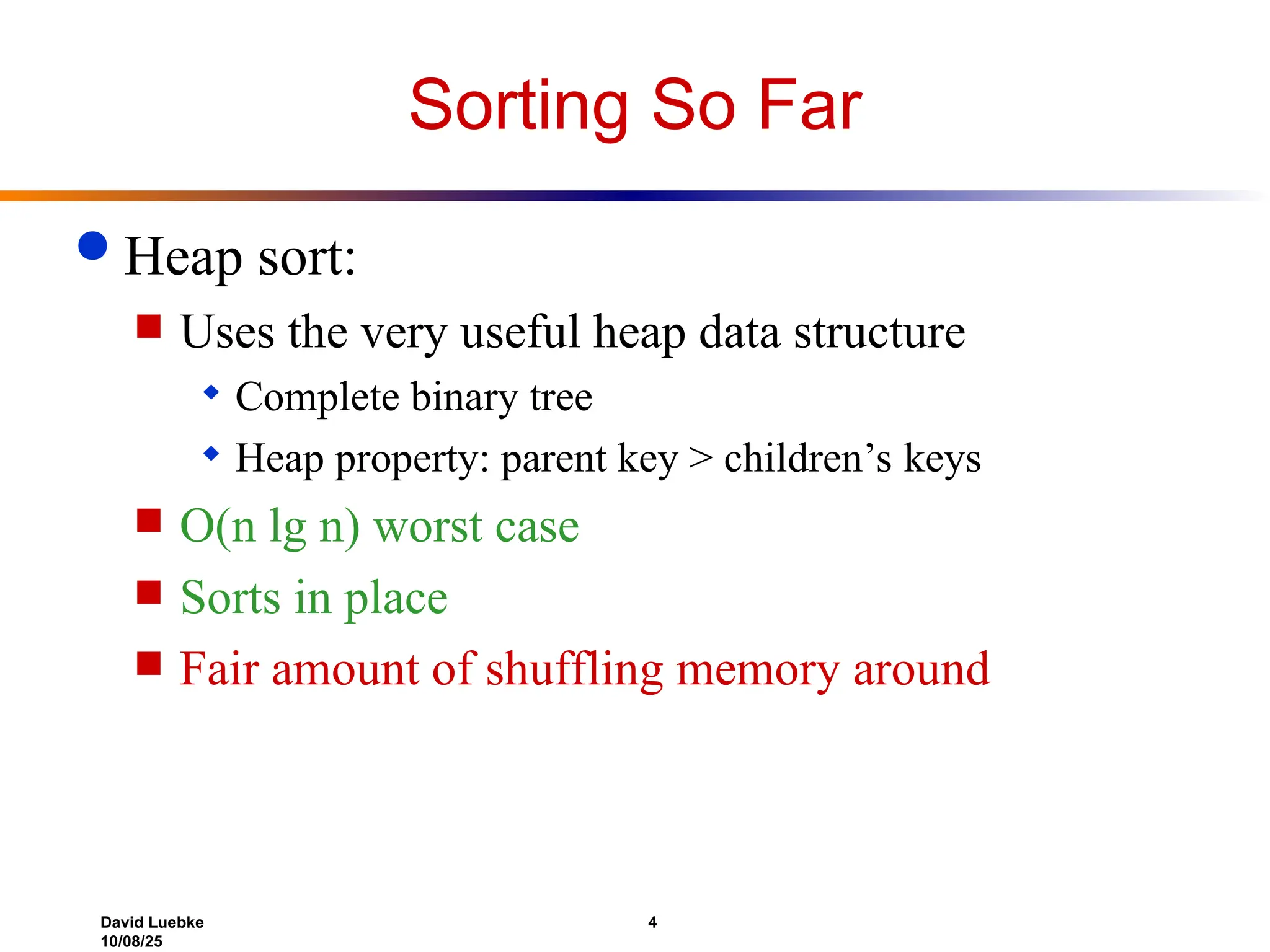
Heap sort:
Uses the very useful heap data structure
Complete binary tree
Heap property: parent key > children’s keys
O(n lg n) worst case
Sorts in place
Fair amount of shuffling memory around
5.
David Luebke 5
10/08/25
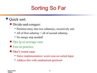
SortingSo Far
Quick sort:
Divide-and-conquer:
Partition array into two subarrays, recursively sort
All of first subarray < all of second subarray
No merge step needed!
O(n lg n) average case
Fast in practice
O(n2
) worst case
Naïve implementation: worst case on sorted input
Address this with randomized quicksort
6.
David Luebke 6
10/08/25
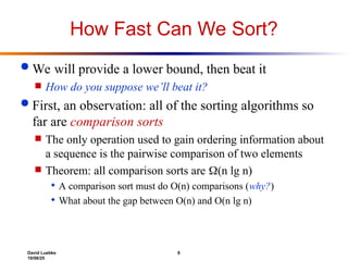
HowFast Can We Sort?
We will provide a lower bound, then beat it
How do you suppose we’ll beat it?
First, an observation: all of the sorting algorithms so
far are comparison sorts
The only operation used to gain ordering information about
a sequence is the pairwise comparison of two elements
Theorem: all comparison sorts are (n lg n)
A comparison sort must do O(n) comparisons (why?)
What about the gap between O(n) and O(n lg n)
7.
David Luebke 7
10/08/25
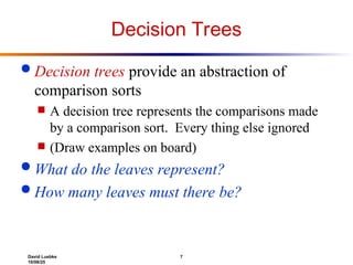
DecisionTrees
Decision trees provide an abstraction of
comparison sorts
A decision tree represents the comparisons made
by a comparison sort. Every thing else ignored
(Draw examples on board)
What do the leaves represent?
How many leaves must there be?
8.
David Luebke 8
10/08/25
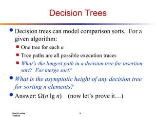
DecisionTrees
Decision trees can model comparison sorts. For a
given algorithm:
One tree for each n
Tree paths are all possible execution traces
What’s the longest path in a decision tree for insertion
sort? For merge sort?
What is the asymptotic height of any decision tree
for sorting n elements?
Answer: (n lg n) (now let’s prove it…)
9.
David Luebke 9
10/08/25
LowerBound For
Comparison Sorting
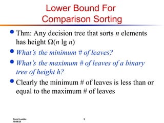
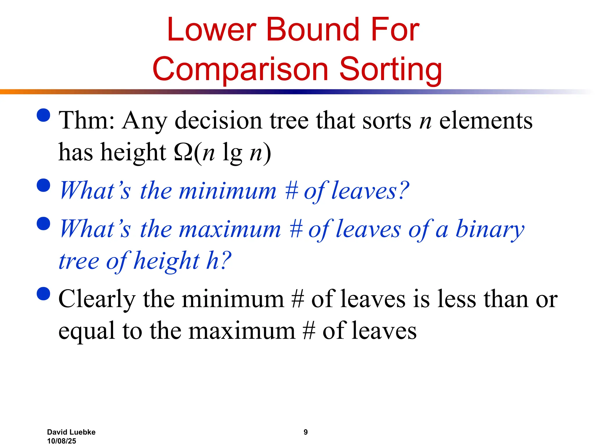
Thm: Any decision tree that sorts n elements
has height (n lg n)
What’s the minimum # of leaves?
What’s the maximum # of leaves of a binary
tree of height h?
Clearly the minimum # of leaves is less than or
equal to the maximum # of leaves
10.
David Luebke 10
10/08/25
LowerBound For
Comparison Sorting
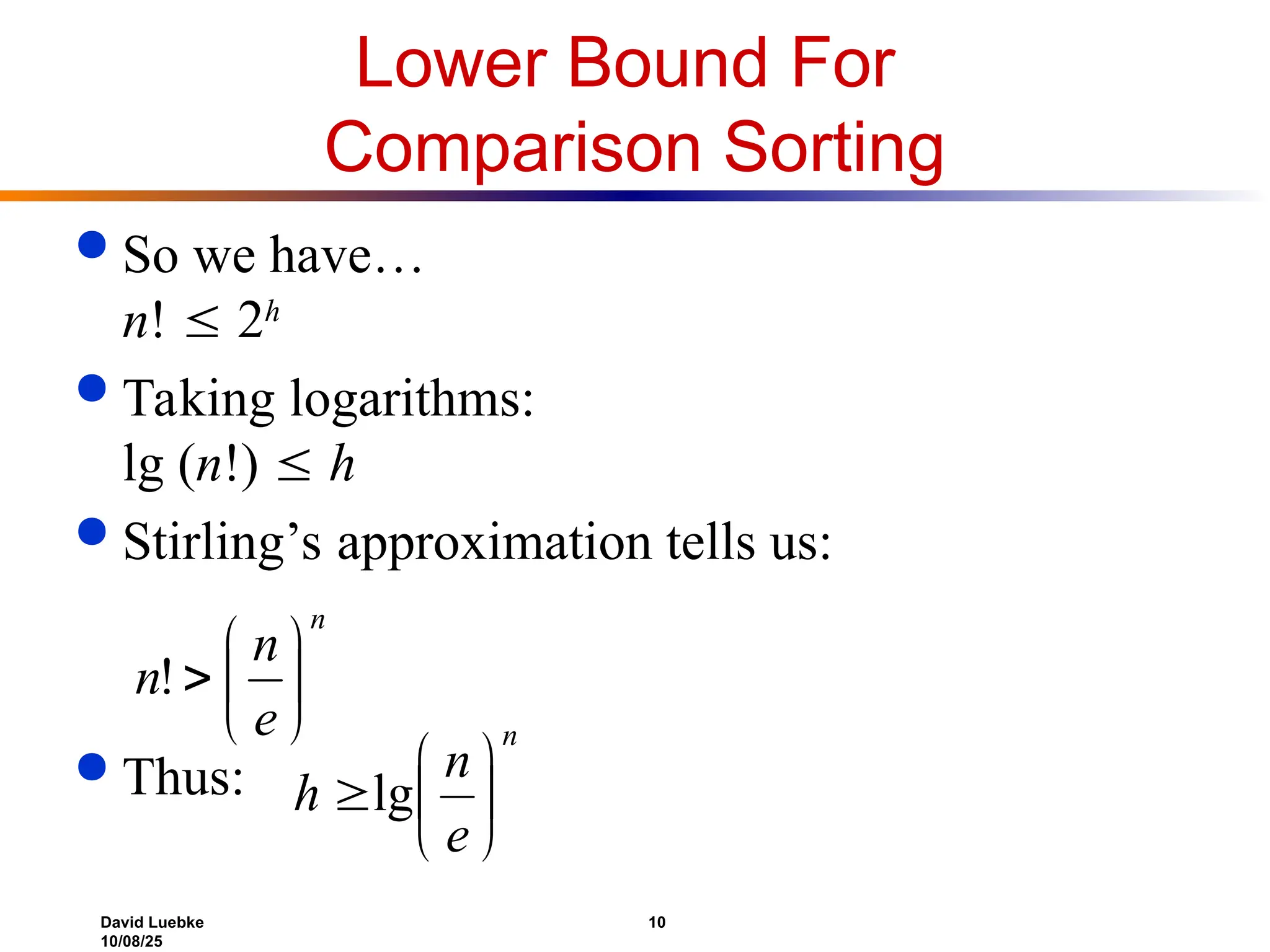
So we have…
n! 2h
Taking logarithms:
lg (n!) h
Stirling’s approximation tells us:
Thus:
n
e
n
n
!
n
e
n
h
lg
11.
David Luebke 11
10/08/25
LowerBound For
Comparison Sorting
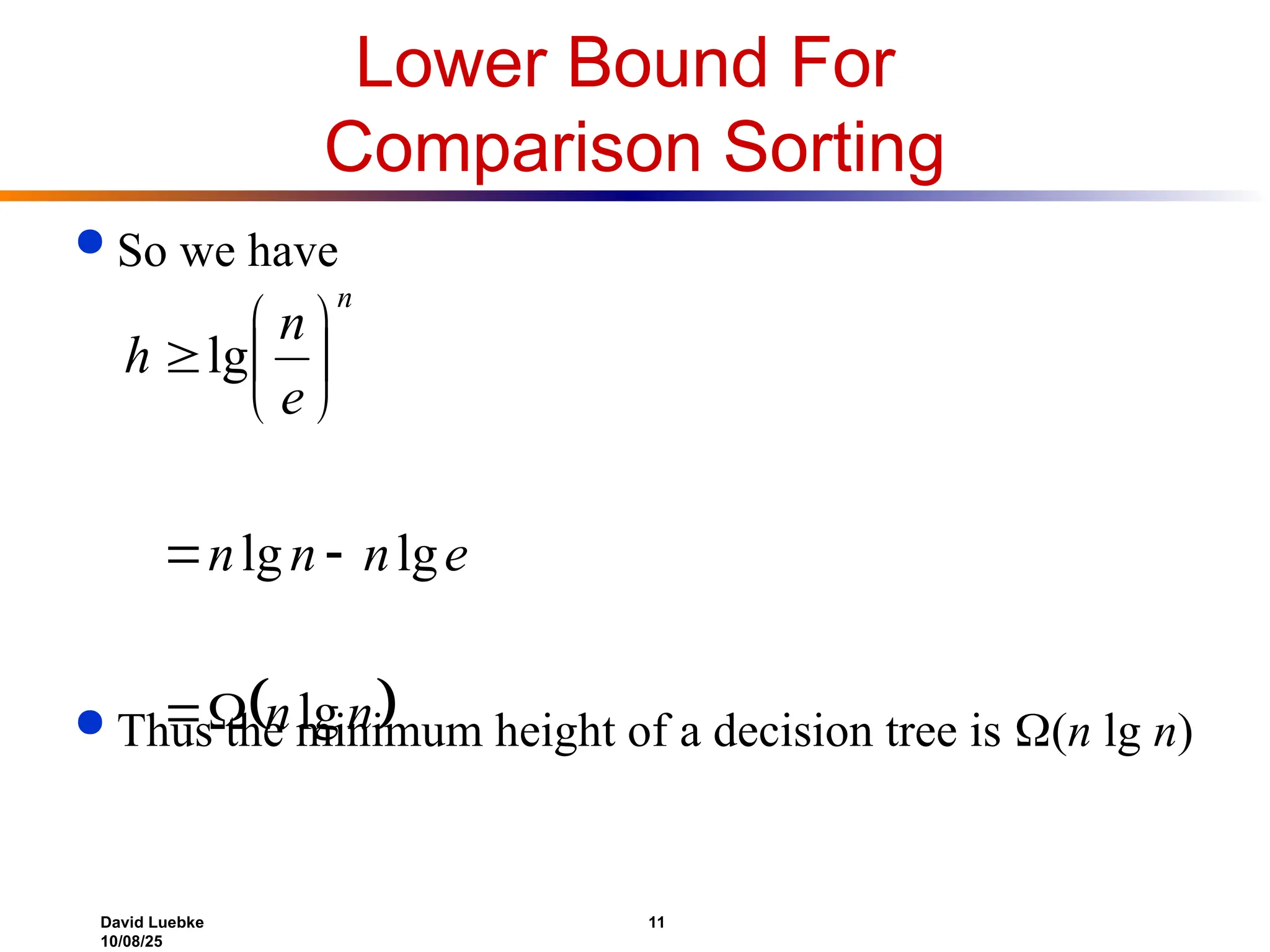
So we have
Thus the minimum height of a decision tree is (n lg n)
n
n
e
n
n
n
e
n
h
n
lg
lg
lg
lg
12.
David Luebke 12
10/08/25
LowerBound For
Comparison Sorts
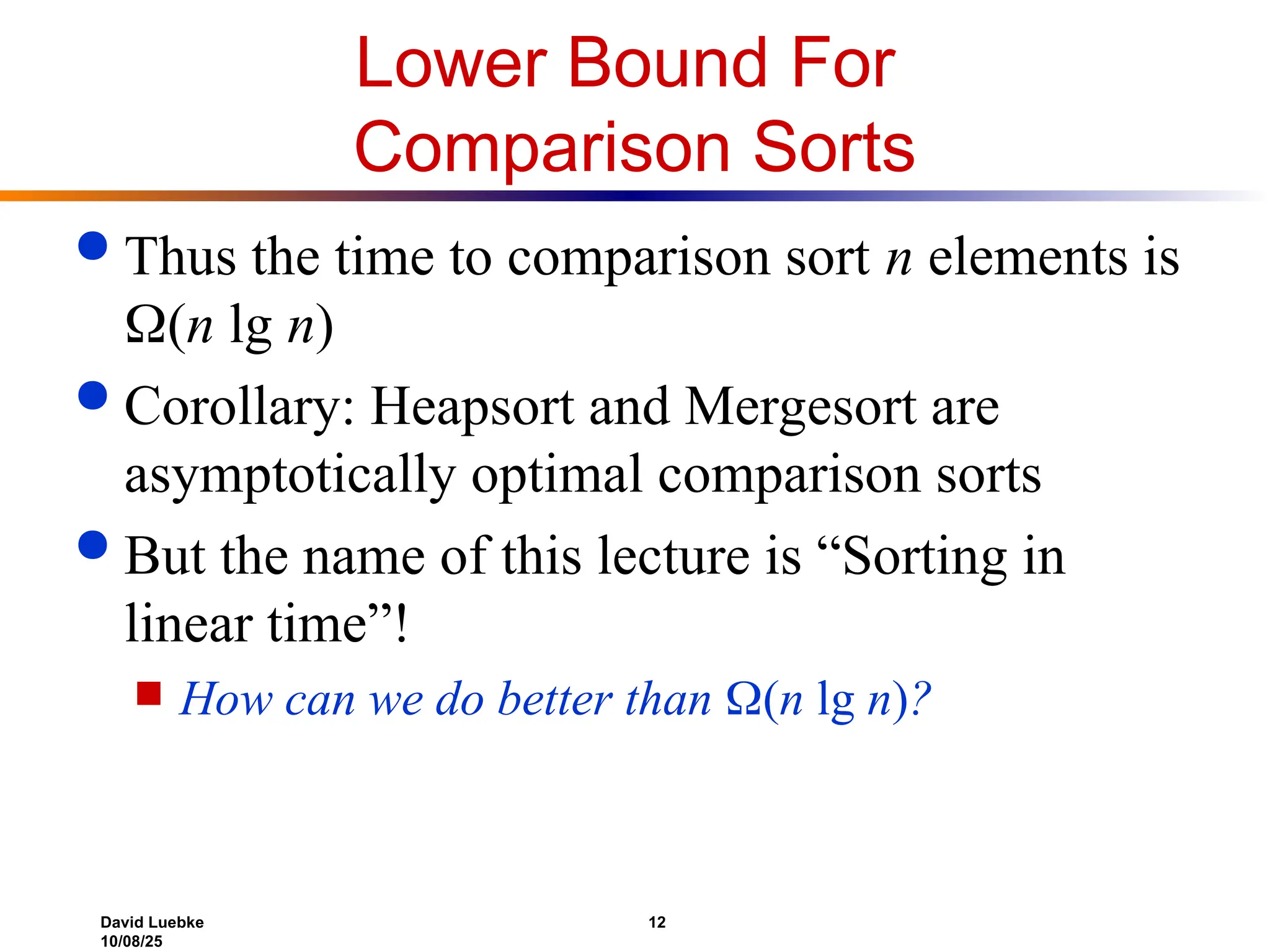
Thus the time to comparison sort n elements is
(n lg n)
Corollary: Heapsort and Mergesort are
asymptotically optimal comparison sorts
But the name of this lecture is “Sorting in
linear time”!
How can we do better than (n lg n)?
13.
David Luebke 13
10/08/25
SortingIn Linear Time
Counting sort
No comparisons between elements!
But…depends on assumption about the numbers
being sorted
We assume numbers are in the range 1.. k
The algorithm:
Input: A[1..n], where A[j] {1, 2, 3, …, k}
Output: B[1..n], sorted (notice: not sorting in place)
Also: Array C[1..k] for auxiliary storage
14.
David Luebke 14
10/08/25
CountingSort
1 CountingSort(A, B, k)
2 for i=1 to k
3 C[i]= 0;
4 for j=1 to n
5 C[A[j]] += 1;
6 for i=2 to k
7 C[i] = C[i] + C[i-1];
8 for j=n downto 1
9 B[C[A[j]]] = A[j];
10 C[A[j]] -= 1;
Work through example: A={4 1 3 4 3}, k = 4
15.
David Luebke 15
10/08/25
CountingSort
1 CountingSort(A, B, k)
2 for i=1 to k
3 C[i]= 0;
4 for j=1 to n
5 C[A[j]] += 1;
6 for i=2 to k
7 C[i] = C[i] + C[i-1];
8 for j=n downto 1
9 B[C[A[j]]] = A[j];
10 C[A[j]] -= 1;
What will be the running time?
Takes time O(k)
Takes time O(n)
16.
David Luebke 16
10/08/25
CountingSort
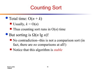
Total time: O(n + k)
Usually, k = O(n)
Thus counting sort runs in O(n) time
But sorting is (n lg n)!
No contradiction--this is not a comparison sort (in
fact, there are no comparisons at all!)
Notice that this algorithm is stable
17.
David Luebke 17
10/08/25
CountingSort
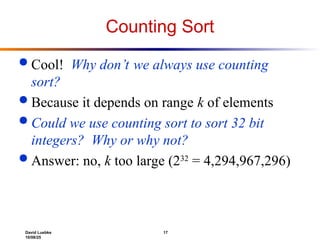
Cool! Why don’t we always use counting
sort?
Because it depends on range k of elements
Could we use counting sort to sort 32 bit
integers? Why or why not?
Answer: no, k too large (232
= 4,294,967,296)
18.
David Luebke 18
10/08/25
CountingSort
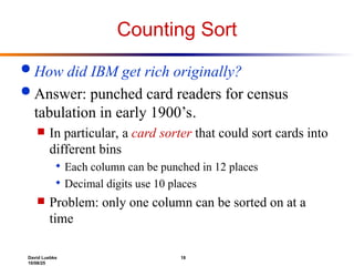
How did IBM get rich originally?
Answer: punched card readers for census
tabulation in early 1900’s.
In particular, a card sorter that could sort cards into
different bins
Each column can be punched in 12 places
Decimal digits use 10 places
Problem: only one column can be sorted on at a
time
19.
David Luebke 19
10/08/25
RadixSort
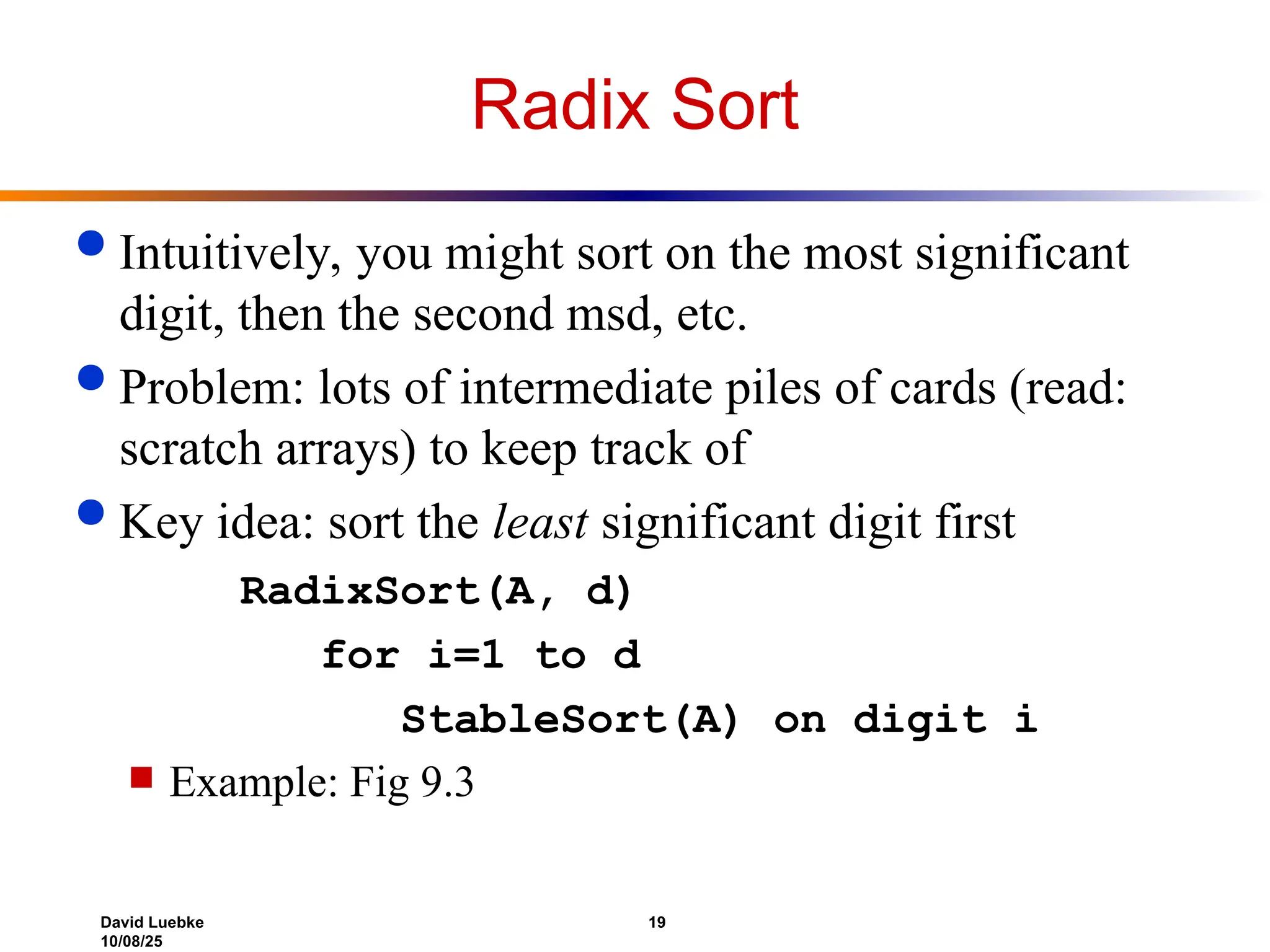
Intuitively, you might sort on the most significant
digit, then the second msd, etc.
Problem: lots of intermediate piles of cards (read:
scratch arrays) to keep track of
Key idea: sort the least significant digit first
RadixSort(A, d)
for i=1 to d
StableSort(A) on digit i
Example: Fig 9.3
20.
David Luebke 20
10/08/25
RadixSort
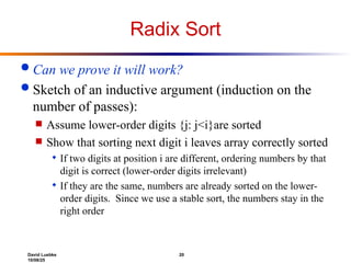
Can we prove it will work?
Sketch of an inductive argument (induction on the
number of passes):
Assume lower-order digits {j: j<i}are sorted
Show that sorting next digit i leaves array correctly sorted
If two digits at position i are different, ordering numbers by that
digit is correct (lower-order digits irrelevant)
If they are the same, numbers are already sorted on the lower-
order digits. Since we use a stable sort, the numbers stay in the
right order
21.
David Luebke 21
10/08/25
RadixSort
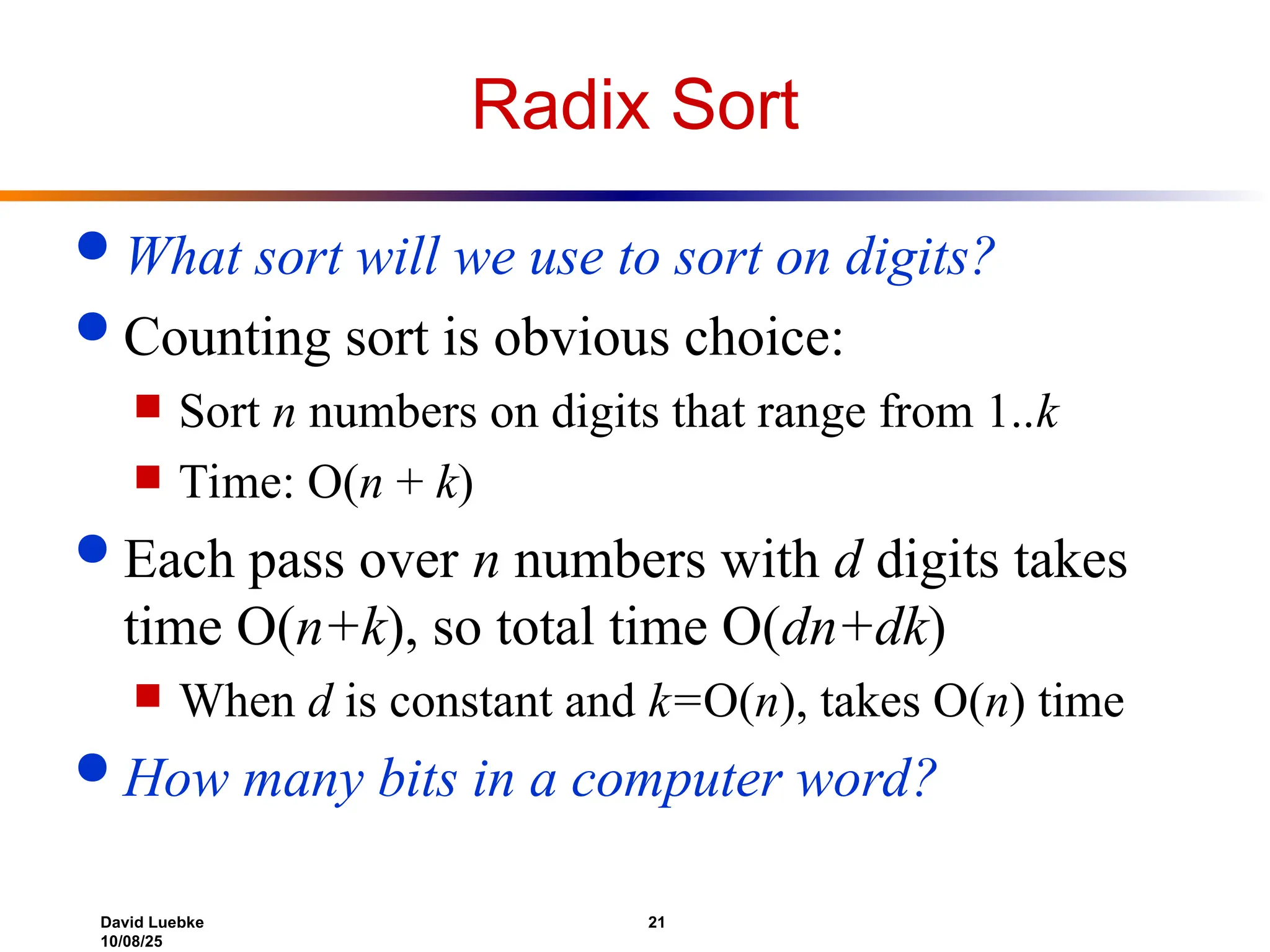
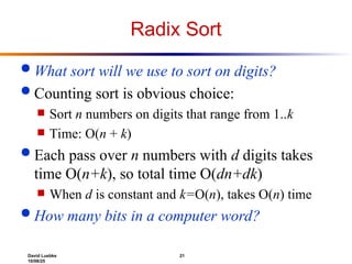
What sort will we use to sort on digits?
Counting sort is obvious choice:
Sort n numbers on digits that range from 1..k
Time: O(n + k)
Each pass over n numbers with d digits takes
time O(n+k), so total time O(dn+dk)
When d is constant and k=O(n), takes O(n) time
How many bits in a computer word?
22.
David Luebke 22
10/08/25
RadixSort
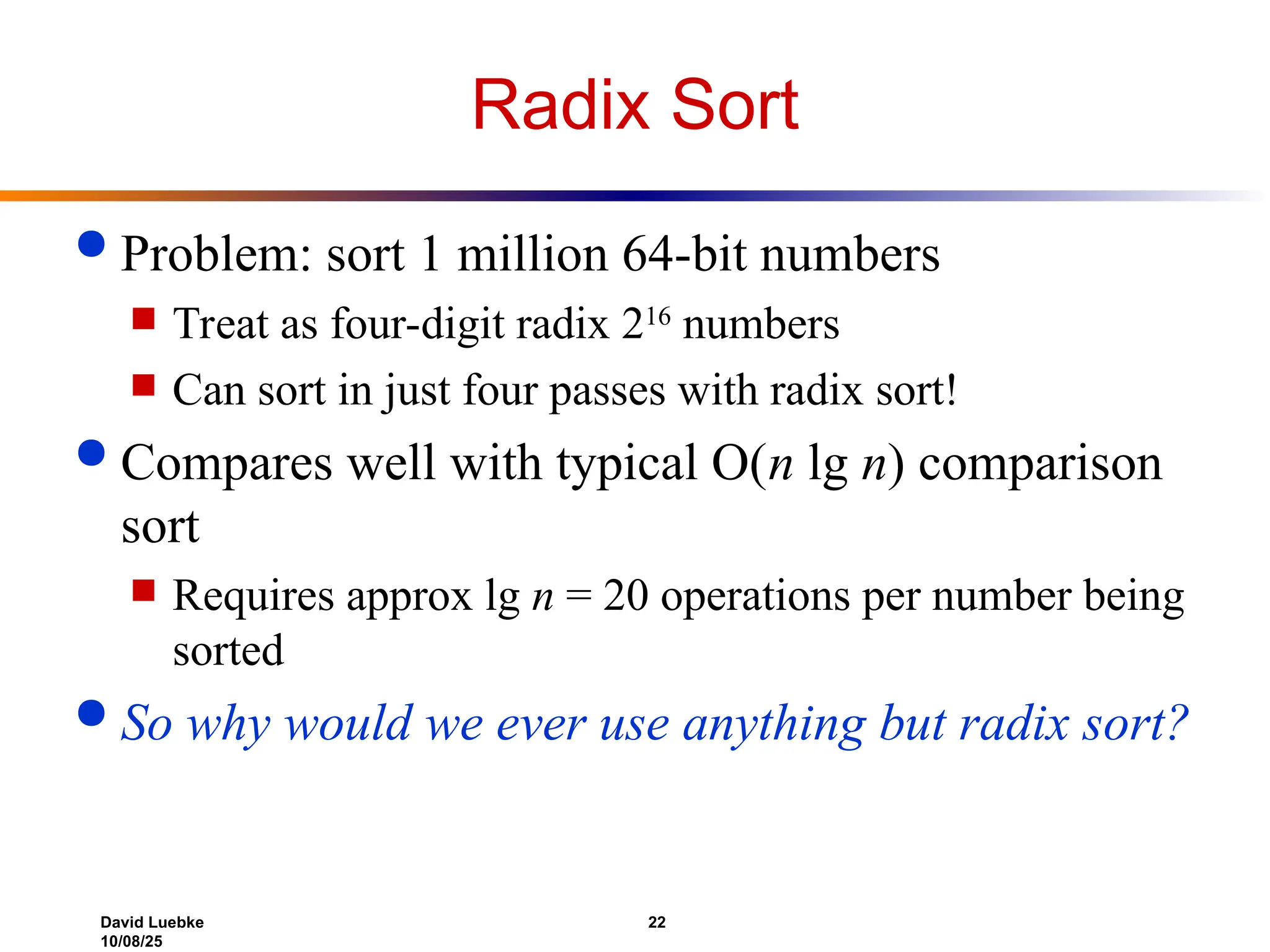
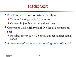
Problem: sort 1 million 64-bit numbers
Treat as four-digit radix 216
numbers
Can sort in just four passes with radix sort!
Compares well with typical O(n lg n) comparison
sort
Requires approx lg n = 20 operations per number being
sorted
So why would we ever use anything but radix sort?
23.
David Luebke 23
10/08/25
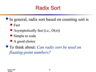
RadixSort
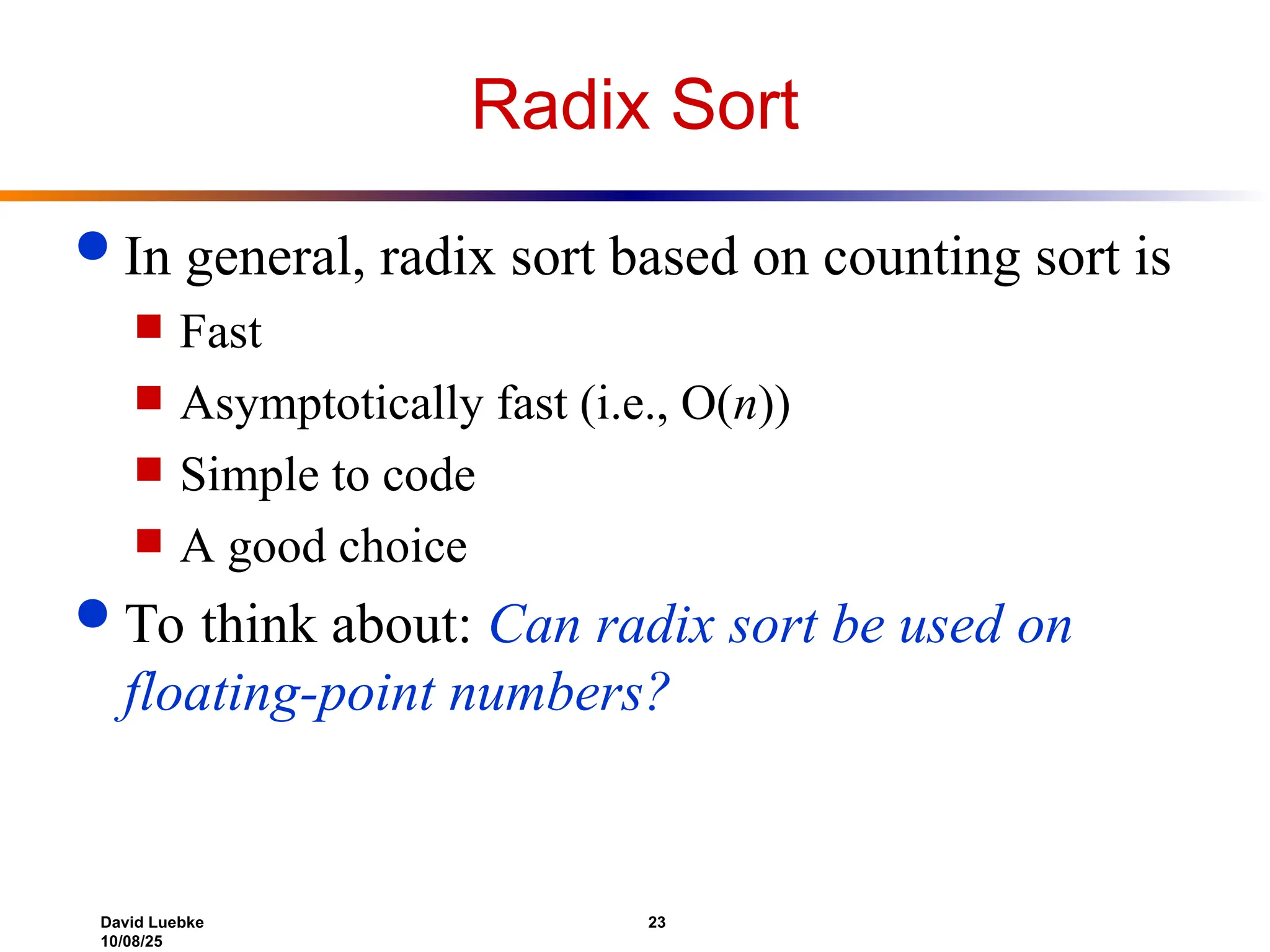
In general, radix sort based on counting sort is
Fast
Asymptotically fast (i.e., O(n))
Simple to code
A good choice
To think about: Can radix sort be used on
floating-point numbers?


![David Luebke 13
10/08/25
Sorting In Linear Time
Counting sort
No comparisons between elements!
But…depends on assumption about the numbers
being sorted
We assume numbers are in the range 1.. k
The algorithm:
Input: A[1..n], where A[j] {1, 2, 3, …, k}
Output: B[1..n], sorted (notice: not sorting in place)
Also: Array C[1..k] for auxiliary storage](https://image.slidesharecdn.com/lecture9-251008051839-5ad180e7/85/Linear-Time-Sorting-Algorithm-Functionality-13-320.jpg)
![David Luebke 14
10/08/25
Counting Sort
1 CountingSort(A, B, k)
2 for i=1 to k
3 C[i]= 0;
4 for j=1 to n
5 C[A[j]] += 1;
6 for i=2 to k
7 C[i] = C[i] + C[i-1];
8 for j=n downto 1
9 B[C[A[j]]] = A[j];
10 C[A[j]] -= 1;
Work through example: A={4 1 3 4 3}, k = 4](https://image.slidesharecdn.com/lecture9-251008051839-5ad180e7/85/Linear-Time-Sorting-Algorithm-Functionality-14-320.jpg)
![David Luebke 15
10/08/25
Counting Sort
1 CountingSort(A, B, k)
2 for i=1 to k
3 C[i]= 0;
4 for j=1 to n
5 C[A[j]] += 1;
6 for i=2 to k
7 C[i] = C[i] + C[i-1];
8 for j=n downto 1
9 B[C[A[j]]] = A[j];
10 C[A[j]] -= 1;
What will be the running time?
Takes time O(k)
Takes time O(n)](https://image.slidesharecdn.com/lecture9-251008051839-5ad180e7/85/Linear-Time-Sorting-Algorithm-Functionality-15-320.jpg)


![David Luebke 13
10/08/25
Sorting In Linear Time
Counting sort
No comparisons between elements!
But…depends on assumption about the numbers
being sorted
We assume numbers are in the range 1.. k
The algorithm:
Input: A[1..n], where A[j] {1, 2, 3, …, k}
Output: B[1..n], sorted (notice: not sorting in place)
Also: Array C[1..k] for auxiliary storage](https://image.slidesharecdn.com/lecture9-251008051839-5ad180e7/75/Linear-Time-Sorting-Algorithm-Functionality-13-2048.jpg)
![David Luebke 14
10/08/25
Counting Sort
1 CountingSort(A, B, k)
2 for i=1 to k
3 C[i]= 0;
4 for j=1 to n
5 C[A[j]] += 1;
6 for i=2 to k
7 C[i] = C[i] + C[i-1];
8 for j=n downto 1
9 B[C[A[j]]] = A[j];
10 C[A[j]] -= 1;
Work through example: A={4 1 3 4 3}, k = 4](https://image.slidesharecdn.com/lecture9-251008051839-5ad180e7/75/Linear-Time-Sorting-Algorithm-Functionality-14-2048.jpg)
![David Luebke 15
10/08/25
Counting Sort
1 CountingSort(A, B, k)
2 for i=1 to k
3 C[i]= 0;
4 for j=1 to n
5 C[A[j]] += 1;
6 for i=2 to k
7 C[i] = C[i] + C[i-1];
8 for j=n downto 1
9 B[C[A[j]]] = A[j];
10 C[A[j]] -= 1;
What will be the running time?
Takes time O(k)
Takes time O(n)](https://image.slidesharecdn.com/lecture9-251008051839-5ad180e7/75/Linear-Time-Sorting-Algorithm-Functionality-15-2048.jpg)