Big Picture
• Introductionto Python libraries- Pandas, Matplotlib.
• Data structures in Pandas - Series and Data Frames.
• Series: Creation of Series from – ndarray, dictionary, scalar value;
mathematical operations; Head and Tail functions; Selection, Indexing and
Slicing.
• Data Frames:
• Text/CSV files
• Operations on rows and columns: add, select, delete, rename;
• Head and Tail functions;
• Indexing using Labels, Boolean Indexing;
• Importing/Exporting Data between CSV files and Data Frames.
3.
PRETEST
1. In lists,you can change the elements of a list in place.
(True/False)
2. The _______ brackets are used to enclose the values of a list.
3. l1= list(‘ClassXI’) returns :
4. The position of each element in the list is considered as
___________.
5. The property which changes the element of a list in place
but not changes the memory address is known as
__________.
4.
Computer Science hasbeen a field of continuous evolution and regular
advancements in terms of software efficiency, programming
methodologies and applications.
With the advent of data sciences or data analytics, it has become
easier and efficient to handle big data or huge data.
Data science is a large field covering everything from data collection,
cleaning, standardization, analysis, visualization and reporting.
INTRODUCTION
5.
DATA PROCESSING
Data processingis an important part of analyzing the data because the
data is not always available in the desired format.
Various processing are required before analyzing the data such as
cleaning, restructuring or merging etc.
NumPy, Spicy, Cython, Panda are the tools available in Python which
can be used for fast processing of data.
6.
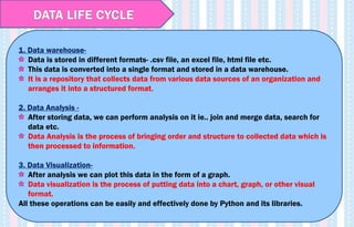
DATA LIFE CYCLE
1.Data warehouse-
Data is stored in different formats- .csv file, an excel file, html file etc.
This data is converted into a single format and stored in a data warehouse.
It is a repository that collects data from various data sources of an organization and
arranges it into a structured format.
2. Data Analysis -
After storing data, we can perform analysis on it ie.. join and merge data, search for
data etc.
Data Analysis is the process of bringing order and structure to collected data which is
then processed to information.
3. Data Visualization-
After analysis we can plot this data in the form of a graph.
Data visualization is the process of putting data into a chart, graph, or other visual
format.
All these operations can be easily and effectively done by Python and its libraries.
Python library isa collection of functions and methods which can be
used to perform any functions without writing your code.
Pandas is built on top of two core Python libraries—matplotlib for
data visualization and NumPy for mathematical operations.
Pandas acts as a wrapper over these libraries, allowing you to
access many of matplotlib's and NumPy's methods with less code.
PYTHON LIBRARIES
9.
The Pandas isa high-performance open source library for data
analysis in Python developed by Wes McKinney in 2008.
The name Pandas is derived from the word Panel Data System– an
Econometrics from Multidimensional data.
It makes data importing and data analyzing easier.
It is a most famous Python package for data science, which offers
powerful and flexible data structures that make data analysis and
manipulation easy.
Guido van Rossum
PYTHON PANDAS INTRODUCTION
10.
Pandas builds onpackages like NumPy and matplotlib to give us a
single & convenient place for data analysis and visualization work.
It is built on NumPy and its key data structure is called DataFrame
Python with Pandas is used in a wide range of fields including
academic and commercial domains including finance, economics,
Statistics, analytics, etc.
PYTHON PANDAS
11.
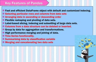
Fast and efficientDataFrame object with default and customized indexing.
Selecting particular rows and columns from data sets
Arranging data in ascending or descending order
Flexible reshaping and pivoting of data sets.
Label-based slicing, indexing and subsetting of large data sets.
Columns from a data structure can be deleted or inserted.
Group by data for aggregation and transformations.
High performance merging and joining of data.
Time Series functionality.
Summarising data by classification variable
Merging and concatenating two data sets
Key Features of Pandas
12.
Right click commandprompt Run as Administrator
Click on YES on the USER ACCESS Window to open administrator
window
Make sure of the file path before you install with pip
Change your path to the folder python 3.6
Move to installation scripts folder
When you explore the folder you will see a file pip.exe
Type pip install pandas
Note-
• A package contains all the files you need for a module.
• Modules are Python code libraries you can include in your project.
• pip is the standard package manager for Python. It allows you to install
and manage additional packages that are not part of the Python standard
library.
Installing Pandas
Pandas Datatypes :
Pandasdtype Python Type NumPy type Usage
object Str String_, unicode_ Text
int64 Int int, int8, int16, int32,
int64, uint8, uint16,
uint32, uint64
Integer
numbers
float64 Float float, float16, float32,
float64
Floating point
numbers
bool bool bool True / False
datetime64 NA datetime64[ns] Date & Time
values
15.
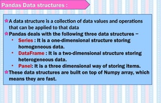
Pandas Data structures:
A data structure is a collection of data values and operations
that can be applied to that data
Pandas deals with the following three data structures −
• Series : It is a one-dimensional structure storing
homogeneous data.
• DataFrame : It is a two-dimensional structure storing
heterogeneous data.
• Panel: It is a three dimensional way of storing items.
These data structures are built on top of Numpy array, which
means they are fast.
16.
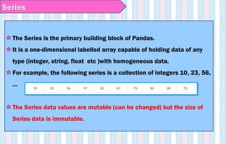
Series
The Series isthe primary building block of Pandas.
It is a one-dimensional labelled array capable of holding data of any
type (integer, string, float etc )with homogeneous data.
For example, the following series is a collection of integers 10, 23, 56,
…
The Series data values are mutable (can be changed) but the size of
Series data is immutable.
17.
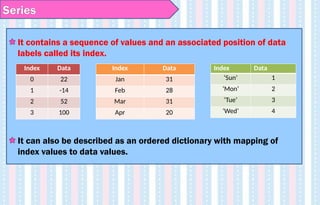
Series
It contains asequence of values and an associated position of data
labels called its index.
It can also be described as an ordered dictionary with mapping of
index values to data values.
Index Data
0 22
1 -14
2 52
3 100
Index Data
Jan 31
Feb 28
Mar 31
Apr 20
Index Data
‘Sun’ 1
‘Mon’ 2
‘Tue’ 3
‘Wed’ 4
18.
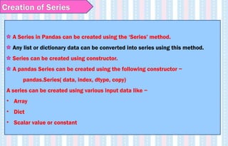
Creation of Series
ASeries in Pandas can be created using the ‘Series’ method.
Any list or dictionary data can be converted into series using this method.
Series can be created using constructor.
A pandas Series can be created using the following constructor −
pandas.Series( data, index, dtype, copy)
A series can be created using various input data like −
• Array
• Dict
• Scalar value or constant
19.
A basic series,which can be created is an Empty Series.
Example - [Here ‘s’ is the Series Object]
import pandas as pd
s = pd.Series()
print s
Its output is as follows −
Series([], dtype: float64)
Note –
• Series () displays an empty list along with its default data type.
• Pd is an alternate name given to the Pandas module. Its significance is that we
can use ‘pd’ instead of typing Pandas every time we need to use it.
• Import statement is used for loading Pandas module into the memory and can
be used to work with.
Creation of Empty Series
20.
Creating DataSeries witha list
Syntax:
<Series Object>=pandas.Series([data],index=[index])
Eg:-
import pandas as pd
s=pd.Series( [ 2,4,6,8,10])
print(s)
S- is a series variable
Series() – method displays a list along with
default data type
pd is the alternative name given to panda
module
Import statement is used to load pandas
module into the memory and can be used
21.
Program- DataSeries
>>> s=pandas.Series ( [3,-5,7,4] , index=['a','b','c','d‘] )
>>> s
Output:
a 3
b -5
c 7
d 4
dtype: int64
22.
>>> st =pd.Series([20, 70, 10], index=['frog', 'fish', 'hawk'])
>>> st
frog 20
fish 70
hawk 10
dtype: int64
>>> st.index.name = 'Animals'
>>> st
Animals
frog 20
fish 70
hawk 10
dtype: int64
Program
23.
Activity
• Create aseries having names of any five famous
monuments of India and assign their States as
index values.
24.
Think and Reflect
•While importing Pandas, is it mandatory to
always use pd as an alias name? What would
happen if we give any other name?
• Try it and write your explanation in the
notebook.
Starter
• Create alist of 7 emirates and create a series from
that with index values showing it from 1 to 7 .
29.
Think ?
• Isit possible to create a series from dictionary and
how?
• What will be the index value of that series ?
30.
Creation of seriesfrom Dictionary
• Dictionary keys can be used to construct an index for a
Series.
31.
Attribute of Series
•Series support vector operations.
• Any operation gets performed on every single element.
Eg:-
import pandas as pd
List = [5, 2, 3,7]
s1= pd.Series (List)
Guess the output of these statements:
print (list *2)
print (s1*2)
32.
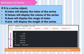
Attributes of Series
IfN is a series object,
• N.Index will display the index of the series
• N.Values will display the values of the series
• N.Axes will display the range of index
• N.size will display the length of the series
The arrow on the image displays “axis 0” and its direction for the Series object.
33.
In Python, one-dimensionalstructures are displayed as a row of
values. On the contrary, here we see that Series is displayed as a
column of values.
Each cell in Series is accessible via index value along the “axis 0”. For
our Series object indexes are: 0, 1, 2, 3, 4. Here is an example of
accessing different values:
import pandas as pd
N=pd.Series([‘Red’, ‘Green’,’Yellow’,’Orange’, Blue’])
print(N[0])
print (N.axes)
Red
[RangeIndex(start=0, stop=5, step=1)]
Axis in Series
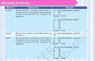
ACCESSING ROWS USINGHEAD () AND TAIL() FUNCTION
Series.head() function will display the top 5 rows in the series.
Series.tail() function will display the last 5 rows in the series
In both the functions, if a number is passed as parameter Pandas will
print the specified number of rows.
Eg:-
>>> a=pd.Series([2,4,6,8,10,12,14,16])
>>> a.head()
0 2
1 4
2 6
3 8
4 10
dtype: int64
36.
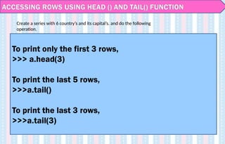
ACCESSING ROWS USINGHEAD () AND TAIL() FUNCTION
To print only the first 3 rows,
To print the last 5 rows,
To print the last 3 rows,
Create a series with 6 country’s and its capital’s as index. and do the
following operation.
37.
ACCESSING ROWS USINGHEAD () AND TAIL() FUNCTION
To print only the first 3 rows,
>>> a.head(3)
To print the last 5 rows,
>>>a.tail()
To print the last 3 rows,
>>>a.tail(3)
Create a series with 6 country’s and its capital’s. and do the following
operation.
38.
Vector operations inSeries
• Series support vector operations.
• Any operation gets performed on every single element.
Eg:-
import pandas as pd
List = [5, 2, 3,7]
s1= pd.Series (List)
Guess the output of these statements:
print (list *2)
print (s1*2)
39.
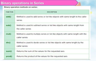
Binary operations inSeries
We can perform binary operation on series like addition,
subtraction and many other operation.
In order to perform binary operation on series we have to
use some function like .add(),.sub() etc..
Any item for which one or the other does not have an entry
is marked by NaN, or “Not a Number”, which is how Pandas
marks missing data.
40.
Binary operations inSeries
>>> import numpy as np
>>> s = pd.Series([1,2,3,4,np.NaN,5,np.NaN])
>>> s
0 1.0
1 2.0
2 3.0
3 4.0
4 NaN
5 5.0
6 NaN
dtype: float64
41.
Write a Pandasprogram to add, subtract, multiply and divide
two Pandas Series.
Program
import pandas as pd
ds1 = pd.Series([2, 4, 6, 8, 10])
ds2 = pd.Series([1, 3, 5, 7, 9])
ds = ds1 + ds2
print(“Sum of Series: n “ , ds)
ds = ds1 - ds2
print(“Subtraction of Series: n “ , ds)
ds = ds1 * ds2
print(“Product of two Series: n “, ds)
ds = ds1 / ds2
print(“Quotient of the Series: n “ , ds)
# importing pandasmodule
import pandas as pd
# creating a series
data = pd.Series([5, 2, 3,7], index=['a', 'b', 'c', 'd'])
# creating a series
data1 = pd.Series([1, 6, 4, 9], index=['a', 'b', 'd', 'e’])
# add two series using .add() function.
data.add(data1)
Program
44.
Write a Pandasprogram to compare the elements of the two
Pandas Series.
Program
import pandas as pd
ds1 = pd.Series([2, 4, 6, 8, 10])
ds2 = pd.Series([1, 3, 5, 7, 10])
print("Compare the elements of the said Series:")
print("Equals:")
print(ds1 == ds2)
print("Greater than:")
print(ds1 > ds2)
print("Less than:")
print(ds1 < ds2)
45.
Program – Tosort values
abc=pd.Series(['M','A','N','G','O','E','S'],index=[10,20,30,
40,50,60,70])
abc.sort_values()
abc.sort_index()
>>> abc
20 A
60 E
40 G
10 M
30 N
50 O
70 S
dtype: object
46.
Create series fromndarray
An array of values can be passed to a Series.
If data is an ndarray, index must be the same
length as data.
If no index is passed, one will be created having
values [0, ..., len(data) - 1].
47.
Create series fromndarray
import pandas as pd
import numpy as np
data = np.array(['a','b','c','d'])
s = pd.Series(data)
print (s)
Its output is as follows −
0 a
1 b
2 c
3 d
dtype: object
Note- We did not pass any index, so by default, it assigned the indexes ranging
from 0 to len(data)-1, i.e., 0 to 3.
48.
Create series fromndarray
import pandas as pd
import numpy as np
abc = np.array(['a','b','c','d'])
s = pd.Series(abc , index=[100,101,102,103])
print (s)
Its output is as follows −
100 a
101 b
102 c
103 d
dtype: object
We passed the index values here. Now we can see the customized indexed
values in the output.
49.
# To add5 marks to each student in the series
#creating a series from array and specified index
import pandas as pd
import numpy as np
Marks=np.array([455,478,477,405])
M1=pd.Series(Marks, index=[“Annie", “Resmi", "Sana", “Haya"])
print(M1)
for i, j in M1.items( ): # i – index , j - values
M1.at[i] = j+5 #increase each values
print (M1)
#at - Access a single value for a row/column label pair.
Program – Mathematical operations
50.
import pandas aspd
import numpy as np
a=np.random.randn(5)
>>> a
array([-0.63206378, -0.19692941, 0.3883878 , 0.35998536, 0.1873882 ])
>>> b=pandas.Series(a)
>>> b
0 -0.632064
1 -0.196929
2 0.388388
3 0.359985
4 0.187388
dtype: float64
numpy.random.randn()
Returns an array of defined shape, filled with random floating-point
samples.
Program – random.randn
51.
• A dictionarycan be passed as input to a Series.
• Dictionary keys are used to construct index.
d = {‘a': 1, ‘b': 0, 'c': 2}
a=pd.Series(d)
print(a)
Output-
a 1
b 0
c 2
dtype: int64
Create a Series from dictionary
52.
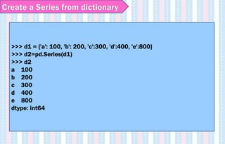
>>> d1 ={'a': 100, 'b': 200, 'c':300, 'd':400, 'e':800}
>>> d2=pd.Series(d1)
>>> d2
a 100
b 200
c 300
d 400
e 800
dtype: int64
Create a Series from dictionary
53.
>>> d3=pd.Series(d1,index=[20,30,40,50,60])
>>> d3
20NaN
30 NaN
40 NaN
50 NaN
60 NaN
dtype: float64
>>> d4=pd.Series(d1,index=['b','a','c','e','d'])
>>> d4
b 200
a 100
c 300
e 800
d 400
dtype: int64
Create a Series from dictionary
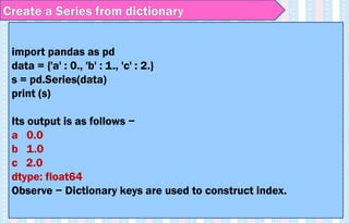
54.
import pandas aspd
data = {'a' : 0., 'b' : 1., 'c' : 2.}
s = pd.Series(data)
print (s)
Its output is as follows −
a 0.0
b 1.0
c 2.0
dtype: float64
Observe − Dictionary keys are used to construct index.
Create a Series from dictionary
55.
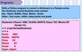
Programs-
Write a Pythonprogram to convert a dictionary to a Pandas series.
The dictionary named Students must contain-
Key : Name, RollNo, Class ,Marks , Grade
Value : Your name, rollNo, class,marks and grade
Students={'Name':‘ABC','RollNo':80978,'Class':'XII','Marks':87
,'Grade':'A'}
>>> s=pd.Series(Students)
>>> s
Name ABC
RollNo 80978
Class XII
Marks 87
Grade A
dtype: object
56.
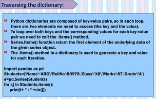
Traversing the dictionary:
Pythondictionaries are composed of key-value pairs, so in each loop,
there are two elements we need to access (the key and the value).
To loop over both keys and the corresponding values for each key-value
pair we need to call the .items() method.
Series.items() function return the first element of the underlying data of
the given series object.
The .items() method in a dictionary is used to generate a key and value
for each iteration.
import pandas as pd
Students={'Name':‘ABC','RollNo':80978,'Class':'XII','Marks':87,'Grade':'A'}
s=pd.Series(Students)
for i,j in Students.items():
print(i+ " : " +str(j))
57.
>>> pers ={'color': 'blue', 'fruit': 'apple', 'pet': 'dog'}
>>> p = pers.items()
>>> p # Here d_items is a view of items
dict_items([('color', 'blue'), ('fruit', 'apple'), ('pet', 'dog')])
>>> for item in pers.items():
print(item)
('color', 'blue')
('fruit', 'apple')
('pet', 'dog')
Traversing a dictionary
58.
for a,b inpers.items():
print(key, '->', value)
color -> blue
fruit -> apple
pet -> dog
ab ={"brand": "Ford", "model": "Mustang", "year": 1964}
for x, y in ab.items():
print(x, y)
brand Ford
model Mustang
year 1964
Traversing a dictionary
59.
Eg. Consider theseries created with names of students as index
and Marks as data using dictionary
import pandas as pd
d1={"Raj":234,"Gilbert":345}
m1=pd.Series(d1)
print(m1)
for i,j in m1.items():
m1.at[ i ]=j+5
print(m1)
Mathematical operations on Series
60.
When a scalaris passed, all the elements of the series is
initialized to the same value.
The value will be repeated to match the length of index.
import pandas as pd
s = pd.Series(5, index=[0, 1, 2, 3])
s
Its output is as follows −
0 5
1 5
2 5
3 5
dtype: int64
Create a Series from Scalar
61.
Create a serieswith scalar value 7 and index as ‘A’,’B’,’C’,’D’
s = pd.Series(7, index=['A','B','C','D'])
>>> s
A 7
B 7
C 7
D 7
dtype: int64
Create a Series from Scalar
62.
Create a Seriesusing string as index
ab = pd.Series(‘Welcome to India’, index=['A','B','C','D'])
>>> s
A Welcome to India
B Welcome to India
C Welcome to India
D Welcome to India
dtype: object
63.
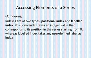
Accessing Elements ofa Series
(A)Indexing
Indexes are of two types: positional index and labelled
index. Positional index takes an integer value that
corresponds to its position in the series starting from 0,
whereas labelled index takes any user-defined label as
index
64.
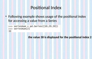
Positional Index
• Followingexample shows usage of the positional index
for accessing a value from a Series
the value 30 is displayed for the positional index 2
65.
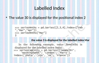
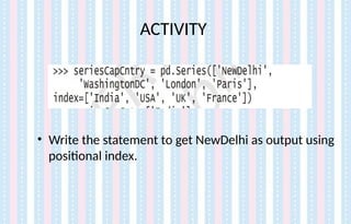
• More thanone element of a series can be accessed using a
list of positional integers or a list of index labels as shown in
the following examples:
>>> seriesCapCntry = pd.Series(['NewDelhi', 'WashingtonDC',
'London', 'Paris'], index=['India', 'USA', 'UK', 'France'])
>>> seriesCapCntry[[3,2]]
France Paris
UK London
dtype: object
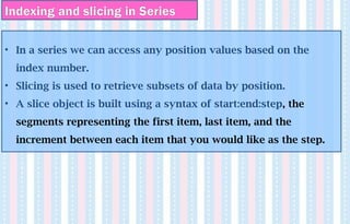
Indexing and slicingin Series
• In a series we can access any position values based on the
index number.
• Slicing is used to retrieve subsets of data by position.
• A slice object is built using a syntax of start:end:step, the
segments representing the first item, last item, and the
increment between each item that you would like as the step.
70.
Accessing Data fromSeries with indexing and slicing
import pandas aspd1
s = pd1.Series([1,2,3,4,5],index = ['a','b','c','d','e'])
>>> s[0]
1
>>> s[:3]
a 1
b 2
c 3
dtype: int64
>>> s[-3:]
c 3
d 4
e 5
dtype: int64
71.
>>> fruits =['apples', 'oranges', 'cherries', 'pears']
>>> S = pd.Series([20, 33, 52, 10], index=fruits)
>>> S
apples 20
oranges 33
cherries 52
pears 10
dtype: int64
>>> S['apples']
20
>>> S[0]
20
Accessing Data from Series with indexing and slicing
72.
Find out thefollowing-
AB
AB[2:4]
AB[1:6:2]
AB[ :6]
AB[4:]
AB[:4:2]
AB[4::2]
AB[::-1]
>>> num=[000,100,200,300,400,500,600,700,800,900]
>>> idx=['A','B','C','D','E','F','G','H','I','J']
>>> AB=pd.Series(num,index=idx)
Accessing Data from Series with indexing and slicing
73.
Find out thefollowing-
AB
AB[2:4]
AB[1:6:2]
AB[ :6]
AB[4:]
AB[:4:2] 0:4:2-- 000 200
AB[4::2] 400 600 800
AB[::-1]
>>> num=[000,100,200,300,400,500,600,700,800,900]
>>> idx=['A','B','C','D','E','F','G','H','I','J']
>>> AB=pd.Series(num,index=idx)
Accessing Data from Series with indexing and slicing
74.
Create a seriesusing 2 different lists
>>> import pandas as pd
>>> m=['jan','feb']
>>> n=[23,34]
>>> s=pd.Series(m,index=n)
>>> s
23 jan
34 feb
dtype: object
75.
Printing the sliceswith the values of the label index
>>> M = pd.Series([400,500,345,450],index=['Amit','Raj','Kris','Shon'])
>>> M
Amit 400
Raj 500
Kris 345
Shon 450
dtype: int64
>>> M['Kris']
345
M[['Raj','Kris','Shon']]
Raj 500
Kris 345
Shon 450
dtype: int64
M['Raj':'Shon']
Raj 500
Kris 345
Shon 450
dtype: int64
76.
Displaying the datausing Boolean indexing
# Eg. To select marks more than 400
>>> M = pd.Series([400,500,345,450],index=['Amit','Raj','Kris','Shon'])
>>> M
Amit 400
Raj 500
Kris 345
Shon 450
dtype: int64
>>> M>400
Amit False
Raj True
Kris False
Shon True
dtype: bool
>>> M[M>400] #Will display the names of students who got marks >400
Raj 500
Shon 450
dtype: int64
77.
Using range() tospecify index in series
>>> S=pd.Series(5,index=range(4))
>>> S
0 5
1 5
2 5
3 5
dtype: int64
>>> S=pd.Series([1,2,3,4],index=range(4))
>>> S
0 1
1 2
2 3
3 4
dtype: int64
78.
Using range() tospecify index in series –for loop
>>> S=pd.Series(range(1,15,3),index=[x for i in ‘abcde’])
>>> S
a 1
b 4
c 7
d 10
e 13
dtype: int64
>>> S=pd.Series([1,2,3,4.0],index=range(4))
>>> S
0 1.0
1 2.0
2 3.0
3 4.0
dtype: float64
79.
NaN - Creatinga series using missing values
In certain situations, we need to create a series object for which size is defined but
some element or datas are missing. This is handled by defining NaN(Not a Number )
values, which is an attribute of Numpy library.
This can be achieved by defining a missing value using np.Nan
80.
NaN - Creatinga series using missing values
Import pandas as pd
Import numpy as np
data = pd.Series([1, np.nan, 2, None, 3],
index= ('abcde'))
>>> data
a 1.0
b NaN
c 2.0
d NaN
e 3.0
dtype: float64
>>> d3=pd.Series(d1,index=[20,30,40,50,60])
>>> d3
20 NaN
30 NaN
40 NaN
50 NaN
60 NaN
dtype: float64
>>> s = pd.Series(np.nan, index=[49,3, 4, 5])
>>> s
49 NaN
3 NaN
4 NaN
5 NaN
dtype: float64
81.
Program
Write a pythonprogram to create a series of odd numbers.
odd=pd.Series(range(1, 10, 2))
>>> odd
0 1
1 3
2 5
3 7
4 9
dtype: int64
82.
Program
Create a serieswith names of any 7 colours :
• Display the first element
• Display the third element
• Display the first 3 elements (Using Slicing)
• Display the element starting from 2nd till 3rd (Using
Slicing)
• Display last 2 elements (Using Slicing)
83.
CREATING SERIES WITHRANGE AND FOR LOOP
>>> S=pd.Series(range(1,15,3),index=[x for x in 'abcde'])
>>> S
a 1
b 4
c 7
d 10
e 13
dtype: int64
84.
Handling floating pointvalues to generate a series
import pandas as pd
ab=pd.Series([2,4,6,7.5])
ab
0 2.0
1 4.0
2 6.0
3 7.5
Dtype : float64
Since 7.5 is a float value, it will convert the rest of the integer
values to float and so it be overall a float series.
85.
Indexing and accessingcan also be done using iloc and loc.
iloc- It is used for indexing or selecting based on position ie..
By row number and column number. It refers to position
based indexing.
Syntax is-
iloc=[<row number range>,<col number range>]
loc – It is used to index or select based on name ie.. By row
name and col name. It refers to name based indexing.
Syntax is-
loc=[<list of row name>,<list of col name>]
So, we can filter the data using the loc function in Pandas even
if the indices are not an integer in our dataset.
Note- By default, index is assigned from 0 to len-1.
iloc and loc
86.
import pandas aspd
a=pd.Series([1,2,3,4,5], index=‘a’,’b’,’c’,’d’,’e’])
>>> a.iloc[1:4] # Displays data using index
b 2
c 3
d 4
dtype: int64
>>> a.loc['b':'e'] # Displays data location wise
b 2
c 3
d 4
e 5
dtype: int64
loc and iloc
87.
>>> s =pd.Series(np.nan, index=[49,48,47,46,45, 1, 2, 3, 4, 5])
>>> s.iloc[:3] # slice the first three rows
49 NaN
48 NaN
47 NaN
>>> s.loc[:3] # slice up to and including label 3
49 NaN
48 NaN
47 NaN
46 NaN
45 NaN
1 NaN
2 NaN
3 NaN
loc and iloc
88.
loc vs. ilocin Pandas
loc
• Purely label-location based indexer for selection by label.
• It is primarily label based, but may also be used with a
boolean array.
• Allowed inputs are:
A single label, e.g. 5 or 'a'.
A list or array of labels, e.g. ['a', 'b', 'c'].
A slice object with labels, e.g. 'a':'f' (note that contrary to usual
python slices, both the start and the stop are included!).
A boolean array.
A callable function with one argument (the calling Series,
DataFrame ) and that returns valid output for indexing (one of
the above)
• Note : .loc will raise a KeyError when the items are not
found
89.
iloc-
• .iloc isprimarily integer position based (from 0 to length-
1 of the axis), but may also be used with a boolean array.
• .iloc will raise IndexError if a requested indexer is out-of-
bounds, except slice indexers which allow out-of-bounds
indexing.
• Allowed inputs are:
An integer e.g. 5
A list or array of integers [4, 3, 0]
A slice object with ints 1:7
A boolean array
A callable function with one argument
loc vs. iloc in Pandas
90.
It is atwo-dimensional data structure, just like any table (with
rows & columns).
Basic Features of DataFrame
Columns may be of different types
Size can be changed (Mutable)
Labelled axes (rows / columns)
Can perform arithmetic operations on rows and columns
CreateDataFrame
It can be created with the following-
Lists , dict , Series , Numpy arrays , Another DataFrame
Dataframes
91.
Structure of aDataframe
Pandas DataFrame consists of three principal components,
the data, rows, and columns.
You can think of it as an SQL table or a spreadsheet data representation.
92.
Dataframe Creation
Dataframes canbe created using constructor in pandas.
Syntax: pd.DataFrame( data, index, columns, dtype, copy)
Sr.No Parameter & Description
1 data - data takes various forms like ndarray, series, map, lists, dict,
constants and also another DataFrame.
2 index - For the row labels, the Index to be used for the resulting frame
is Optional Default np.arange(n) if no index is passed.
3 columns- For column labels, the optional default syntax is -
np.arange(n). This is only true if no index is passed.
4 dtype - Data type of each column.
5 copy - This command (or whatever it is) is used for copying of data, if
the default is False.
93.
Creating an emptyDataframe
A basic DataFrame, which can be created is an Empty Dataframe.
>>> import pandas as pd
>>> d=pd.DataFrame()
>>> d
Empty DataFrame
Columns: []
Index: []
94.
Series vs Dataframe
ASeries is essentially a column, and a DataFrame is a multi-dimensional
table made up of a collection of Series.
95.
Creating a Dataframefrom lists with values only
The DataFrame can be created using a single list or a list of lists.
CREATING A DATAFRAME FROM SINGLE LIST
Example1:
import pandas as pd
data = [1,2,3,4,5]
df = pd.DataFrame(data)
print (df)
96.
Creating a Dataframefrom lists of lists (multidimensional list)
CREATE A DATAFRAME FROM A LIST OF LISTS
import pandas as pd
data = [['Alex',10],['Bob',12],['Clarke',13]]
df = pd.DataFrame(data,columns=['Name','Age'])
print (df)
Name Age
0 Alex 10
1 Bob 12
2 Clarke 13
97.
Creating a Dataframefrom lists of lists (multidimensional list)
import pandas as pd
>>> a=[12,13,14,15]
>>> b=[20,30,40,50]
>>> c=pd.DataFrame(a,index=[b],columns=['Numbers'],dtype='float')
>>> c
Numbers
20 12.0
30 13.0
40 14.0
50 15.0
Creating a Dataframefrom lists of lists (multidimensional list)
Using multi-dimensional list with column name and dtype
specified.
import pandas as pd
lst = [['tom', 'reacher', 25], ['krish', 'pete', 30],
['nick', 'wilson', 26], ['juli', 'williams', 22]]
df = pd.DataFrame(lst, columns =['FName', 'LName', 'Age'],
dtype = float)
df
100.
Program
Display the followingdetails in a dataframe.
Name Marks Index
Vijaya 80 B1
Rahul 92 A2
Meghna 67 C
Radhika 95 A1
Shaurya 97 A1
df = pd.DataFrame(lst, columns =['FName', 'LName', 'Age'], dtype = float)
Creating DataFrames fromSeries
DataFrames are 2 dimensional representation of Series.
When we represent 2 or more series in the form of rows and columns,
it becomes a dataframe.
Lets create 2 series and pass it into a dataframe.
>>> p={'one':pd.Series([1,2,3], index=['a','b','c']), 'two':pd.Series
([11,22,33,44], index=['a','b','c','d'])}
>>> q=pd.DataFrame(p)
>>> q
one two
a 1.0 11
b 2.0 22
c 3.0 33
d NaN 44
Creating DataFrames fromSeries
# To create dataframe from 2 series of student data
import pandas as pd
stud_marks=pd.Series([89,94,93,83,89],index=['Anuj','Deepak','Sohail'
,'Tresa','Hima'])
stud_age=pd.Series([18,17,19,16,18],index=['Anuj','Deepak','Sohail','Tre
sa','Hima'])
>>> stud=pd.DataFrame({'Marks':stud_marks,'Age':stud_age})
>>> stud
Marks Age
Anuj 89 18
Deepak 94 17
Sohail 93 19
Tresa 83 16
Hima 89 18
105.
Sorting data inDataFrames
We can sort the data inside a dataframe using sort_values().
Here 2 arguments are passed- sorting field and the order of sorting (asc
or desc).
‘By’ keyword, defines the name of the field or column based on which
it is to be sorted.
>>> stud.sort_values(by=['Marks'])
Marks Age
Tresa 83 16
Anuj 89 18
Hima 89 18
Sohail 93 19
Deepak 94 17
stud.sort_values(by=['Marks'],ascending=False)
Marks Age
Deepak 94 17
Sohail 93 19
Anuj 89 18
Hima 89 18
Tresa 83 16
106.
Creating DataFrame fromDictionary (Dictionary of Lists)
• List of dictionaries can be passed as an input data to create a dataframe.
• The dictionary keys are by default, taken as column names.
import pandas as pd
data = {'Name':['Tom', 'Jack', 'Steve', 'Ricky'],'Age':[28,34,29,42]}
df = pd.DataFrame(data)
print (df)
Age Name
0 28 Tom
1 34 Jack
2 29 Steve
3 42 Ricky
107.
Program
cars = {'Brand':['Honda Civic','Toyota Corolla','Ford Focus','Audi A4'],
'Price': [22000,25000,27000,35000] }
df = pd.DataFrame(cars, columns = ['Brand', 'Price'])
print (df)
Brand Price
0 Honda Civic 22000
1 Toyota Corolla 25000
2 Ford Focus 27000
3 Audi A4 35000
Brand Price
car1 Honda Civic 22000
car2 Toyota Corolla 25000
car3 Ford Focus 27000
car4 Audi A4 35000
108.
import pandas aspd
data = { ‘Name ‘ : [ ‘Tom’,’Jack’,’Steve’,’Ricky’], ‘Age’ : [28,34,29,42] }
df = pd.DataFrame (data, index = [‘rank 1’, ‘rank 2’, ‘rank 3’, ‘rank 4’ ])
print ( df )
output
AGE NAME
RANK 1 28 tOM
RANK 2 34 jACK
RANK 3 29 Steve
RANK 4 42 Ricky
Program - Create an indexed DataFrame
109.
Create a programthat shows the month and number of days in a
month.
Day Month
0 31 Jan
1 30 Apr
2 31 Mar
3 30 June
Program
110.
DataFrame.set_index (<ColumnName>, inplace=True)
–This method selects the column specified as the row index
DataFrame.reset_index(inplace=True)
- The method will reset the row index to the default index as
0,1,2,3… etc.
Setting a column of dataframe as row index & resetting to
default row index
111.
Suppose we wantto make one of the columns as row index:
import pandas as pd
data = {'Name':['Tom', 'Jack', 'Steve', 'Ricky'],'Age':[28,34,29,42]}
df = pd.DataFrame(data)
df.set_index('Name',inplace=True)
print (df)
Age
Name
Tom 28
Jack 34
Steve 29
Ricky 42
Example
112.
CREATE A DATAFRAMEFROM DICTIONARY OF LIST TO DISPLAY THE
FOLLOWING OUPUT
Program
Events Ruby Emerald Sapphire
Cat_1 Skipping 30 20 20
Cat_2 BasketBall 40 30 20
Cat_3 Running 40 20 30
113.
# Create aDataFrame from List of Dictionaries
import pandas as pd
data1 = [{'x': 1, 'y': 2},{'x': 5, 'y': 4, 'z':5}]
df1 =pd.DataFrame(data1)
x y z
0 1 2 NaN
1 5 4 5.0
Note − Observe, NaN (Not a Number) is appended in missing
areas.
Program
114.
Create a DataFramewith a list of dictionaries, row indices, and
column indices.
import pandas as pd
data = [{'a': 1, 'b': 2},{'a': 5, 'b': 10, 'c': 20}]
df1 = pd.DataFrame(data, index=['first', 'second'], columns=['a',
'b‘,’c’])
>>> df1
a b c
first 1 2 NaN
second 5 10 20.0
Program
115.
Create aseries from a one list containing authors name and another list
containing number of articles written.
Create a dataframe from the series created using a dictionary containing key as
“Authors” and “Articles”
The following output must be obtained:
Program
import pandas as pd
a=["Jitender","Purnima","Arpit","Jyoti"]
b=[210,211,114,178]
s = pd.Series(a)
s1= pd.Series(b)
df=pd.DataFrame({"Author":s,"Article":s1})
df
116.
• To accessand retrieve the records from a dataframe, we need to use slice
operation.
• Slicing will display the retrieved records as per the defined range.
import pandas as pd
student={'Name':['Rinku','Ritu','Ajay','Pankaj','Aditya'], 'English':[84,56,89,
78,36], 'Economics':[96,56,89,45,95], 'IP':[83,85,88,92,97], 'Accounts':
[77,75,63,89,85]}
>>> df=pd.DataFrame(student)
>>> df
Name English Economics IP Accounts
0 Rinku 84 96 83 77
1 Ritu 56 56 85 75
2 Ajay 89 89 88 63
3 Pankaj 78 45 92 89
4 Aditya 36 95 97 85
Selecting & Accessing from DataFrame
117.
df[1:4] # Recordsfrom 1st
to 3rd
row are displayed
Name English Economics IP Accounts
1 Ritu 56 56 85 75
2 Ajay 89 89 88 63
3 Pankaj 78 45 92 89
Note- Single row accessing is not possible.
To display a whole column,
>>> df['Name']
To display more than 1 columns,
>>> df[['Name','IP']]
>>> df['Name'][0:3]
0 Rinku
1 Ritu
2 Ajay
Name: Name, dtype: object
Selecting & Accessing from DataFrame
118.
• Pandas providesus the flexibility to even change or rename any column inside a
dataframe.
• To change for a single column-
df.rename(columns={'Name':'Emp_Name'}, inplace=True)
• Consider a list of age of students-
a1=[20,30,25,26,15]
Rename the column ‘a1’ to ‘age’
>>> a1=[20,30,25,26,15]
>>> a1
[20, 30, 25, 26, 15]
Renaming column in DataFrame
>>> df=pd.DataFrame(a1)
>>> df
0
0 20
1 30
2 25
3 26
4 15
>>> df.columns=['Age']
>>> df
Age
0 20
1 30
2 25
3 26
4 15
119.
• To addnew columns to an already existing dataframe, the syntax is-
dfobject.colname[row_label]=new_value
>>> df['Age1']=45 # the entire column is filled up with 45
>>> df
Age Age1
0 20 45
1 30 45
2 25 45
3 26 45
4 15 45
Adding column to a DataFrame
df['Age3']=pd.Series([42,35,44,50,60])
df
Age Age2 Age3
0 20 45 42
1 30 45 35
2 25 45 44
3 26 45 50
4 15 45 60
df['Total']=df['Age']+df['Age2']+df['Age3']
df
Age Age2 Age3 Total
0 20 45 42 107
1 30 45 35 110
2 25 45 44 114
3 26 45 50 121
4 15 45 60 120
120.
• We canupdate a column values by using arithmetic operators.
• We can also assign or copy the values of a dataframe with the help of assignment
operator.
• To add a new column for updated_age after 10 years for all students,
>>> df['Total']=df['Total']+10
>>> df
Age Age2 Age3 Total
0 20 45 42 117
1 30 45 35 120
2 25 45 44 124
3 26 45 50 131
4 15 45 60 130
>>> df['Updated_Age']=df['Total']
>>> df
Age Age2 Age3 Total Updated_Age
0 20 45 42 117 117
1 30 45 35 120 120
2 25 45 44 124 124
3 26 45 50 131 131
4 15 45 60 130 130
Adding column to a DataFrame
121.
1. Create adataframe from the dictionary of list.
Name Height Qualification
0 Jai 5.1 Msc
1 Princi 6.2 MA
2 Gaurav 5.1 Msc
3 Anuj 5.2 Msc
2. Add a column address to the dataframe with values:
address = ['Delhi', 'Bangalore', 'Chennai', 'Patna']
Sample Question-
122.
data = {'Name':['Jai', 'Princi', 'Gaurav', 'Anuj'],'Height': [5.1, 6.2, 5.1,
5.2],'Qualification': ['Msc', 'MA', 'Msc', 'Msc']}
df = pd.DataFrame(data)
>>> df['address']=['Delhi', 'Bangalore', 'Chennai', 'Patna']
>>> df
Name Height Qualification address
0 Jai 5.1 Msc Delhi
1 Princi 6.2 MA Bangalore
2 Gaurav 5.1 Msc Chennai
3 Anuj 5.2 Msc Patna
Sample Question-
123.
Based on thegiven table, students are asked to create a dataframe
from a dictionary of list and perform the following:
• Change the name of the column ‘Marks’ as ‘Eng_Marks’
• Add another column ‘IP_Marks’ with a series of values
(56,78,89,77,99)
• Create a column ‘ TotalMarks’ which stores the total of Eng & IP
marks
• Display the dataframe with all the columns
Sample Question-
Name Subject Marks
0 Rahul Math 75
1 Sahil Science 80
2 Muskan Computer 69
3 Aryan SST 94
4 Vansh English 79
124.
• DataFrame.index- Theindex (row labels) of the DataFrame.If the row
index has default values then RangeIndex(start=0, stop=4, step=1) is
displayed
• DataFrame.columns- Returns the column names/ column index with
dtype
• DataFrame.dtypes- Return the data types of column in the DataFrame
and also the datatype of the DataFrame.
• DataFrame.size - Return an int representing the number of elements in
the Dataframe object.
• DataFrame.shape- Return a tuple representing the dimensionality of
the DataFrame ie., the number of rows and columns in the dataframe
Properties of DataFrame-
125.
>>>df
Name Height Qualificationaddress
0 Jai 5.1 Msc Delhi
1 Princi 6.2 MA Bangalore
2 Gaurav 5.1 Msc Chennai
3 Anuj 5.2 Msc Patna
>>> df.size
16
>>> df.shape
(4, 4)
>>> df.dtypes
Name object
Height float64
Qualification object
address object
dtype: object
Properties of DataFrame-
126.
What will thefollowing fuctions return:
a) df.columns
b)df.index
c)df.shape
d)df.size
Sample Question-
• The methodof selecting / accessing a column of a dataframe is
similar to slicing using series.
• Pandas provides 3 methods to access dataframe column(s)
Using the format of square brackets followed by the name of the
column passed as a string value, like
df_object.[‘column_name’]
Using the dot notation df_object.column_name
Using numeric indexing and the iloc attribute, like
df_object.iloc[:,<column_number>]
• Here , i stands for integer, which signifies that this command shall
return a numeric value denoting the row and column range
SELECTING A COLUMN FROM A DATAFRAME
Consider the dataframeas shown:
• DataFrame has two ordered axis.
• One goes across the top, the other goes down the left side.
The index value: This is what you will see when you visualize a DataFrame
(The bolded black values on the vertical and horizontal axis below)
The index position: This does not get visualized and simply represents the
ordering of the rows or columns.
USING iLOC TO RETRIEVE COLUMNS
131.
USING iLOC TORETRIEVE COLUMNS
Vertical Index Values: [0, 1, 2, 3, 4]
Vertical Index Positions: [0, 1, 2, 3, 4]
Horizontal Index Values: [‘fruit_name’, ‘price, ‘color’, ‘sweetness’]
Horizontal Index Positions: [0, 1, 2, 3]
132.
USING iLOC TORETRIEVE COLUMNS
iloc allows us to index a DataFrame in the same way that we
can index a list; based on index position.
The difference is that a DataFrame has a two-dimensional
index, so we need to pass in slicers for the rows first and
then for the columns.
There are four 4 possible types of slicers we can use on the
table given:
• Scalar positions (eg:- 0,3,4)
• Range of positions (eg:- 0:1, 1:4)
• All positions (:)
• List of positions (eg:- [0,3] , [1,5])
133.
If we wantto select the data in row 2 and column 0 (i.e., row
index 2 and column index 0) we’ll use the following code:
df.iloc[2,0]
USING iloc- Integer locate
USING iloc- Integerlocate
• When we “slice” our data, we take multiple rows or multiple columns
• Keep in mind that the row number specified by the stop index value
is not included.
138.
Example - USINGiloc- Integer locate
>>> df
>>> df
Date Event Cost
0 10/2/2011 Music 10000
1 11/2/2011 Poetry 5000
2 12/2/2011 Theatre 15000
3 13/2/11 Comedy 2000
>>> df.iloc[:,:]
Date Event Cost
0 10/2/2011 Music 10000
1 11/2/2011 Poetry 5000
2 12/2/2011 Theatre 15000
3 13/2/11 Comedy 2000
>>> df.iloc[:,0:2]
Date Event
0 10/2/2011 Music
1 11/2/2011 Poetry
2 12/2/2011 Theatre
3 13/2/11 Comedy
>>> df.iloc[0:2,:]
Date Event Cost
0 10/2/2011 Music 10000
1 11/2/2011 Poetry 5000
139.
USING iloc- Integerlocate
>>> df
Date Event Cost
0 10/2/2011 Music 10000
1 11/2/2011 Poetry 5000
2 12/2/2011 Theatre 15000
3 13/2/11 Comedy 2000
>>> df.iloc[[0,3],[0,1]]
Date Event
0 10/2/2011 Music
4 13/2/11 Comedy
>>> df.iloc[[0,3],[0,2]]
Date Cost
0 10/2/2011 10000
3 13/2/11 2000
140.
USING iloc- Integerlocate
To display only columns Date and Cost,
>>> df[['Date','Cost']]
Date Cost
0 10/2/2011 10000
1 11/2/2011 5000
2 12/2/2011 15000
3 13/2/11 2000
>>> df.iloc[:,[0,2]]
Date Cost
0 10/2/2011 10000
1 11/2/2011 5000
2 12/2/2011 15000
3 13/2/11 2000
DELETING A COLUMNOR ROW FROM A DATAFRAME
• Using del keyword
• Using pop method
• Using drop method
143.
DELETING A COLUMNFROM A DATAFRAME
• Using del keyword – [ONLY FOR COLUMN , 1 column at a time]
del df[‘<column name>’]
This will only delete the particular column , after which we have to display the
dataframe to see the changes.
>>> del df['Date']
>>> df
Event Cost
0 Music 10000
1 Poetry 5000
2 Theatre 15000
3 Comedy 2000
144.
DELETING A COLUMNFROM A DATAFRAME
• Using pop method –
df.pop(‘<Column Name>’)-
It deletes and will display the column name that is removed from the dataframe.
>>> df.pop('Cost')
0 10000
1 5000
2 15000
3 2000
Name: Cost, dtype: int64
>>> df
Event
0 Music
1 Poetry
2 Theatre
3 Comedy
145.
DELETING A ROWOR COLUMN FROM A DATAFRAME
• Using drop method – drop (labels, axis=1)
It will return a new dataframe with the columns deleted. Axis=1 means column
and axis=0 means row. By default it is 0.
To remove any row,
>>> df.drop([0]) OR >>> df.drop([0],axis=0)
Date Event Cost
1 11/2/2011 Poetry 5000
2 12/2/2011 Theatre 15000
3 13/2/11 Comedy 2000
To remove any column,
>>> df.drop(['Date'],axis=1)
Event Cost
0 Music 10000
1 Poetry 5000
2 Theatre 15000
4 Comedy 2000
To remove a column permanently from your dataframe
you will need to provide one more parameter
inplace=True.
146.
DELETING A ROWOR COLUMN FROM A DATAFRAME
• To delete multiple columns :
df.drop([‘Column1’, ‘Column2’], axis=1, inplace = True)
OR
df.drop(columns=[‘Column1’, ‘Column2’], axis=1, inplace = True)
To drop rows :
df.drop([‘row1’,’row2’], axis= 0, inplace = True)
OR
df.drop(index=[‘row1’,’row2’], axis=0, inplace = True)
147.
DELETING A COLUMN- Practical Implementation
• Create a simple dataframe with a dictionary of lists, and column
names: name, year, orders, town.
• Remove the column orders from the dataframe using del df[]
• Remove the column ‘name’ using df.pop( )
• Remove the column town using df.drop ()
148.
Accessing elements usingloc
loc –
The loc() function is used to access a group of rows and columns
by label(s).
149.
Accessing elements usingloc
>>>df = pd.DataFrame({"A":[12, 4, 5, None, 1],"B":[7, 2, 54, 3, None],
"C":[20, 16, 11, 3, 8], "D":[14, 3, None, 2, 6]})
>>> df.iloc[0,2]
20
>>> df.loc[0,'B']
7.0
>>> >>> df.iloc[0:2,0:2]
A B
0 12.0 7.0
1 4.0 2.0
>>> df.loc[0:2,"A":"C"]
A B C
0 12.0 7.0 20
1 4.0 2.0 16
2 5.0 54.0 11
150.
Accessing elements usingloc
>>> df.iloc[:,0:2]
A B
0 12.0 7.0
1 4.0 2.0
2 5.0 54.0
3 NaN 3.0
4 1.0 NaN
>>> df.loc[:,"A":"C"]
A B C
0 12.0 7.0 20
1 4.0 2.0 16
2 5.0 54.0 11
3 NaN 3.0 3
4 1.0 NaN 8
>>> df.iloc[[1,3],[2,1]]
C B
1 16 2.0
3 3 3.0
>>> df.loc[[1,3],
["A","C"]]
A C
1 4.0 16
3 NaN 3
151.
Head and Tailin DataFrame
The method head() gives the first 5
rows and tail gives the last 5.
import pandas as pd
emp={'id':
[100,101,102,103,105,106,107],'na
me':
['Raj','Sini','Flora','Leena','Priya','De
nny','Kevin'],'Sal':
[12000,5000,2200,3200,23000,8700,
15000]}
df=pd.DataFrame(emp)
print(df)
print(df.head())
print(df.tail())
print(df.head(2))
print(df.tail(3))
id name Sal
0 100 Raj 12000
1 101 Sini 5000
2 102 Flora 2200
3 103 Leena 3200
4 105 Priya 23000
5 106 Denny 8700
6 107 Kevin 15000
id name Sal
0 100 Raj 12000
1 101 Sini 5000
2 102 Flora 2200
3 103 Leena 3200
4 105 Priya 23000
id name Sal
2 102 Flora 2200
3 103 Leena 3200
4 105 Priya 23000
5 106 Denny 8700
6 107 Kevin 15000
id name Sal
0 100 Raj 12000
7 101 Sini 5000
id name Sal
4 105 Priya 23000
5 106 Denny 8700
6 107 Kevin 15000
152.
Transpose
T:- Transpose thedataframe (row convert into columns & columns convert into
rows.
>>> x
month sales1 sales2
0 jan 5 3
1 feb 7 5
2 mar 6 8
>>> x.T
0 1 2
month jan feb mar
sales1 5 7 6
sales2 3 5 8
153.
reindex
Reindex will changethe order of index .
>>> x=pd.DataFrame({'month':['jan','feb','mar'], 'sales1':[5,7,6],'sales2':[3,5,8]})
>>> x
month sales1 sales2
0 jan 5 3
1 feb 7 5
2 mar 6 8
>>> y=x.reindex([2,1,0])
>>> y
month sales1 sales2
2 mar 6 8
1 feb 7 5
0 jan 5 3
154.
Binary operations
Pandas providesthe methods add(), sub(), mul(), div() for carrying out binary
operations on dataframes.
Since all these operations involve 2 dataframes to act upon, they are called
Binary. (‘bi’ means ‘two’ and ‘ary’ means digits)
>>> S1=pd.DataFrame({'UT-1':[23,20,21,19,25],'UT-2':[20,23,12,16,23]})
>>> S2=pd.DataFrame({'UT-1':[13,21,22,10,21],'UT-2':[24,23,11,12,24]})
>>> S1.add(S2)
UT-1 UT-2
0 36 44
1 41 46
2 43 23
3 29 28
4 46 47
1.Write the purposeof the following statement:
mtns_df.set_index('name', inplace=True)
2. Write the output of the statement:
a. mtns.loc[:, 'summited’]
b. mtns.loc['K2', :]
c. mtns.loc['K2', 'summited’]
d. mtns.loc[['K2', 'Lhotse'], :]
e. mtns.loc[:, 'height': 'summited’]
f. mtns.loc[mtns.loc[:, 'summited'] > 1954, :]
g. mtns.iloc[0, :]
h. mtns.iloc[:, 2]
i. mtns.iloc[0, 2]
j. mtns.iloc[[1, 3], :]
k. mtns.iloc[:, 0:2]
157.
Accessing a DataFramewith a boolean index
• We can create Boolean indexes for dataFrames and searching can be done
based on True or False indexes.
• loc() is used.
• Pandas, DataFrame also support Boolean indexing.
• So we can direct search our data based on True or False indexing.
• We can use loc[ ] for this purpose.
• In order to access a dataframe with a boolean index, we have to create a
dataframe in which index of dataframe contains a boolean value that is
“True” or “False”.
import pandas as pd
dict= {'name':[“Mohak", “Freya", “Roshni"], 'degree': ["MBA", "BCA", "M.Tech"],
'score':[90, 40, 80]}
df= pd.DataFrame(dict, index = [True, False, True])
print(df.loc[True])
158.
Accessing a DataFramewith a boolean index
import pandas as pd
data1={ 'rollno' : [101,102,103,104],
'name' : ['ram','mohan','sohan','rohan'] }
student1 = pd.DataFrame(data1,
index = [True, False, True, False],
columns=['rollno' , 'name']
)
print(student1)
Output rollno name
True 101 ram
False 102 mohan
True 103 sohan
False 104 rohan
print(student1.loc[True] )
Output rollno name
True 101 ram
True 103 sohan
-----------------------
print(student1.loc[False] )
Output rollno name
False 102 mohan
False 104 rohan
159.
Iteration on rowsand columns
• If we want to access row or column from a dataframe row or
column wise then iteration is used.
• Pandas provides 2 functions to perform iterations-
1. iterrows()
2. iteritems()
160.
iterrows
• It isused to access the data row wise.
import pandas as pd
ab= [{'Name':'Arya','Age':20},{'Name':'Shane','Age':19}]
df=pd.DataFrame(ab)
for(i,j) in df.iterrows():
print(j)
Name Arya
Age 20
Name: 0, dtype: object
Name Shane
Age 19
Name: 1, dtype: object
161.
iteritems
• It isused to access the data column wise.
import pandas as pd
ab= [{'Name':'Arya','Age':20},{'Name':'Shane','Age':19}]
df=pd.DataFrame(ab)
for(i,j) in df.iteritems():
print(j)
0 Arya
1 Shane
Name: Name, dtype: object
0 20
1 19
Name: Age, dtype: int64
Sorting data inDataFrames
sort_values() Seen earlier
sort_index() To sort by index
>>> student.sort_index()
rollno name
0 10.0 ram
1 NaN 110
2 103.0 sohan
3 104.0 rohan
>>> student.sort_index(ascending=False)
rollno name
3 104.0 rohan
2 103.0 sohan
1 NaN 110
0 10.0 ram
>>> student.sort_index(axis=1)
name rollno
0 ram 10.0
1 110 NaN
2 sohan 103.0
3 rohan 104.0
169.
Create DataFrame fromcsv
CSV (Comma Separated Values) is a simple file format used to
store tabular data, such as a spreadsheet or database.
A CSV file stores tabular data (numbers and text) in plain text.
Each line of the file is a data record.
Each record consists of one or more fields, separated by
commas.
The use of the comma as a field separator is the source of the
name for this file format.
170.
Create DataFrame fromcsv
For working with CSV files in Python, there is an in-built
module called csv.
Files of this format are generally used to exchange data,
usually when there is a large amount, between different
applications.
171.
Advantages of CSVformat
• A simple and compact format for data storage.
• A common format for data interchange.
• It can be opened in popular spreadsheet packages like MS
Excel, Open Office-Calc, etc.
• Nearly all spreadsheets and databases support import/export
to CSV format.
172.
Create DataFrame fromcsv
A CSV is a text file, so it can be created and edited using any
text editor.
A file is to be created and saved in the same folder where our
programs are saved.
To create a DataFrame from the file we need to first import
data from csvfile.
pd.read_csv( ) is the method, which is used to read csv file
from other location.
173.
Using MS excel
Let us create a CSV file using Microsoft Excel on the basis of
“Employee” table.
174.
Using MS excel
1.Launch Microsoft Excel.
2. Type the data given in the above Table in the Excel sheet .
You will also notice that some cell values are missing to represent missing
values (NaN) in Pandas dataframe.
175.
Using MS excel
3.Save the file with a proper name by clicking File -> Save or Save As or
press Ctrl + S to open the Save As window .
4. Type the name of the file as Employee and select file type as CSV
(Comma delimited) (*.csv) from the drop-down arrow.
5. Click on Save button. Excel will ask for confirmation to select CSV format.
6. Click on OK.
176.
Using MS excel
•Lastly, click on Yes to retain and save the Excel file in CSV format.
• To view this CSV file, open any Text Editor (Notepad preferably) and
explore the folder containing Employee.csv file.
• If you open the file in a Notepad editor, you will observe that each
column is separated by a comma (,) delimiter and each new line
indicates a new row/record.
177.
Open csv fileusing Pandas DataFrame
After creating a simple “Employee” CSV file, it can be read using read_csv()
function in Pandas once you know the path of your file.
The read_csv method loads the data in a Pandas dataframe ‘df’.
pd.read_csv(“path”) shall fetch the data from csv file and display all records
at the command prompt.
Syntax for read_csv() method is:
import pandas as pd
<df>=pd.read_csv(<FilePath>)
178.
Creating a csvfrom .txt file
Create a text file with comma separated values.
First entry being ‘the names of columns’
Example:
#Creating a dataframe from a text file
import pandas as pd
df=pd.read_csv("sample.txt")
print(df)
print (df.columns)
Unnamed: 0 column gets displayed automatically along with the
index values. To avoid this column, use the attribute index_col =0
with read_csv() method.
179.
More commands
• Todisplay the shape (number of rows and columns) of the CSV file
df.shape
>>> df.shape
(7, 5)
Reading CSV file with specific/selected columns-
• This can be done by using “usecols” attribute along with read_csv().
>>> df=pd.read_csv("Employee.csv",usecols=['Name','Age'])
Reading CSV file with specific/selected rows-
• Use “nrows” attribute used with read_csv(). nrows means number of
rows.
>>> df=pd.read_csv("Employee.csv",nrows=5)
• Here 5 rows are displayed. It will display NaN values also, if present.
180.
More commands
Reading CSVfile without header
• To avoid displaying the header of the dataframe, use
header=None option.
>>> df=pd.read_csv("Employee.csv",header=None)
Reading CSV file without index
• To avoid displaying index numbers, use index_col=0.
>>> df=pd.read_csv("Employee.csv",index_col=0)
181.
UPDATING/MODIFYING CONTENTS INA CSV FILE
Reading CSV file with new column names
• Use skiprow option to skip the header if it exists. Specify the new
names with names option.
df=pd.read_csv("Employee.csv",skiprows=1,names=['a','b','c','d','e'])
Replace any contents of the dataframe with NaN values-
• Done by using na_values option along with read_csv method
>>> df=pd.read_csv("Employee.csv",na_values=[26])
Here wherever the value 26 is seen, it gets updated to NaN.
182.
Exporting data fromDataFrame to csv
• To create a CSV file from a dataframe, the to_csv() method is
used.
• 2 methods-
Create a dataframe. Transfer this to a csv file.
Copying the contents of the original CSV file to another file.
• To export a dataframe into a csv file, 1st
create a dataframe say
df1 and use dataframe.to_csv(‘path’) method to export df1
into a new csv.
>>> df1=pd.DataFrame(df)
>>> df1.to_csv("Employee12.csv")
• Now the contents of df are copied to df1.
183.
Example
import pandas aspd
cars = {'Brand': ['Honda Civic','ToyotaCorolla',
'FordFocus','AudiA4'],'Price': [22000,25000,27000,35000]}
df= pd.DataFrame(cars, columns= ['Brand', 'Price'])
df.to_csv('export_dataframe.csv', index = False, header=True)
#Open the notepad with export_dataframe file.
pd.read_csv('export_dataframe.csv')
184.
Example
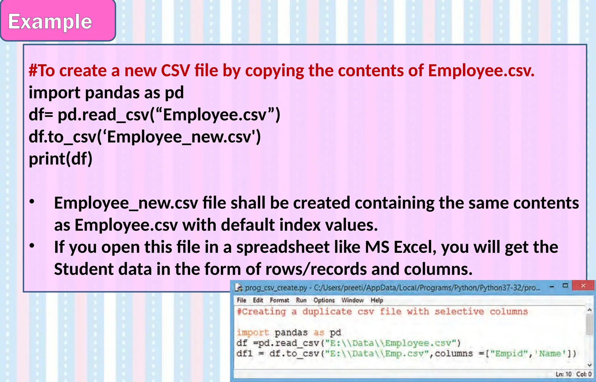
#To create anew CSV file by copying the contents of Employee.csv.
import pandas as pd
df= pd.read_csv(“Employee.csv”)
df.to_csv(‘Employee_new.csv')
print(df)
• Employee_new.csv file shall be created containing the same contents
as Employee.csv with default index values.
• If you open this file in a spreadsheet like MS Excel, you will get the
Student data in the form of rows/records and columns.


![Pandas Datatypes :
Pandas dtype Python Type NumPy type Usage
object Str String_, unicode_ Text
int64 Int int, int8, int16, int32,
int64, uint8, uint16,
uint32, uint64
Integer
numbers
float64 Float float, float16, float32,
float64
Floating point
numbers
bool bool bool True / False
datetime64 NA datetime64[ns] Date & Time
values](https://image.slidesharecdn.com/ln-250918173733-5ea4f2ca/85/Ln-1-Data-Handling-using-Pandas-I-1-pptx-14-320.jpg)
![A basic series, which can be created is an Empty Series.
Example - [Here ‘s’ is the Series Object]
import pandas as pd
s = pd.Series()
print s
Its output is as follows −
Series([], dtype: float64)
Note –
• Series () displays an empty list along with its default data type.
• Pd is an alternate name given to the Pandas module. Its significance is that we
can use ‘pd’ instead of typing Pandas every time we need to use it.
• Import statement is used for loading Pandas module into the memory and can
be used to work with.
Creation of Empty Series](https://image.slidesharecdn.com/ln-250918173733-5ea4f2ca/85/Ln-1-Data-Handling-using-Pandas-I-1-pptx-19-320.jpg)
![Creating DataSeries with a list
Syntax:
<Series Object>=pandas.Series([data],index=[index])
Eg:-
import pandas as pd
s=pd.Series( [ 2,4,6,8,10])
print(s)
S- is a series variable
Series() – method displays a list along with
default data type
pd is the alternative name given to panda
module
Import statement is used to load pandas
module into the memory and can be used](https://image.slidesharecdn.com/ln-250918173733-5ea4f2ca/85/Ln-1-Data-Handling-using-Pandas-I-1-pptx-20-320.jpg)
![Program- DataSeries
>>> s= pandas.Series ( [3,-5,7,4] , index=['a','b','c','d‘] )
>>> s
Output:
a 3
b -5
c 7
d 4
dtype: int64](https://image.slidesharecdn.com/ln-250918173733-5ea4f2ca/85/Ln-1-Data-Handling-using-Pandas-I-1-pptx-21-320.jpg)
![>>> st = pd.Series([20, 70, 10], index=['frog', 'fish', 'hawk'])
>>> st
frog 20
fish 70
hawk 10
dtype: int64
>>> st.index.name = 'Animals'
>>> st
Animals
frog 20
fish 70
hawk 10
dtype: int64
Program](https://image.slidesharecdn.com/ln-250918173733-5ea4f2ca/85/Ln-1-Data-Handling-using-Pandas-I-1-pptx-22-320.jpg)


![Program
Months=[‘Jan’,’Feb’,’Mar’,’Apr’,’June’, ‘July’]
import pandas as pd
S=pd.Series(Months)
>>> S
0 Jan
1 Feb
2 Mar
3 Apr
4 June
5 July
dtype: object](https://image.slidesharecdn.com/ln-250918173733-5ea4f2ca/85/Ln-1-Data-Handling-using-Pandas-I-1-pptx-25-320.jpg)
![Accessing Series index and values
#Index and values are attributes of Series.
>>> Months=['Jan','Feb','Mar','Apr','June', 'July']
>>> Months
['Jan', 'Feb', 'Mar', 'Apr', 'June', 'July']
>>> a=pd.Series(Months)
>>> a.index
RangeIndex(start=0, stop=6, step=1)
>>> a.values
array(['Jan', 'Feb', 'Mar', 'Apr', 'June', 'July'], dtype=object)
>>> a.values.tolist()
['Jan', 'Feb', 'Mar', 'Apr', 'June', 'July']](https://image.slidesharecdn.com/ln-250918173733-5ea4f2ca/85/Ln-1-Data-Handling-using-Pandas-I-1-pptx-26-320.jpg)
![Program
import pandas as ps
games_list = ['Cricket', 'Volleyball', 'Judo', 'Hockey']
abc= ps.Series(games_list)
print(abc)
OUTPUT
0 Cricket
1 Volleyball
2 Judo
3 Hockey
dtype: object](https://image.slidesharecdn.com/ln-250918173733-5ea4f2ca/85/Ln-1-Data-Handling-using-Pandas-I-1-pptx-27-320.jpg)


![Attribute of Series
• Series support vector operations.
• Any operation gets performed on every single element.
Eg:-
import pandas as pd
List = [5, 2, 3,7]
s1= pd.Series (List)
Guess the output of these statements:
print (list *2)
print (s1*2)](https://image.slidesharecdn.com/ln-250918173733-5ea4f2ca/85/Ln-1-Data-Handling-using-Pandas-I-1-pptx-31-320.jpg)
![In Python, one-dimensional structures are displayed as a row of
values. On the contrary, here we see that Series is displayed as a
column of values.
Each cell in Series is accessible via index value along the “axis 0”. For
our Series object indexes are: 0, 1, 2, 3, 4. Here is an example of
accessing different values:
import pandas as pd
N=pd.Series([‘Red’, ‘Green’,’Yellow’,’Orange’, Blue’])
print(N[0])
print (N.axes)
Red
[RangeIndex(start=0, stop=5, step=1)]
Axis in Series](https://image.slidesharecdn.com/ln-250918173733-5ea4f2ca/85/Ln-1-Data-Handling-using-Pandas-I-1-pptx-33-320.jpg)
![ACCESSING ROWS USING HEAD () AND TAIL() FUNCTION
Series.head() function will display the top 5 rows in the series.
Series.tail() function will display the last 5 rows in the series
In both the functions, if a number is passed as parameter Pandas will
print the specified number of rows.
Eg:-
>>> a=pd.Series([2,4,6,8,10,12,14,16])
>>> a.head()
0 2
1 4
2 6
3 8
4 10
dtype: int64](https://image.slidesharecdn.com/ln-250918173733-5ea4f2ca/85/Ln-1-Data-Handling-using-Pandas-I-1-pptx-35-320.jpg)

![Vector operations in Series
• Series support vector operations.
• Any operation gets performed on every single element.
Eg:-
import pandas as pd
List = [5, 2, 3,7]
s1= pd.Series (List)
Guess the output of these statements:
print (list *2)
print (s1*2)](https://image.slidesharecdn.com/ln-250918173733-5ea4f2ca/85/Ln-1-Data-Handling-using-Pandas-I-1-pptx-38-320.jpg)

![Binary operations in Series
>>> import numpy as np
>>> s = pd.Series([1,2,3,4,np.NaN,5,np.NaN])
>>> s
0 1.0
1 2.0
2 3.0
3 4.0
4 NaN
5 5.0
6 NaN
dtype: float64](https://image.slidesharecdn.com/ln-250918173733-5ea4f2ca/85/Ln-1-Data-Handling-using-Pandas-I-1-pptx-40-320.jpg)
![Write a Pandas program to add, subtract, multiply and divide
two Pandas Series.
Program
import pandas as pd
ds1 = pd.Series([2, 4, 6, 8, 10])
ds2 = pd.Series([1, 3, 5, 7, 9])
ds = ds1 + ds2
print(“Sum of Series: n “ , ds)
ds = ds1 - ds2
print(“Subtraction of Series: n “ , ds)
ds = ds1 * ds2
print(“Product of two Series: n “, ds)
ds = ds1 / ds2
print(“Quotient of the Series: n “ , ds)](https://image.slidesharecdn.com/ln-250918173733-5ea4f2ca/85/Ln-1-Data-Handling-using-Pandas-I-1-pptx-41-320.jpg)
![# importing pandas module
import pandas as pd
# creating a series
data = pd.Series([5, 2, 3,7], index=['a', 'b', 'c', 'd'])
# creating a series
data1 = pd.Series([1, 6, 4, 9], index=['a', 'b', 'd', 'e’])
# add two series using .add() function.
data.add(data1)
Program](https://image.slidesharecdn.com/ln-250918173733-5ea4f2ca/85/Ln-1-Data-Handling-using-Pandas-I-1-pptx-43-320.jpg)
![Write a Pandas program to compare the elements of the two
Pandas Series.
Program
import pandas as pd
ds1 = pd.Series([2, 4, 6, 8, 10])
ds2 = pd.Series([1, 3, 5, 7, 10])
print("Compare the elements of the said Series:")
print("Equals:")
print(ds1 == ds2)
print("Greater than:")
print(ds1 > ds2)
print("Less than:")
print(ds1 < ds2)](https://image.slidesharecdn.com/ln-250918173733-5ea4f2ca/85/Ln-1-Data-Handling-using-Pandas-I-1-pptx-44-320.jpg)
![Program – To sort values
abc=pd.Series(['M','A','N','G','O','E','S'],index=[10,20,30,
40,50,60,70])
abc.sort_values()
abc.sort_index()
>>> abc
20 A
60 E
40 G
10 M
30 N
50 O
70 S
dtype: object](https://image.slidesharecdn.com/ln-250918173733-5ea4f2ca/85/Ln-1-Data-Handling-using-Pandas-I-1-pptx-45-320.jpg)
![Create series from ndarray
An array of values can be passed to a Series.
If data is an ndarray, index must be the same
length as data.
If no index is passed, one will be created having
values [0, ..., len(data) - 1].](https://image.slidesharecdn.com/ln-250918173733-5ea4f2ca/85/Ln-1-Data-Handling-using-Pandas-I-1-pptx-46-320.jpg)
![Create series from ndarray
import pandas as pd
import numpy as np
data = np.array(['a','b','c','d'])
s = pd.Series(data)
print (s)
Its output is as follows −
0 a
1 b
2 c
3 d
dtype: object
Note- We did not pass any index, so by default, it assigned the indexes ranging
from 0 to len(data)-1, i.e., 0 to 3.](https://image.slidesharecdn.com/ln-250918173733-5ea4f2ca/85/Ln-1-Data-Handling-using-Pandas-I-1-pptx-47-320.jpg)
![Create series from ndarray
import pandas as pd
import numpy as np
abc = np.array(['a','b','c','d'])
s = pd.Series(abc , index=[100,101,102,103])
print (s)
Its output is as follows −
100 a
101 b
102 c
103 d
dtype: object
We passed the index values here. Now we can see the customized indexed
values in the output.](https://image.slidesharecdn.com/ln-250918173733-5ea4f2ca/85/Ln-1-Data-Handling-using-Pandas-I-1-pptx-48-320.jpg)
![# To add 5 marks to each student in the series
#creating a series from array and specified index
import pandas as pd
import numpy as np
Marks=np.array([455,478,477,405])
M1=pd.Series(Marks, index=[“Annie", “Resmi", "Sana", “Haya"])
print(M1)
for i, j in M1.items( ): # i – index , j - values
M1.at[i] = j+5 #increase each values
print (M1)
#at - Access a single value for a row/column label pair.
Program – Mathematical operations](https://image.slidesharecdn.com/ln-250918173733-5ea4f2ca/85/Ln-1-Data-Handling-using-Pandas-I-1-pptx-49-320.jpg)
![import pandas as pd
import numpy as np
a=np.random.randn(5)
>>> a
array([-0.63206378, -0.19692941, 0.3883878 , 0.35998536, 0.1873882 ])
>>> b=pandas.Series(a)
>>> b
0 -0.632064
1 -0.196929
2 0.388388
3 0.359985
4 0.187388
dtype: float64
numpy.random.randn()
Returns an array of defined shape, filled with random floating-point
samples.
Program – random.randn](https://image.slidesharecdn.com/ln-250918173733-5ea4f2ca/85/Ln-1-Data-Handling-using-Pandas-I-1-pptx-50-320.jpg)

![>>> d3=pd.Series(d1,index=[20,30,40,50,60])
>>> d3
20 NaN
30 NaN
40 NaN
50 NaN
60 NaN
dtype: float64
>>> d4=pd.Series(d1,index=['b','a','c','e','d'])
>>> d4
b 200
a 100
c 300
e 800
d 400
dtype: int64
Create a Series from dictionary](https://image.slidesharecdn.com/ln-250918173733-5ea4f2ca/85/Ln-1-Data-Handling-using-Pandas-I-1-pptx-53-320.jpg)
![>>> pers = {'color': 'blue', 'fruit': 'apple', 'pet': 'dog'}
>>> p = pers.items()
>>> p # Here d_items is a view of items
dict_items([('color', 'blue'), ('fruit', 'apple'), ('pet', 'dog')])
>>> for item in pers.items():
print(item)
('color', 'blue')
('fruit', 'apple')
('pet', 'dog')
Traversing a dictionary](https://image.slidesharecdn.com/ln-250918173733-5ea4f2ca/85/Ln-1-Data-Handling-using-Pandas-I-1-pptx-57-320.jpg)

![Eg. Consider the series created with names of students as index
and Marks as data using dictionary
import pandas as pd
d1={"Raj":234,"Gilbert":345}
m1=pd.Series(d1)
print(m1)
for i,j in m1.items():
m1.at[ i ]=j+5
print(m1)
Mathematical operations on Series](https://image.slidesharecdn.com/ln-250918173733-5ea4f2ca/85/Ln-1-Data-Handling-using-Pandas-I-1-pptx-59-320.jpg)
![When a scalar is passed, all the elements of the series is
initialized to the same value.
The value will be repeated to match the length of index.
import pandas as pd
s = pd.Series(5, index=[0, 1, 2, 3])
s
Its output is as follows −
0 5
1 5
2 5
3 5
dtype: int64
Create a Series from Scalar](https://image.slidesharecdn.com/ln-250918173733-5ea4f2ca/85/Ln-1-Data-Handling-using-Pandas-I-1-pptx-60-320.jpg)
![Create a series with scalar value 7 and index as ‘A’,’B’,’C’,’D’
s = pd.Series(7, index=['A','B','C','D'])
>>> s
A 7
B 7
C 7
D 7
dtype: int64
Create a Series from Scalar](https://image.slidesharecdn.com/ln-250918173733-5ea4f2ca/85/Ln-1-Data-Handling-using-Pandas-I-1-pptx-61-320.jpg)
![Create a Series using string as index
ab = pd.Series(‘Welcome to India’, index=['A','B','C','D'])
>>> s
A Welcome to India
B Welcome to India
C Welcome to India
D Welcome to India
dtype: object](https://image.slidesharecdn.com/ln-250918173733-5ea4f2ca/85/Ln-1-Data-Handling-using-Pandas-I-1-pptx-62-320.jpg)
![• More than one element of a series can be accessed using a
list of positional integers or a list of index labels as shown in
the following examples:
>>> seriesCapCntry = pd.Series(['NewDelhi', 'WashingtonDC',
'London', 'Paris'], index=['India', 'USA', 'UK', 'France'])
>>> seriesCapCntry[[3,2]]
France Paris
UK London
dtype: object](https://image.slidesharecdn.com/ln-250918173733-5ea4f2ca/85/Ln-1-Data-Handling-using-Pandas-I-1-pptx-65-320.jpg)
![>>> seriesCapCntry[['UK','USA']]
UK London
USA WashingtonDC
dtype: object](https://image.slidesharecdn.com/ln-250918173733-5ea4f2ca/85/Ln-1-Data-Handling-using-Pandas-I-1-pptx-66-320.jpg)
![Accessing Data from Series with indexing and slicing
import pandas aspd1
s = pd1.Series([1,2,3,4,5],index = ['a','b','c','d','e'])
>>> s[0]
1
>>> s[:3]
a 1
b 2
c 3
dtype: int64
>>> s[-3:]
c 3
d 4
e 5
dtype: int64](https://image.slidesharecdn.com/ln-250918173733-5ea4f2ca/85/Ln-1-Data-Handling-using-Pandas-I-1-pptx-70-320.jpg)
![>>> fruits = ['apples', 'oranges', 'cherries', 'pears']
>>> S = pd.Series([20, 33, 52, 10], index=fruits)
>>> S
apples 20
oranges 33
cherries 52
pears 10
dtype: int64
>>> S['apples']
20
>>> S[0]
20
Accessing Data from Series with indexing and slicing](https://image.slidesharecdn.com/ln-250918173733-5ea4f2ca/85/Ln-1-Data-Handling-using-Pandas-I-1-pptx-71-320.jpg)
![Find out the following-
AB
AB[2:4]
AB[1:6:2]
AB[ :6]
AB[4:]
AB[:4:2]
AB[4::2]
AB[::-1]
>>> num=[000,100,200,300,400,500,600,700,800,900]
>>> idx=['A','B','C','D','E','F','G','H','I','J']
>>> AB=pd.Series(num,index=idx)
Accessing Data from Series with indexing and slicing](https://image.slidesharecdn.com/ln-250918173733-5ea4f2ca/85/Ln-1-Data-Handling-using-Pandas-I-1-pptx-72-320.jpg)
![Find out the following-
AB
AB[2:4]
AB[1:6:2]
AB[ :6]
AB[4:]
AB[:4:2] 0:4:2-- 000 200
AB[4::2] 400 600 800
AB[::-1]
>>> num=[000,100,200,300,400,500,600,700,800,900]
>>> idx=['A','B','C','D','E','F','G','H','I','J']
>>> AB=pd.Series(num,index=idx)
Accessing Data from Series with indexing and slicing](https://image.slidesharecdn.com/ln-250918173733-5ea4f2ca/85/Ln-1-Data-Handling-using-Pandas-I-1-pptx-73-320.jpg)
![Create a series using 2 different lists
>>> import pandas as pd
>>> m=['jan','feb']
>>> n=[23,34]
>>> s=pd.Series(m,index=n)
>>> s
23 jan
34 feb
dtype: object](https://image.slidesharecdn.com/ln-250918173733-5ea4f2ca/85/Ln-1-Data-Handling-using-Pandas-I-1-pptx-74-320.jpg)
![Printing the slices with the values of the label index
>>> M = pd.Series([400,500,345,450],index=['Amit','Raj','Kris','Shon'])
>>> M
Amit 400
Raj 500
Kris 345
Shon 450
dtype: int64
>>> M['Kris']
345
M[['Raj','Kris','Shon']]
Raj 500
Kris 345
Shon 450
dtype: int64
M['Raj':'Shon']
Raj 500
Kris 345
Shon 450
dtype: int64](https://image.slidesharecdn.com/ln-250918173733-5ea4f2ca/85/Ln-1-Data-Handling-using-Pandas-I-1-pptx-75-320.jpg)
![Displaying the data using Boolean indexing
# Eg. To select marks more than 400
>>> M = pd.Series([400,500,345,450],index=['Amit','Raj','Kris','Shon'])
>>> M
Amit 400
Raj 500
Kris 345
Shon 450
dtype: int64
>>> M>400
Amit False
Raj True
Kris False
Shon True
dtype: bool
>>> M[M>400] #Will display the names of students who got marks >400
Raj 500
Shon 450
dtype: int64](https://image.slidesharecdn.com/ln-250918173733-5ea4f2ca/85/Ln-1-Data-Handling-using-Pandas-I-1-pptx-76-320.jpg)
![Using range() to specify index in series
>>> S=pd.Series(5,index=range(4))
>>> S
0 5
1 5
2 5
3 5
dtype: int64
>>> S=pd.Series([1,2,3,4],index=range(4))
>>> S
0 1
1 2
2 3
3 4
dtype: int64](https://image.slidesharecdn.com/ln-250918173733-5ea4f2ca/85/Ln-1-Data-Handling-using-Pandas-I-1-pptx-77-320.jpg)
![Using range() to specify index in series –for loop
>>> S=pd.Series(range(1,15,3),index=[x for i in ‘abcde’])
>>> S
a 1
b 4
c 7
d 10
e 13
dtype: int64
>>> S=pd.Series([1,2,3,4.0],index=range(4))
>>> S
0 1.0
1 2.0
2 3.0
3 4.0
dtype: float64](https://image.slidesharecdn.com/ln-250918173733-5ea4f2ca/85/Ln-1-Data-Handling-using-Pandas-I-1-pptx-78-320.jpg)

![NaN - Creating a series using missing values
Import pandas as pd
Import numpy as np
data = pd.Series([1, np.nan, 2, None, 3],
index= ('abcde'))
>>> data
a 1.0
b NaN
c 2.0
d NaN
e 3.0
dtype: float64
>>> d3=pd.Series(d1,index=[20,30,40,50,60])
>>> d3
20 NaN
30 NaN
40 NaN
50 NaN
60 NaN
dtype: float64
>>> s = pd.Series(np.nan, index=[49,3, 4, 5])
>>> s
49 NaN
3 NaN
4 NaN
5 NaN
dtype: float64](https://image.slidesharecdn.com/ln-250918173733-5ea4f2ca/85/Ln-1-Data-Handling-using-Pandas-I-1-pptx-80-320.jpg)


![CREATING SERIES WITH RANGE AND FOR LOOP
>>> S=pd.Series(range(1,15,3),index=[x for x in 'abcde'])
>>> S
a 1
b 4
c 7
d 10
e 13
dtype: int64](https://image.slidesharecdn.com/ln-250918173733-5ea4f2ca/85/Ln-1-Data-Handling-using-Pandas-I-1-pptx-83-320.jpg)
![Handling floating point values to generate a series
import pandas as pd
ab=pd.Series([2,4,6,7.5])
ab
0 2.0
1 4.0
2 6.0
3 7.5
Dtype : float64
Since 7.5 is a float value, it will convert the rest of the integer
values to float and so it be overall a float series.](https://image.slidesharecdn.com/ln-250918173733-5ea4f2ca/85/Ln-1-Data-Handling-using-Pandas-I-1-pptx-84-320.jpg)
![Indexing and accessing can also be done using iloc and loc.
iloc- It is used for indexing or selecting based on position ie..
By row number and column number. It refers to position
based indexing.
Syntax is-
iloc=[<row number range>,<col number range>]
loc – It is used to index or select based on name ie.. By row
name and col name. It refers to name based indexing.
Syntax is-
loc=[<list of row name>,<list of col name>]
So, we can filter the data using the loc function in Pandas even
if the indices are not an integer in our dataset.
Note- By default, index is assigned from 0 to len-1.
iloc and loc](https://image.slidesharecdn.com/ln-250918173733-5ea4f2ca/85/Ln-1-Data-Handling-using-Pandas-I-1-pptx-85-320.jpg)
![import pandas as pd
a=pd.Series([1,2,3,4,5], index=‘a’,’b’,’c’,’d’,’e’])
>>> a.iloc[1:4] # Displays data using index
b 2
c 3
d 4
dtype: int64
>>> a.loc['b':'e'] # Displays data location wise
b 2
c 3
d 4
e 5
dtype: int64
loc and iloc](https://image.slidesharecdn.com/ln-250918173733-5ea4f2ca/85/Ln-1-Data-Handling-using-Pandas-I-1-pptx-86-320.jpg)
![>>> s = pd.Series(np.nan, index=[49,48,47,46,45, 1, 2, 3, 4, 5])
>>> s.iloc[:3] # slice the first three rows
49 NaN
48 NaN
47 NaN
>>> s.loc[:3] # slice up to and including label 3
49 NaN
48 NaN
47 NaN
46 NaN
45 NaN
1 NaN
2 NaN
3 NaN
loc and iloc](https://image.slidesharecdn.com/ln-250918173733-5ea4f2ca/85/Ln-1-Data-Handling-using-Pandas-I-1-pptx-87-320.jpg)
![loc vs. iloc in Pandas
loc
• Purely label-location based indexer for selection by label.
• It is primarily label based, but may also be used with a
boolean array.
• Allowed inputs are:
A single label, e.g. 5 or 'a'.
A list or array of labels, e.g. ['a', 'b', 'c'].
A slice object with labels, e.g. 'a':'f' (note that contrary to usual
python slices, both the start and the stop are included!).
A boolean array.
A callable function with one argument (the calling Series,
DataFrame ) and that returns valid output for indexing (one of
the above)
• Note : .loc will raise a KeyError when the items are not
found](https://image.slidesharecdn.com/ln-250918173733-5ea4f2ca/85/Ln-1-Data-Handling-using-Pandas-I-1-pptx-88-320.jpg)
![iloc-
• .iloc is primarily integer position based (from 0 to length-
1 of the axis), but may also be used with a boolean array.
• .iloc will raise IndexError if a requested indexer is out-of-
bounds, except slice indexers which allow out-of-bounds
indexing.
• Allowed inputs are:
An integer e.g. 5
A list or array of integers [4, 3, 0]
A slice object with ints 1:7
A boolean array
A callable function with one argument
loc vs. iloc in Pandas](https://image.slidesharecdn.com/ln-250918173733-5ea4f2ca/85/Ln-1-Data-Handling-using-Pandas-I-1-pptx-89-320.jpg)
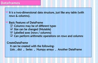
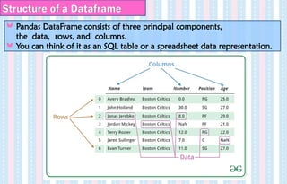
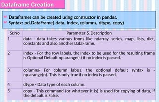
![Creating an empty Dataframe
A basic DataFrame, which can be created is an Empty Dataframe.
>>> import pandas as pd
>>> d=pd.DataFrame()
>>> d
Empty DataFrame
Columns: []
Index: []](https://image.slidesharecdn.com/ln-250918173733-5ea4f2ca/85/Ln-1-Data-Handling-using-Pandas-I-1-pptx-93-320.jpg)

![Creating a Dataframe from lists with values only
The DataFrame can be created using a single list or a list of lists.
CREATING A DATAFRAME FROM SINGLE LIST
Example1:
import pandas as pd
data = [1,2,3,4,5]
df = pd.DataFrame(data)
print (df)](https://image.slidesharecdn.com/ln-250918173733-5ea4f2ca/85/Ln-1-Data-Handling-using-Pandas-I-1-pptx-95-320.jpg)
![Creating a Dataframe from lists of lists (multidimensional list)
CREATE A DATAFRAME FROM A LIST OF LISTS
import pandas as pd
data = [['Alex',10],['Bob',12],['Clarke',13]]
df = pd.DataFrame(data,columns=['Name','Age'])
print (df)
Name Age
0 Alex 10
1 Bob 12
2 Clarke 13](https://image.slidesharecdn.com/ln-250918173733-5ea4f2ca/85/Ln-1-Data-Handling-using-Pandas-I-1-pptx-96-320.jpg)
![Creating a Dataframe from lists of lists (multidimensional list)
import pandas as pd
>>> a=[12,13,14,15]
>>> b=[20,30,40,50]
>>> c=pd.DataFrame(a,index=[b],columns=['Numbers'],dtype='float')
>>> c
Numbers
20 12.0
30 13.0
40 14.0
50 15.0](https://image.slidesharecdn.com/ln-250918173733-5ea4f2ca/85/Ln-1-Data-Handling-using-Pandas-I-1-pptx-97-320.jpg)
![Example
>>> data = [[0, 1, 2],[3, 4, 5]]
>>> df = pd.DataFrame(data)
>>> df
0 1 2
0 0 1 2
1 3 4 5](https://image.slidesharecdn.com/ln-250918173733-5ea4f2ca/85/Ln-1-Data-Handling-using-Pandas-I-1-pptx-98-320.jpg)
![Creating a Dataframe from lists of lists (multidimensional list)
Using multi-dimensional list with column name and dtype
specified.
import pandas as pd
lst = [['tom', 'reacher', 25], ['krish', 'pete', 30],
['nick', 'wilson', 26], ['juli', 'williams', 22]]
df = pd.DataFrame(lst, columns =['FName', 'LName', 'Age'],
dtype = float)
df](https://image.slidesharecdn.com/ln-250918173733-5ea4f2ca/85/Ln-1-Data-Handling-using-Pandas-I-1-pptx-99-320.jpg)
![Program
Display the following details in a dataframe.
Name Marks Index
Vijaya 80 B1
Rahul 92 A2
Meghna 67 C
Radhika 95 A1
Shaurya 97 A1
df = pd.DataFrame(lst, columns =['FName', 'LName', 'Age'], dtype = float)](https://image.slidesharecdn.com/ln-250918173733-5ea4f2ca/85/Ln-1-Data-Handling-using-Pandas-I-1-pptx-100-320.jpg)
![Displaying index and col
>>> df = pd.DataFrame([[0, 1, 2], [3, 4, 5]], index=['row1',
'row2'],columns=['col1', 'col2', 'col3'])
>>> df
col1 col2 col3
row1 0 1 2
row2 3 4 5
>>> print(df.index)
Index(['row1', 'row2'], dtype='object')
>>> print(df.columns)
Index(['col1', 'col2', 'col3'], dtype='object')](https://image.slidesharecdn.com/ln-250918173733-5ea4f2ca/85/Ln-1-Data-Handling-using-Pandas-I-1-pptx-101-320.jpg)
![Creating DataFrames from Series
DataFrames are 2 dimensional representation of Series.
When we represent 2 or more series in the form of rows and columns,
it becomes a dataframe.
Lets create 2 series and pass it into a dataframe.
>>> p={'one':pd.Series([1,2,3], index=['a','b','c']), 'two':pd.Series
([11,22,33,44], index=['a','b','c','d'])}
>>> q=pd.DataFrame(p)
>>> q
one two
a 1.0 11
b 2.0 22
c 3.0 33
d NaN 44](https://image.slidesharecdn.com/ln-250918173733-5ea4f2ca/85/Ln-1-Data-Handling-using-Pandas-I-1-pptx-102-320.jpg)
![>>> p=pd.Series([10,20,30],index=['a','b','c'])
>>> q=pd.Series([40,50,60],index=['a','b','c'])
>>> r=pd.DataFrame({'Set1':p , 'Set2':q})
>>> r
Set1 Set2
a 10 40
b 20 50
c 30 60
Creating DataFrames from Series](https://image.slidesharecdn.com/ln-250918173733-5ea4f2ca/85/Ln-1-Data-Handling-using-Pandas-I-1-pptx-103-320.jpg)
![Creating DataFrames from Series
# To create dataframe from 2 series of student data
import pandas as pd
stud_marks=pd.Series([89,94,93,83,89],index=['Anuj','Deepak','Sohail'
,'Tresa','Hima'])
stud_age=pd.Series([18,17,19,16,18],index=['Anuj','Deepak','Sohail','Tre
sa','Hima'])
>>> stud=pd.DataFrame({'Marks':stud_marks,'Age':stud_age})
>>> stud
Marks Age
Anuj 89 18
Deepak 94 17
Sohail 93 19
Tresa 83 16
Hima 89 18](https://image.slidesharecdn.com/ln-250918173733-5ea4f2ca/85/Ln-1-Data-Handling-using-Pandas-I-1-pptx-104-320.jpg)
![Sorting data in DataFrames
We can sort the data inside a dataframe using sort_values().
Here 2 arguments are passed- sorting field and the order of sorting (asc
or desc).
‘By’ keyword, defines the name of the field or column based on which
it is to be sorted.
>>> stud.sort_values(by=['Marks'])
Marks Age
Tresa 83 16
Anuj 89 18
Hima 89 18
Sohail 93 19
Deepak 94 17
stud.sort_values(by=['Marks'],ascending=False)
Marks Age
Deepak 94 17
Sohail 93 19
Anuj 89 18
Hima 89 18
Tresa 83 16](https://image.slidesharecdn.com/ln-250918173733-5ea4f2ca/85/Ln-1-Data-Handling-using-Pandas-I-1-pptx-105-320.jpg)
![Creating DataFrame from Dictionary (Dictionary of Lists)
• List of dictionaries can be passed as an input data to create a dataframe.
• The dictionary keys are by default, taken as column names.
import pandas as pd
data = {'Name':['Tom', 'Jack', 'Steve', 'Ricky'],'Age':[28,34,29,42]}
df = pd.DataFrame(data)
print (df)
Age Name
0 28 Tom
1 34 Jack
2 29 Steve
3 42 Ricky](https://image.slidesharecdn.com/ln-250918173733-5ea4f2ca/85/Ln-1-Data-Handling-using-Pandas-I-1-pptx-106-320.jpg)
![Program
cars = {'Brand': ['Honda Civic','Toyota Corolla','Ford Focus','Audi A4'],
'Price': [22000,25000,27000,35000] }
df = pd.DataFrame(cars, columns = ['Brand', 'Price'])
print (df)
Brand Price
0 Honda Civic 22000
1 Toyota Corolla 25000
2 Ford Focus 27000
3 Audi A4 35000
Brand Price
car1 Honda Civic 22000
car2 Toyota Corolla 25000
car3 Ford Focus 27000
car4 Audi A4 35000](https://image.slidesharecdn.com/ln-250918173733-5ea4f2ca/85/Ln-1-Data-Handling-using-Pandas-I-1-pptx-107-320.jpg)
![import pandas as pd
data = { ‘Name ‘ : [ ‘Tom’,’Jack’,’Steve’,’Ricky’], ‘Age’ : [28,34,29,42] }
df = pd.DataFrame (data, index = [‘rank 1’, ‘rank 2’, ‘rank 3’, ‘rank 4’ ])
print ( df )
output
AGE NAME
RANK 1 28 tOM
RANK 2 34 jACK
RANK 3 29 Steve
RANK 4 42 Ricky
Program - Create an indexed DataFrame](https://image.slidesharecdn.com/ln-250918173733-5ea4f2ca/85/Ln-1-Data-Handling-using-Pandas-I-1-pptx-108-320.jpg)

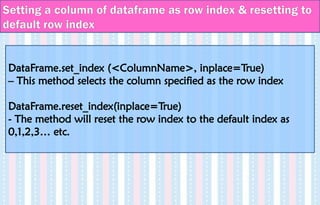
![Suppose we want to make one of the columns as row index:
import pandas as pd
data = {'Name':['Tom', 'Jack', 'Steve', 'Ricky'],'Age':[28,34,29,42]}
df = pd.DataFrame(data)
df.set_index('Name',inplace=True)
print (df)
Age
Name
Tom 28
Jack 34
Steve 29
Ricky 42
Example](https://image.slidesharecdn.com/ln-250918173733-5ea4f2ca/85/Ln-1-Data-Handling-using-Pandas-I-1-pptx-111-320.jpg)
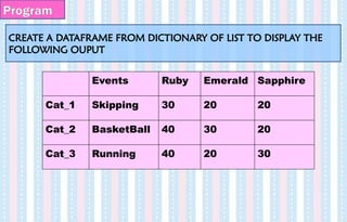
![# Create a DataFrame from List of Dictionaries
import pandas as pd
data1 = [{'x': 1, 'y': 2},{'x': 5, 'y': 4, 'z':5}]
df1 =pd.DataFrame(data1)
x y z
0 1 2 NaN
1 5 4 5.0
Note − Observe, NaN (Not a Number) is appended in missing
areas.
Program](https://image.slidesharecdn.com/ln-250918173733-5ea4f2ca/85/Ln-1-Data-Handling-using-Pandas-I-1-pptx-113-320.jpg)
![Create a DataFrame with a list of dictionaries, row indices, and
column indices.
import pandas as pd
data = [{'a': 1, 'b': 2},{'a': 5, 'b': 10, 'c': 20}]
df1 = pd.DataFrame(data, index=['first', 'second'], columns=['a',
'b‘,’c’])
>>> df1
a b c
first 1 2 NaN
second 5 10 20.0
Program](https://image.slidesharecdn.com/ln-250918173733-5ea4f2ca/85/Ln-1-Data-Handling-using-Pandas-I-1-pptx-114-320.jpg)
![ Create a series from a one list containing authors name and another list
containing number of articles written.
Create a dataframe from the series created using a dictionary containing key as
“Authors” and “Articles”
The following output must be obtained:
Program
import pandas as pd
a=["Jitender","Purnima","Arpit","Jyoti"]
b=[210,211,114,178]
s = pd.Series(a)
s1= pd.Series(b)
df=pd.DataFrame({"Author":s,"Article":s1})
df](https://image.slidesharecdn.com/ln-250918173733-5ea4f2ca/85/Ln-1-Data-Handling-using-Pandas-I-1-pptx-115-320.jpg)
![• To access and retrieve the records from a dataframe, we need to use slice
operation.
• Slicing will display the retrieved records as per the defined range.
import pandas as pd
student={'Name':['Rinku','Ritu','Ajay','Pankaj','Aditya'], 'English':[84,56,89,
78,36], 'Economics':[96,56,89,45,95], 'IP':[83,85,88,92,97], 'Accounts':
[77,75,63,89,85]}
>>> df=pd.DataFrame(student)
>>> df
Name English Economics IP Accounts
0 Rinku 84 96 83 77
1 Ritu 56 56 85 75
2 Ajay 89 89 88 63
3 Pankaj 78 45 92 89
4 Aditya 36 95 97 85
Selecting & Accessing from DataFrame](https://image.slidesharecdn.com/ln-250918173733-5ea4f2ca/85/Ln-1-Data-Handling-using-Pandas-I-1-pptx-116-320.jpg)
![df[1:4] # Records from 1st
to 3rd
row are displayed
Name English Economics IP Accounts
1 Ritu 56 56 85 75
2 Ajay 89 89 88 63
3 Pankaj 78 45 92 89
Note- Single row accessing is not possible.
To display a whole column,
>>> df['Name']
To display more than 1 columns,
>>> df[['Name','IP']]
>>> df['Name'][0:3]
0 Rinku
1 Ritu
2 Ajay
Name: Name, dtype: object
Selecting & Accessing from DataFrame](https://image.slidesharecdn.com/ln-250918173733-5ea4f2ca/85/Ln-1-Data-Handling-using-Pandas-I-1-pptx-117-320.jpg)
![• Pandas provides us the flexibility to even change or rename any column inside a
dataframe.
• To change for a single column-
df.rename(columns={'Name':'Emp_Name'}, inplace=True)
• Consider a list of age of students-
a1=[20,30,25,26,15]
Rename the column ‘a1’ to ‘age’
>>> a1=[20,30,25,26,15]
>>> a1
[20, 30, 25, 26, 15]
Renaming column in DataFrame
>>> df=pd.DataFrame(a1)
>>> df
0
0 20
1 30
2 25
3 26
4 15
>>> df.columns=['Age']
>>> df
Age
0 20
1 30
2 25
3 26
4 15](https://image.slidesharecdn.com/ln-250918173733-5ea4f2ca/85/Ln-1-Data-Handling-using-Pandas-I-1-pptx-118-320.jpg)
![• To add new columns to an already existing dataframe, the syntax is-
dfobject.colname[row_label]=new_value
>>> df['Age1']=45 # the entire column is filled up with 45
>>> df
Age Age1
0 20 45
1 30 45
2 25 45
3 26 45
4 15 45
Adding column to a DataFrame
df['Age3']=pd.Series([42,35,44,50,60])
df
Age Age2 Age3
0 20 45 42
1 30 45 35
2 25 45 44
3 26 45 50
4 15 45 60
df['Total']=df['Age']+df['Age2']+df['Age3']
df
Age Age2 Age3 Total
0 20 45 42 107
1 30 45 35 110
2 25 45 44 114
3 26 45 50 121
4 15 45 60 120](https://image.slidesharecdn.com/ln-250918173733-5ea4f2ca/85/Ln-1-Data-Handling-using-Pandas-I-1-pptx-119-320.jpg)
![• We can update a column values by using arithmetic operators.
• We can also assign or copy the values of a dataframe with the help of assignment
operator.
• To add a new column for updated_age after 10 years for all students,
>>> df['Total']=df['Total']+10
>>> df
Age Age2 Age3 Total
0 20 45 42 117
1 30 45 35 120
2 25 45 44 124
3 26 45 50 131
4 15 45 60 130
>>> df['Updated_Age']=df['Total']
>>> df
Age Age2 Age3 Total Updated_Age
0 20 45 42 117 117
1 30 45 35 120 120
2 25 45 44 124 124
3 26 45 50 131 131
4 15 45 60 130 130
Adding column to a DataFrame](https://image.slidesharecdn.com/ln-250918173733-5ea4f2ca/85/Ln-1-Data-Handling-using-Pandas-I-1-pptx-120-320.jpg)
![1. Create a dataframe from the dictionary of list.
Name Height Qualification
0 Jai 5.1 Msc
1 Princi 6.2 MA
2 Gaurav 5.1 Msc
3 Anuj 5.2 Msc
2. Add a column address to the dataframe with values:
address = ['Delhi', 'Bangalore', 'Chennai', 'Patna']
Sample Question-](https://image.slidesharecdn.com/ln-250918173733-5ea4f2ca/85/Ln-1-Data-Handling-using-Pandas-I-1-pptx-121-320.jpg)
![data = {'Name': ['Jai', 'Princi', 'Gaurav', 'Anuj'],'Height': [5.1, 6.2, 5.1,
5.2],'Qualification': ['Msc', 'MA', 'Msc', 'Msc']}
df = pd.DataFrame(data)
>>> df['address']=['Delhi', 'Bangalore', 'Chennai', 'Patna']
>>> df
Name Height Qualification address
0 Jai 5.1 Msc Delhi
1 Princi 6.2 MA Bangalore
2 Gaurav 5.1 Msc Chennai
3 Anuj 5.2 Msc Patna
Sample Question-](https://image.slidesharecdn.com/ln-250918173733-5ea4f2ca/85/Ln-1-Data-Handling-using-Pandas-I-1-pptx-122-320.jpg)
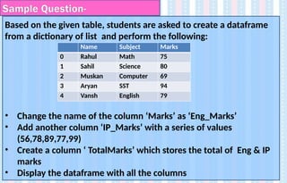
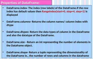

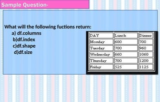
![import pandas as pd
df = pd.DataFrame({'Date':['10/2/2011', '11/2/2011', '12/2/2011',
'13/2/11'], 'Event':['Music', 'Poetry', 'Theatre', 'Comedy'], 'Cost':
[10000, 5000, 15000, 2000]})
print (df)
print(df.index)
print(df.columns)
print(df.dtype)
print(df.size)
print(df.shape)
Sample Question-](https://image.slidesharecdn.com/ln-250918173733-5ea4f2ca/85/Ln-1-Data-Handling-using-Pandas-I-1-pptx-127-320.jpg)
![• The method of selecting / accessing a column of a dataframe is
similar to slicing using series.
• Pandas provides 3 methods to access dataframe column(s)
Using the format of square brackets followed by the name of the
column passed as a string value, like
df_object.[‘column_name’]
Using the dot notation df_object.column_name
Using numeric indexing and the iloc attribute, like
df_object.iloc[:,<column_number>]
• Here , i stands for integer, which signifies that this command shall
return a numeric value denoting the row and column range
SELECTING A COLUMN FROM A DATAFRAME](https://image.slidesharecdn.com/ln-250918173733-5ea4f2ca/85/Ln-1-Data-Handling-using-Pandas-I-1-pptx-128-320.jpg)
![• Example-
df[‘Total’] and df.Total will give the same output.
SELECTING A COLUMN FROM A DATAFRAME](https://image.slidesharecdn.com/ln-250918173733-5ea4f2ca/85/Ln-1-Data-Handling-using-Pandas-I-1-pptx-129-320.jpg)
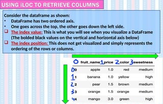
![USING iLOC TO RETRIEVE COLUMNS
Vertical Index Values: [0, 1, 2, 3, 4]
Vertical Index Positions: [0, 1, 2, 3, 4]
Horizontal Index Values: [‘fruit_name’, ‘price, ‘color’, ‘sweetness’]
Horizontal Index Positions: [0, 1, 2, 3]](https://image.slidesharecdn.com/ln-250918173733-5ea4f2ca/85/Ln-1-Data-Handling-using-Pandas-I-1-pptx-131-320.jpg)
![USING iLOC TO RETRIEVE COLUMNS
iloc allows us to index a DataFrame in the same way that we
can index a list; based on index position.
The difference is that a DataFrame has a two-dimensional
index, so we need to pass in slicers for the rows first and
then for the columns.
There are four 4 possible types of slicers we can use on the
table given:
• Scalar positions (eg:- 0,3,4)
• Range of positions (eg:- 0:1, 1:4)
• All positions (:)
• List of positions (eg:- [0,3] , [1,5])](https://image.slidesharecdn.com/ln-250918173733-5ea4f2ca/85/Ln-1-Data-Handling-using-Pandas-I-1-pptx-132-320.jpg)
![If we want to select the data in row 2 and column 0 (i.e., row
index 2 and column index 0) we’ll use the following code:
df.iloc[2,0]
USING iloc- Integer locate](https://image.slidesharecdn.com/ln-250918173733-5ea4f2ca/85/Ln-1-Data-Handling-using-Pandas-I-1-pptx-133-320.jpg)
![Example - USING iloc- Integer locate
>>> df = pd.DataFrame({'Date':['10/2/2011', '11/2/2011', '12/2/2011',
'13/2/11'], 'Event':['Music', 'Poetry', 'Theatre', 'Comedy'], 'Cost':[10000, 5000,
15000, 2000]})
>>> df
Date Event Cost
0 10/2/2011 Music 10000
1 11/2/2011 Poetry 5000
2 12/2/2011 Theatre 15000
3 13/2/11 Comedy 2000
>>> df.iloc[1,1]
'Poetry'
>>> df.iloc[-1,0]
'13/2/11'
>>> df.iloc[2,2]
15000](https://image.slidesharecdn.com/ln-250918173733-5ea4f2ca/85/Ln-1-Data-Handling-using-Pandas-I-1-pptx-134-320.jpg)
![Example - USING iloc- Integer locate
>>> df = pd.DataFrame({'Date':['10/2/2011', '11/2/2011', '12/2/2011', '13/2/11'],
'Event':['Music', 'Poetry', 'Theatre', 'Comedy'], 'Cost':[10000, 5000, 15000, 2000]})
>>> df
Date Event Cost
0 10/2/2011 Music 10000
1 11/2/2011 Poetry 5000
2 12/2/2011 Theatre 15000
3 13/2/11 Comedy 2000
>>> df.iloc[2:4,0:3]
Date Event Cost
2 12/2/2011 Theatre 15000
3 13/2/11 Comedy 2000](https://image.slidesharecdn.com/ln-250918173733-5ea4f2ca/85/Ln-1-Data-Handling-using-Pandas-I-1-pptx-135-320.jpg)
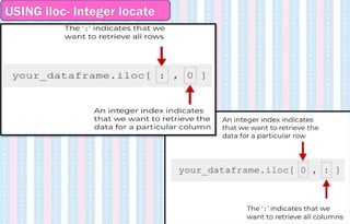
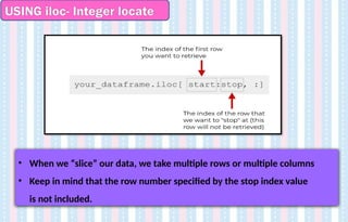
![Example - USING iloc- Integer locate
>>> df
>>> df
Date Event Cost
0 10/2/2011 Music 10000
1 11/2/2011 Poetry 5000
2 12/2/2011 Theatre 15000
3 13/2/11 Comedy 2000
>>> df.iloc[:,:]
Date Event Cost
0 10/2/2011 Music 10000
1 11/2/2011 Poetry 5000
2 12/2/2011 Theatre 15000
3 13/2/11 Comedy 2000
>>> df.iloc[:,0:2]
Date Event
0 10/2/2011 Music
1 11/2/2011 Poetry
2 12/2/2011 Theatre
3 13/2/11 Comedy
>>> df.iloc[0:2,:]
Date Event Cost
0 10/2/2011 Music 10000
1 11/2/2011 Poetry 5000](https://image.slidesharecdn.com/ln-250918173733-5ea4f2ca/85/Ln-1-Data-Handling-using-Pandas-I-1-pptx-138-320.jpg)
![USING iloc- Integer locate
>>> df
Date Event Cost
0 10/2/2011 Music 10000
1 11/2/2011 Poetry 5000
2 12/2/2011 Theatre 15000
3 13/2/11 Comedy 2000
>>> df.iloc[[0,3],[0,1]]
Date Event
0 10/2/2011 Music
4 13/2/11 Comedy
>>> df.iloc[[0,3],[0,2]]
Date Cost
0 10/2/2011 10000
3 13/2/11 2000](https://image.slidesharecdn.com/ln-250918173733-5ea4f2ca/85/Ln-1-Data-Handling-using-Pandas-I-1-pptx-139-320.jpg)
![USING iloc- Integer locate
To display only columns Date and Cost,
>>> df[['Date','Cost']]
Date Cost
0 10/2/2011 10000
1 11/2/2011 5000
2 12/2/2011 15000
3 13/2/11 2000
>>> df.iloc[:,[0,2]]
Date Cost
0 10/2/2011 10000
1 11/2/2011 5000
2 12/2/2011 15000
3 13/2/11 2000](https://image.slidesharecdn.com/ln-250918173733-5ea4f2ca/85/Ln-1-Data-Handling-using-Pandas-I-1-pptx-140-320.jpg)


![DELETING A COLUMN FROM A DATAFRAME
• Using del keyword – [ONLY FOR COLUMN , 1 column at a time]
del df[‘<column name>’]
This will only delete the particular column , after which we have to display the
dataframe to see the changes.
>>> del df['Date']
>>> df
Event Cost
0 Music 10000
1 Poetry 5000
2 Theatre 15000
3 Comedy 2000](https://image.slidesharecdn.com/ln-250918173733-5ea4f2ca/85/Ln-1-Data-Handling-using-Pandas-I-1-pptx-143-320.jpg)
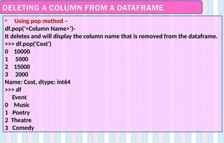
![DELETING A ROW OR COLUMN FROM A DATAFRAME
• Using drop method – drop (labels, axis=1)
It will return a new dataframe with the columns deleted. Axis=1 means column
and axis=0 means row. By default it is 0.
To remove any row,
>>> df.drop([0]) OR >>> df.drop([0],axis=0)
Date Event Cost
1 11/2/2011 Poetry 5000
2 12/2/2011 Theatre 15000
3 13/2/11 Comedy 2000
To remove any column,
>>> df.drop(['Date'],axis=1)
Event Cost
0 Music 10000
1 Poetry 5000
2 Theatre 15000
4 Comedy 2000
To remove a column permanently from your dataframe
you will need to provide one more parameter
inplace=True.](https://image.slidesharecdn.com/ln-250918173733-5ea4f2ca/85/Ln-1-Data-Handling-using-Pandas-I-1-pptx-145-320.jpg)
![DELETING A ROW OR COLUMN FROM A DATAFRAME
• To delete multiple columns :
df.drop([‘Column1’, ‘Column2’], axis=1, inplace = True)
OR
df.drop(columns=[‘Column1’, ‘Column2’], axis=1, inplace = True)
To drop rows :
df.drop([‘row1’,’row2’], axis= 0, inplace = True)
OR
df.drop(index=[‘row1’,’row2’], axis=0, inplace = True)](https://image.slidesharecdn.com/ln-250918173733-5ea4f2ca/85/Ln-1-Data-Handling-using-Pandas-I-1-pptx-146-320.jpg)
![DELETING A COLUMN - Practical Implementation
• Create a simple dataframe with a dictionary of lists, and column
names: name, year, orders, town.
• Remove the column orders from the dataframe using del df[]
• Remove the column ‘name’ using df.pop( )
• Remove the column town using df.drop ()](https://image.slidesharecdn.com/ln-250918173733-5ea4f2ca/85/Ln-1-Data-Handling-using-Pandas-I-1-pptx-147-320.jpg)

![Accessing elements using loc
>>>df = pd.DataFrame({"A":[12, 4, 5, None, 1],"B":[7, 2, 54, 3, None],
"C":[20, 16, 11, 3, 8], "D":[14, 3, None, 2, 6]})
>>> df.iloc[0,2]
20
>>> df.loc[0,'B']
7.0
>>> >>> df.iloc[0:2,0:2]
A B
0 12.0 7.0
1 4.0 2.0
>>> df.loc[0:2,"A":"C"]
A B C
0 12.0 7.0 20
1 4.0 2.0 16
2 5.0 54.0 11](https://image.slidesharecdn.com/ln-250918173733-5ea4f2ca/85/Ln-1-Data-Handling-using-Pandas-I-1-pptx-149-320.jpg)
![Accessing elements using loc
>>> df.iloc[:,0:2]
A B
0 12.0 7.0
1 4.0 2.0
2 5.0 54.0
3 NaN 3.0
4 1.0 NaN
>>> df.loc[:,"A":"C"]
A B C
0 12.0 7.0 20
1 4.0 2.0 16
2 5.0 54.0 11
3 NaN 3.0 3
4 1.0 NaN 8
>>> df.iloc[[1,3],[2,1]]
C B
1 16 2.0
3 3 3.0
>>> df.loc[[1,3],
["A","C"]]
A C
1 4.0 16
3 NaN 3](https://image.slidesharecdn.com/ln-250918173733-5ea4f2ca/85/Ln-1-Data-Handling-using-Pandas-I-1-pptx-150-320.jpg)
![Head and Tail in DataFrame
The method head() gives the first 5
rows and tail gives the last 5.
import pandas as pd
emp={'id':
[100,101,102,103,105,106,107],'na
me':
['Raj','Sini','Flora','Leena','Priya','De
nny','Kevin'],'Sal':
[12000,5000,2200,3200,23000,8700,
15000]}
df=pd.DataFrame(emp)
print(df)
print(df.head())
print(df.tail())
print(df.head(2))
print(df.tail(3))
id name Sal
0 100 Raj 12000
1 101 Sini 5000
2 102 Flora 2200
3 103 Leena 3200
4 105 Priya 23000
5 106 Denny 8700
6 107 Kevin 15000
id name Sal
0 100 Raj 12000
1 101 Sini 5000
2 102 Flora 2200
3 103 Leena 3200
4 105 Priya 23000
id name Sal
2 102 Flora 2200
3 103 Leena 3200
4 105 Priya 23000
5 106 Denny 8700
6 107 Kevin 15000
id name Sal
0 100 Raj 12000
7 101 Sini 5000
id name Sal
4 105 Priya 23000
5 106 Denny 8700
6 107 Kevin 15000](https://image.slidesharecdn.com/ln-250918173733-5ea4f2ca/85/Ln-1-Data-Handling-using-Pandas-I-1-pptx-151-320.jpg)
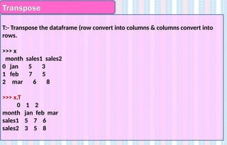
![reindex
Reindex will change the order of index .
>>> x=pd.DataFrame({'month':['jan','feb','mar'], 'sales1':[5,7,6],'sales2':[3,5,8]})
>>> x
month sales1 sales2
0 jan 5 3
1 feb 7 5
2 mar 6 8
>>> y=x.reindex([2,1,0])
>>> y
month sales1 sales2
2 mar 6 8
1 feb 7 5
0 jan 5 3](https://image.slidesharecdn.com/ln-250918173733-5ea4f2ca/85/Ln-1-Data-Handling-using-Pandas-I-1-pptx-153-320.jpg)
![Binary operations
Pandas provides the methods add(), sub(), mul(), div() for carrying out binary
operations on dataframes.
Since all these operations involve 2 dataframes to act upon, they are called
Binary. (‘bi’ means ‘two’ and ‘ary’ means digits)
>>> S1=pd.DataFrame({'UT-1':[23,20,21,19,25],'UT-2':[20,23,12,16,23]})
>>> S2=pd.DataFrame({'UT-1':[13,21,22,10,21],'UT-2':[24,23,11,12,24]})
>>> S1.add(S2)
UT-1 UT-2
0 36 44
1 41 46
2 43 23
3 29 28
4 46 47](https://image.slidesharecdn.com/ln-250918173733-5ea4f2ca/85/Ln-1-Data-Handling-using-Pandas-I-1-pptx-154-320.jpg)
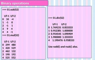
![1.Write the purpose of the following statement:
mtns_df.set_index('name', inplace=True)
2. Write the output of the statement:
a. mtns.loc[:, 'summited’]
b. mtns.loc['K2', :]
c. mtns.loc['K2', 'summited’]
d. mtns.loc[['K2', 'Lhotse'], :]
e. mtns.loc[:, 'height': 'summited’]
f. mtns.loc[mtns.loc[:, 'summited'] > 1954, :]
g. mtns.iloc[0, :]
h. mtns.iloc[:, 2]
i. mtns.iloc[0, 2]
j. mtns.iloc[[1, 3], :]
k. mtns.iloc[:, 0:2]](https://image.slidesharecdn.com/ln-250918173733-5ea4f2ca/85/Ln-1-Data-Handling-using-Pandas-I-1-pptx-156-320.jpg)
![Accessing a DataFrame with a boolean index
• We can create Boolean indexes for dataFrames and searching can be done
based on True or False indexes.
• loc() is used.
• Pandas, DataFrame also support Boolean indexing.
• So we can direct search our data based on True or False indexing.
• We can use loc[ ] for this purpose.
• In order to access a dataframe with a boolean index, we have to create a
dataframe in which index of dataframe contains a boolean value that is
“True” or “False”.
import pandas as pd
dict= {'name':[“Mohak", “Freya", “Roshni"], 'degree': ["MBA", "BCA", "M.Tech"],
'score':[90, 40, 80]}
df= pd.DataFrame(dict, index = [True, False, True])
print(df.loc[True])](https://image.slidesharecdn.com/ln-250918173733-5ea4f2ca/85/Ln-1-Data-Handling-using-Pandas-I-1-pptx-157-320.jpg)
![Accessing a DataFrame with a boolean index
import pandas as pd
data1={ 'rollno' : [101,102,103,104],
'name' : ['ram','mohan','sohan','rohan'] }
student1 = pd.DataFrame(data1,
index = [True, False, True, False],
columns=['rollno' , 'name']
)
print(student1)
Output rollno name
True 101 ram
False 102 mohan
True 103 sohan
False 104 rohan
print(student1.loc[True] )
Output rollno name
True 101 ram
True 103 sohan
-----------------------
print(student1.loc[False] )
Output rollno name
False 102 mohan
False 104 rohan](https://image.slidesharecdn.com/ln-250918173733-5ea4f2ca/85/Ln-1-Data-Handling-using-Pandas-I-1-pptx-158-320.jpg)
![iterrows
• It is used to access the data row wise.
import pandas as pd
ab= [{'Name':'Arya','Age':20},{'Name':'Shane','Age':19}]
df=pd.DataFrame(ab)
for(i,j) in df.iterrows():
print(j)
Name Arya
Age 20
Name: 0, dtype: object
Name Shane
Age 19
Name: 1, dtype: object](https://image.slidesharecdn.com/ln-250918173733-5ea4f2ca/85/Ln-1-Data-Handling-using-Pandas-I-1-pptx-160-320.jpg)
![iteritems
• It is used to access the data column wise.
import pandas as pd
ab= [{'Name':'Arya','Age':20},{'Name':'Shane','Age':19}]
df=pd.DataFrame(ab)
for(i,j) in df.iteritems():
print(j)
0 Arya
1 Shane
Name: Name, dtype: object
0 20
1 19
Name: Age, dtype: int64](https://image.slidesharecdn.com/ln-250918173733-5ea4f2ca/85/Ln-1-Data-Handling-using-Pandas-I-1-pptx-161-320.jpg)
![Basic functions
>>> x=pd.DataFrame({ 'month':
['jan','feb', 'mar'], 'sales1':[5,7,6],
'sales2':[3,5,8]})
>>> x
month sales1 sales2
0 jan 5 3
1 feb 7 5
2 mar 6 8
>>> x.count()
month 3
sales1 3
sales2 3
dtype: int64
>>> x.max()
month mar
sales1 7
sales2 8
dtype: object
>>> x.min()
month feb
sales1 5
sales2 3
dtype: object
>>> x.sum()
month janfebmar
sales1 18
sales2 16
dtype: object](https://image.slidesharecdn.com/ln-250918173733-5ea4f2ca/85/Ln-1-Data-Handling-using-Pandas-I-1-pptx-162-320.jpg)
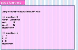
![To fill NaN with desire data in particular column data
import pandas as pd
import numpy as np
data1={'rollno' : [101, 102, 103, 104],
'name' : ['ram','mohan',’sohan’,
np.NaN]}
student1 = pd.DataFrame(data1,
columns=['rollno' , 'name'] )
print(student1)
O/p-
Rollno name
0 101 ram
1 102 mohan
2 103 sohan
3 104 np.NaN
>>> student1 ['name'] . fillna( 'rohit',
inplace = True)
>>> student1
rollno name
0 101 ram
1 102 mohan
2 103 sohan
3 104 rohit
student1. fillna( 999, inplace = True)
print(df)
rollno name
0 101 ram
1 102 mohan
2 103 sohan
3 104 999](https://image.slidesharecdn.com/ln-250918173733-5ea4f2ca/85/Ln-1-Data-Handling-using-Pandas-I-1-pptx-164-320.jpg)
![Adding a new row using - append() method
import pandas as pd
data1={'rollno' : [101,102],
'name' : ['ram','mohan']}
student1 = pd.DataFrame(data1,
columns=['rollno' , 'name'] )
print(student1)
rollno name
0 101 ram
1 102 mohan
#to add a new row in existing a
DataFrame
Student1= student1.append({ 'rollno' :
103, 'name': 'sohan' } ,ignore_index
=True)
print(student1)
rollno name
0 101 ram
1 102 mohan
2 103 sohan](https://image.slidesharecdn.com/ln-250918173733-5ea4f2ca/85/Ln-1-Data-Handling-using-Pandas-I-1-pptx-165-320.jpg)
![Handling missing values (NaN) – dropping Using dropna() method
>>> import pandas as pd
>>>import numpy as np;
>>>data1={'rollno' : [101, 102,
103, 104],'name' :
['ram','mohan','sohan', np.NaN]}
student1 = pd.DataFrame(data1,
columns=['rollno' , 'name'] )
print(student1)
rollno name
0 101 ram
1 102 mohan
2 103 sohan
3 104 NaN
#to drop, all rows of NaN by default
student1 . dropna( inplace = True)
student1
rollno name
0 101 ram
1 102 mohan
2 103 sohan
#to drop, NaN of all column using axis =1
student1 . dropna(axis=1, inplace =
True)
print(student1)](https://image.slidesharecdn.com/ln-250918173733-5ea4f2ca/85/Ln-1-Data-Handling-using-Pandas-I-1-pptx-166-320.jpg)
![To check if zero exists
data1 = {'rollno' : [101, 102, 103, 104],'name' :
['ram', 'mohan', 'sohan', 'rohan']}
student = pd.DataFrame(data1,
columns=['rollno','name'])
print(student)
rollno name
0 101 ram
1 102 mohan
2 103 sohan
3 104 rohan
>>> student.all()
rollno True
name True
dtype: bool
>>> student.all(axis=1)
0 True
1 True
2 True
3 True
dtype: bool
>>> data1 = {'rollno' : [0, 102, 103, 104],'name' :
['ram', 0, 'sohan', 'rohan']}
student = pd.DataFrame(data1,
columns=['rollno','name'])
print(student)
rollno name
0 0 ram
1 102 0
2 103 sohan
3 104 rohan
>>> student.all()
rollno False
name False
dtype: bool
>>> student.all(axis=1)
0 False
1 False
2 True
3 True
dtype: bool
all() returns whether all
elements are True over
the requested axis.](https://image.slidesharecdn.com/ln-250918173733-5ea4f2ca/85/Ln-1-Data-Handling-using-Pandas-I-1-pptx-167-320.jpg)
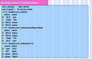
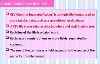

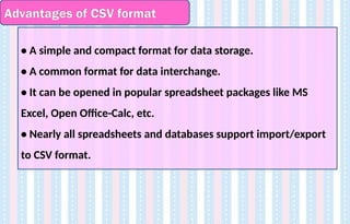


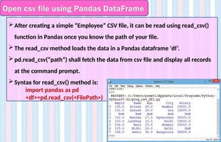
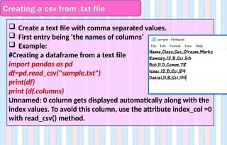
![More commands
• To display the shape (number of rows and columns) of the CSV file
df.shape
>>> df.shape
(7, 5)
Reading CSV file with specific/selected columns-
• This can be done by using “usecols” attribute along with read_csv().
>>> df=pd.read_csv("Employee.csv",usecols=['Name','Age'])
Reading CSV file with specific/selected rows-
• Use “nrows” attribute used with read_csv(). nrows means number of
rows.
>>> df=pd.read_csv("Employee.csv",nrows=5)
• Here 5 rows are displayed. It will display NaN values also, if present.](https://image.slidesharecdn.com/ln-250918173733-5ea4f2ca/85/Ln-1-Data-Handling-using-Pandas-I-1-pptx-179-320.jpg)

![UPDATING/MODIFYING CONTENTS IN A CSV FILE
Reading CSV file with new column names
• Use skiprow option to skip the header if it exists. Specify the new
names with names option.
df=pd.read_csv("Employee.csv",skiprows=1,names=['a','b','c','d','e'])
Replace any contents of the dataframe with NaN values-
• Done by using na_values option along with read_csv method
>>> df=pd.read_csv("Employee.csv",na_values=[26])
Here wherever the value 26 is seen, it gets updated to NaN.](https://image.slidesharecdn.com/ln-250918173733-5ea4f2ca/85/Ln-1-Data-Handling-using-Pandas-I-1-pptx-181-320.jpg)
![Example
import pandas as pd
cars = {'Brand': ['Honda Civic','ToyotaCorolla',
'FordFocus','AudiA4'],'Price': [22000,25000,27000,35000]}
df= pd.DataFrame(cars, columns= ['Brand', 'Price'])
df.to_csv('export_dataframe.csv', index = False, header=True)
#Open the notepad with export_dataframe file.
pd.read_csv('export_dataframe.csv')](https://image.slidesharecdn.com/ln-250918173733-5ea4f2ca/85/Ln-1-Data-Handling-using-Pandas-I-1-pptx-183-320.jpg)


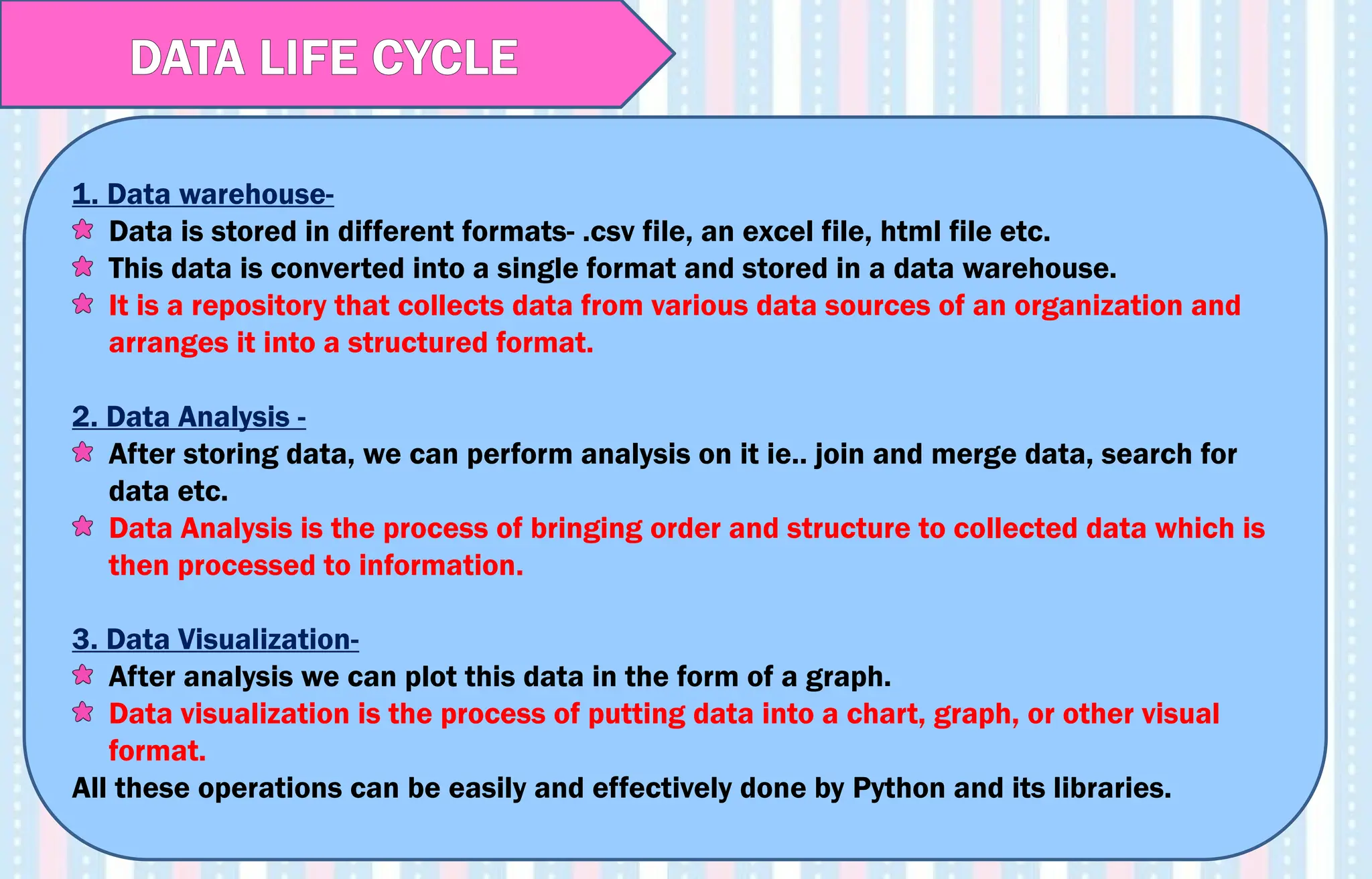
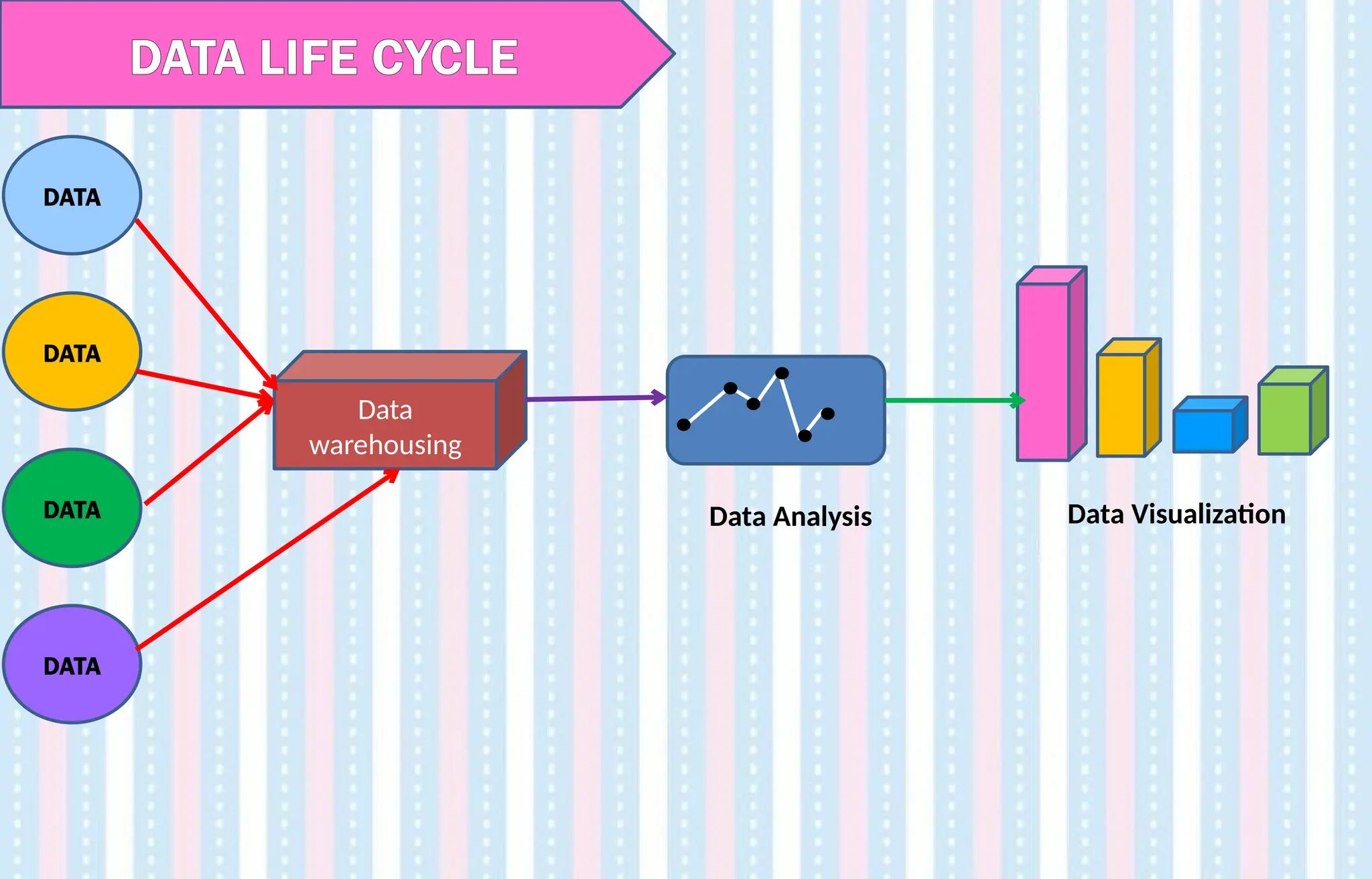
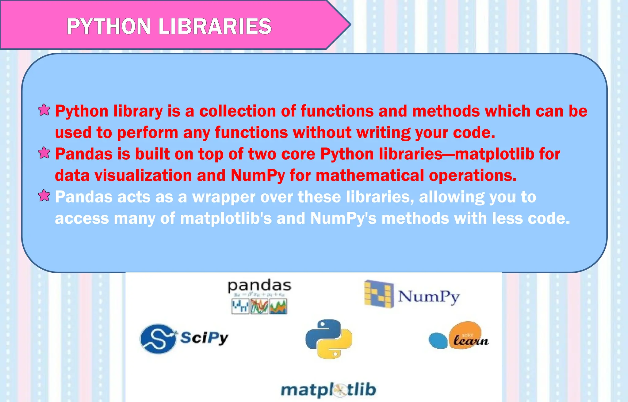
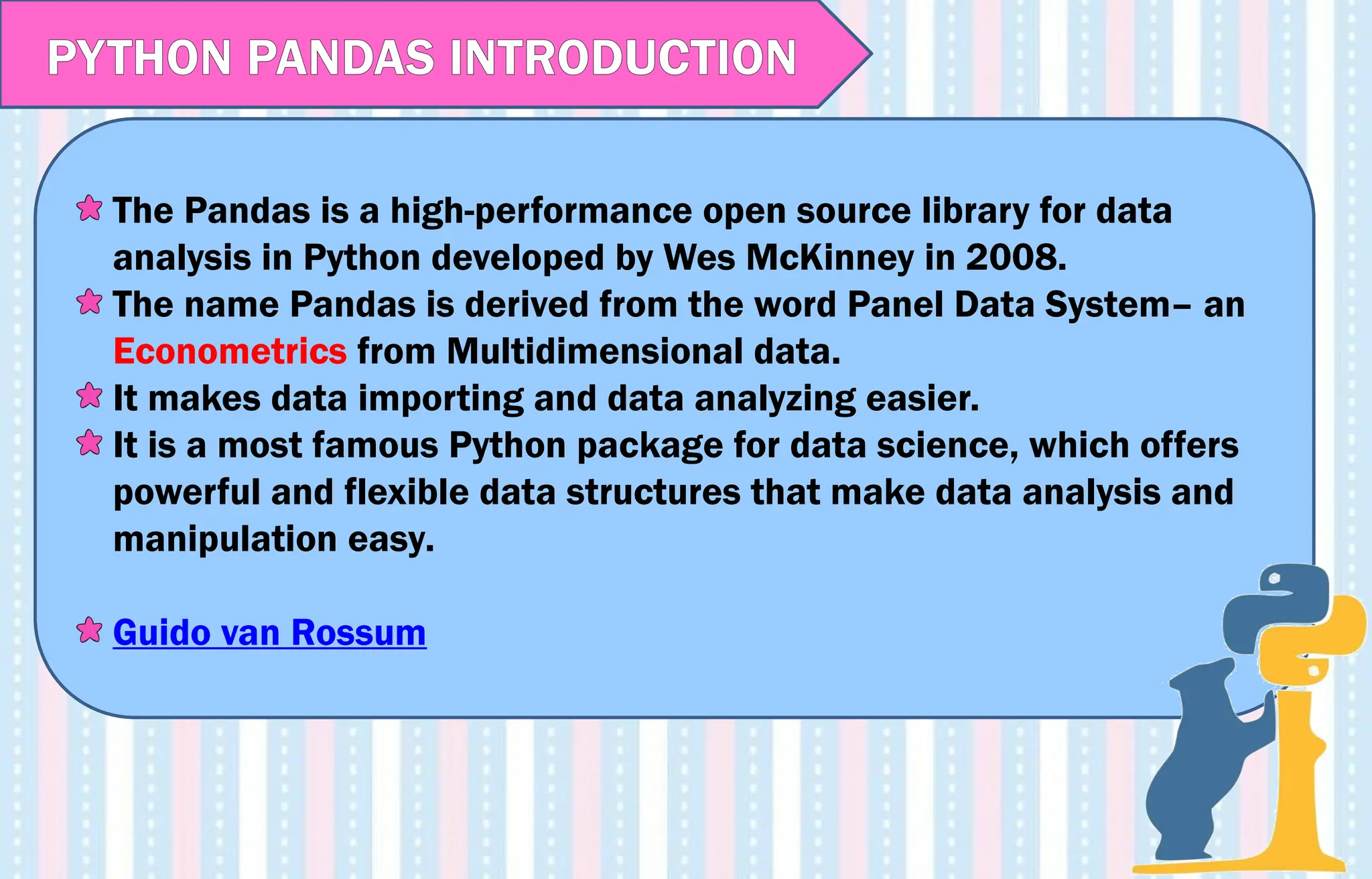

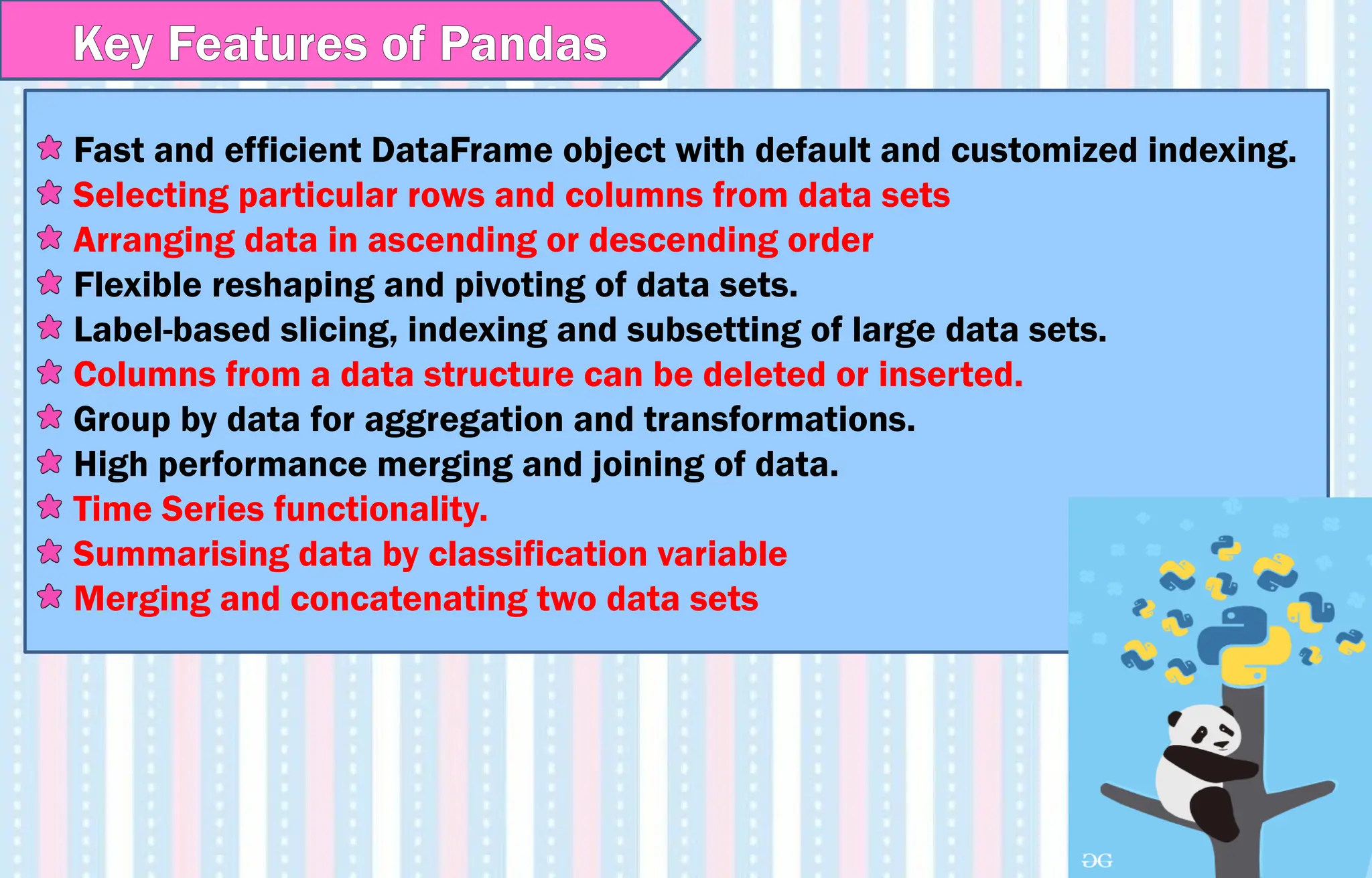

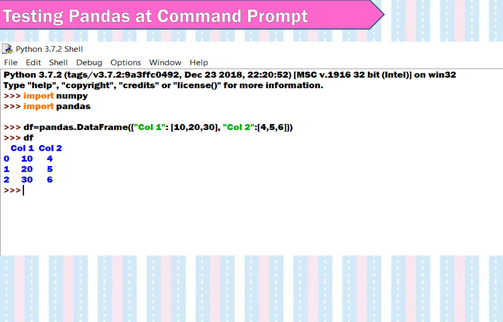
![Pandas Datatypes :
Pandas dtype Python Type NumPy type Usage
object Str String_, unicode_ Text
int64 Int int, int8, int16, int32,
int64, uint8, uint16,
uint32, uint64
Integer
numbers
float64 Float float, float16, float32,
float64
Floating point
numbers
bool bool bool True / False
datetime64 NA datetime64[ns] Date & Time
values](https://image.slidesharecdn.com/ln-250918173733-5ea4f2ca/75/Ln-1-Data-Handling-using-Pandas-I-1-pptx-14-2048.jpg)


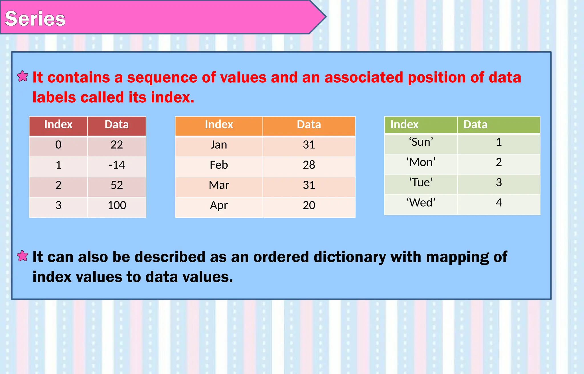
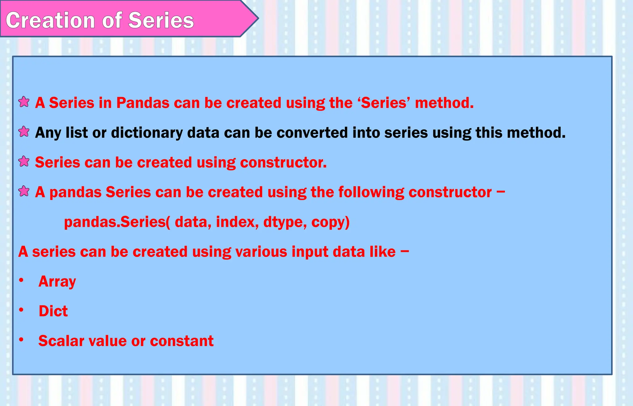
![A basic series, which can be created is an Empty Series.
Example - [Here ‘s’ is the Series Object]
import pandas as pd
s = pd.Series()
print s
Its output is as follows −
Series([], dtype: float64)
Note –
• Series () displays an empty list along with its default data type.
• Pd is an alternate name given to the Pandas module. Its significance is that we
can use ‘pd’ instead of typing Pandas every time we need to use it.
• Import statement is used for loading Pandas module into the memory and can
be used to work with.
Creation of Empty Series](https://image.slidesharecdn.com/ln-250918173733-5ea4f2ca/75/Ln-1-Data-Handling-using-Pandas-I-1-pptx-19-2048.jpg)
![Creating DataSeries with a list
Syntax:
<Series Object>=pandas.Series([data],index=[index])
Eg:-
import pandas as pd
s=pd.Series( [ 2,4,6,8,10])
print(s)
S- is a series variable
Series() – method displays a list along with
default data type
pd is the alternative name given to panda
module
Import statement is used to load pandas
module into the memory and can be used](https://image.slidesharecdn.com/ln-250918173733-5ea4f2ca/75/Ln-1-Data-Handling-using-Pandas-I-1-pptx-20-2048.jpg)
![Program- DataSeries
>>> s= pandas.Series ( [3,-5,7,4] , index=['a','b','c','d‘] )
>>> s
Output:
a 3
b -5
c 7
d 4
dtype: int64](https://image.slidesharecdn.com/ln-250918173733-5ea4f2ca/75/Ln-1-Data-Handling-using-Pandas-I-1-pptx-21-2048.jpg)
![>>> st = pd.Series([20, 70, 10], index=['frog', 'fish', 'hawk'])
>>> st
frog 20
fish 70
hawk 10
dtype: int64
>>> st.index.name = 'Animals'
>>> st
Animals
frog 20
fish 70
hawk 10
dtype: int64
Program](https://image.slidesharecdn.com/ln-250918173733-5ea4f2ca/75/Ln-1-Data-Handling-using-Pandas-I-1-pptx-22-2048.jpg)


![Program
Months=[‘Jan’,’Feb’,’Mar’,’Apr’,’June’, ‘July’]
import pandas as pd
S=pd.Series(Months)
>>> S
0 Jan
1 Feb
2 Mar
3 Apr
4 June
5 July
dtype: object](https://image.slidesharecdn.com/ln-250918173733-5ea4f2ca/75/Ln-1-Data-Handling-using-Pandas-I-1-pptx-25-2048.jpg)
![Accessing Series index and values
#Index and values are attributes of Series.
>>> Months=['Jan','Feb','Mar','Apr','June', 'July']
>>> Months
['Jan', 'Feb', 'Mar', 'Apr', 'June', 'July']
>>> a=pd.Series(Months)
>>> a.index
RangeIndex(start=0, stop=6, step=1)
>>> a.values
array(['Jan', 'Feb', 'Mar', 'Apr', 'June', 'July'], dtype=object)
>>> a.values.tolist()
['Jan', 'Feb', 'Mar', 'Apr', 'June', 'July']](https://image.slidesharecdn.com/ln-250918173733-5ea4f2ca/75/Ln-1-Data-Handling-using-Pandas-I-1-pptx-26-2048.jpg)
![Program
import pandas as ps
games_list = ['Cricket', 'Volleyball', 'Judo', 'Hockey']
abc= ps.Series(games_list)
print(abc)
OUTPUT
0 Cricket
1 Volleyball
2 Judo
3 Hockey
dtype: object](https://image.slidesharecdn.com/ln-250918173733-5ea4f2ca/75/Ln-1-Data-Handling-using-Pandas-I-1-pptx-27-2048.jpg)


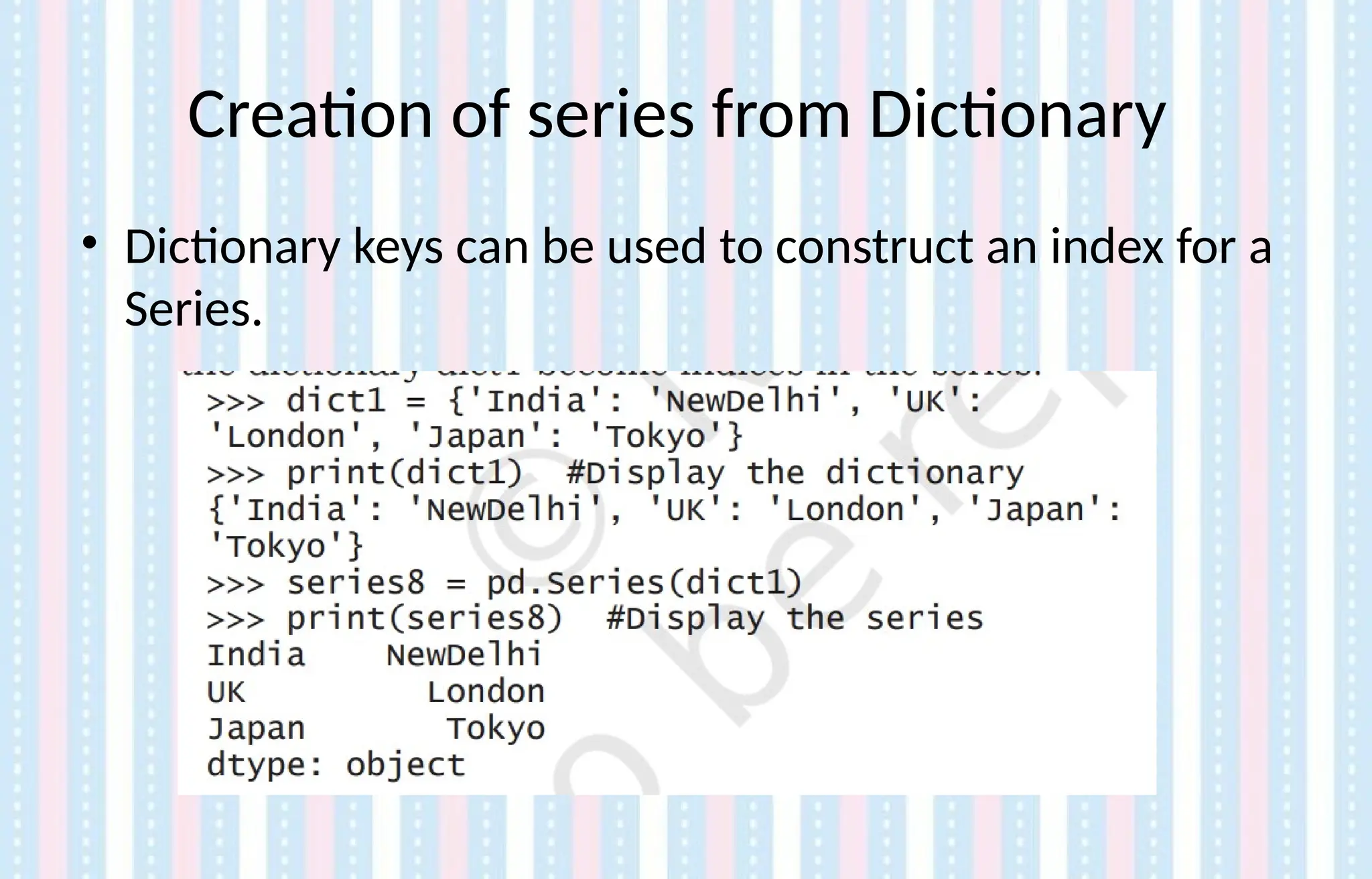
![Attribute of Series
• Series support vector operations.
• Any operation gets performed on every single element.
Eg:-
import pandas as pd
List = [5, 2, 3,7]
s1= pd.Series (List)
Guess the output of these statements:
print (list *2)
print (s1*2)](https://image.slidesharecdn.com/ln-250918173733-5ea4f2ca/75/Ln-1-Data-Handling-using-Pandas-I-1-pptx-31-2048.jpg)

![In Python, one-dimensional structures are displayed as a row of
values. On the contrary, here we see that Series is displayed as a
column of values.
Each cell in Series is accessible via index value along the “axis 0”. For
our Series object indexes are: 0, 1, 2, 3, 4. Here is an example of
accessing different values:
import pandas as pd
N=pd.Series([‘Red’, ‘Green’,’Yellow’,’Orange’, Blue’])
print(N[0])
print (N.axes)
Red
[RangeIndex(start=0, stop=5, step=1)]
Axis in Series](https://image.slidesharecdn.com/ln-250918173733-5ea4f2ca/75/Ln-1-Data-Handling-using-Pandas-I-1-pptx-33-2048.jpg)
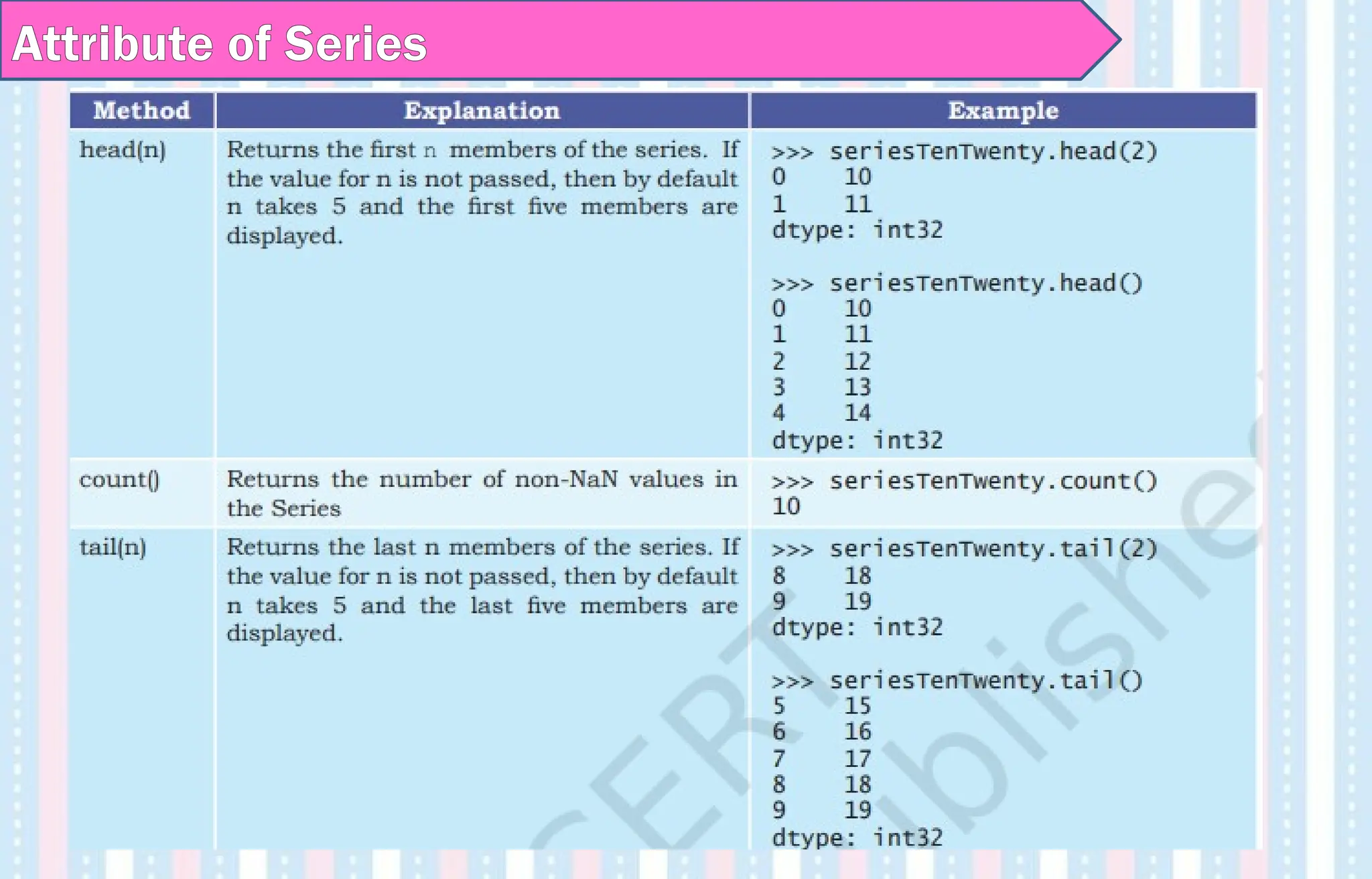
![ACCESSING ROWS USING HEAD () AND TAIL() FUNCTION
Series.head() function will display the top 5 rows in the series.
Series.tail() function will display the last 5 rows in the series
In both the functions, if a number is passed as parameter Pandas will
print the specified number of rows.
Eg:-
>>> a=pd.Series([2,4,6,8,10,12,14,16])
>>> a.head()
0 2
1 4
2 6
3 8
4 10
dtype: int64](https://image.slidesharecdn.com/ln-250918173733-5ea4f2ca/75/Ln-1-Data-Handling-using-Pandas-I-1-pptx-35-2048.jpg)
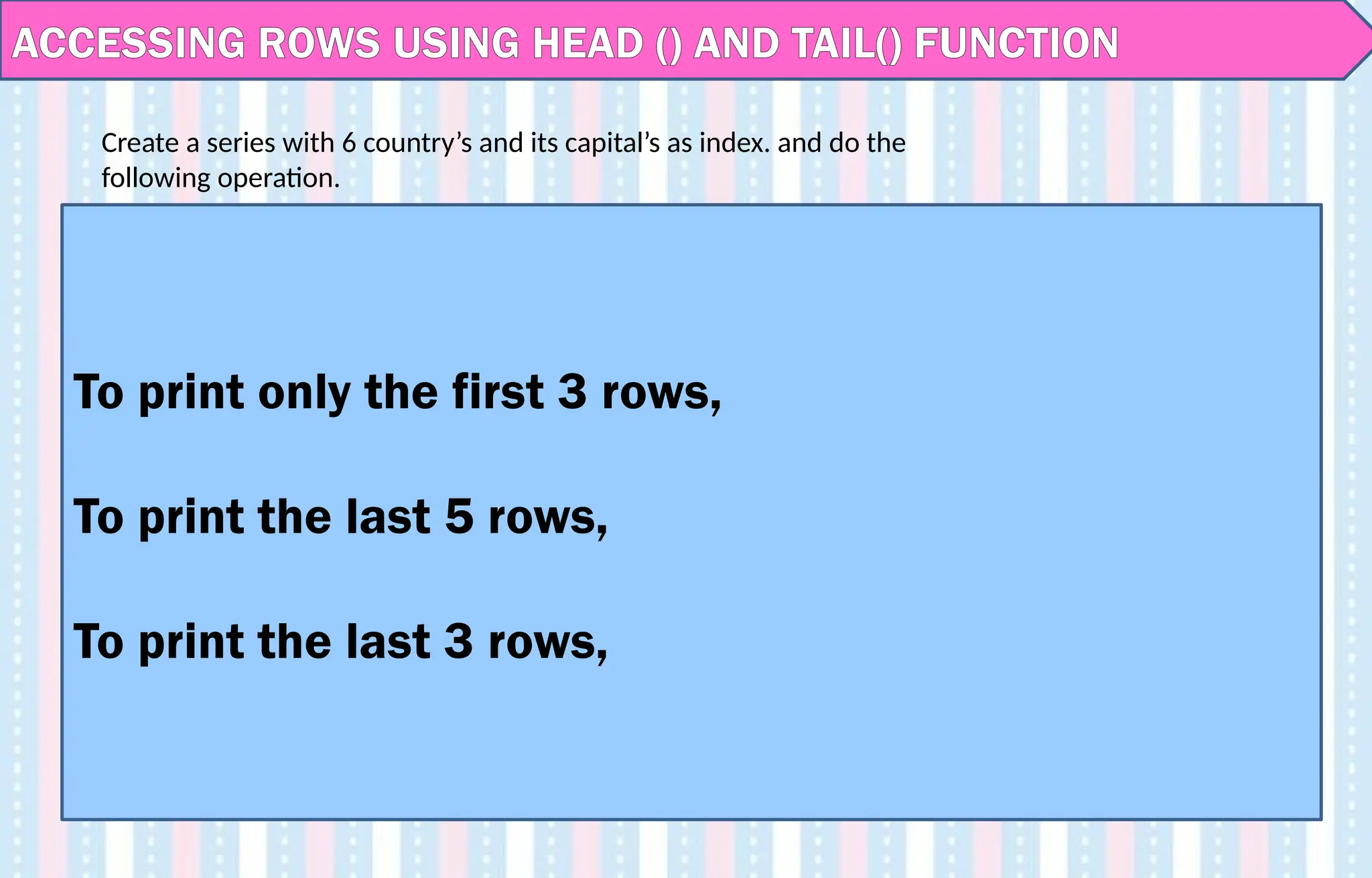
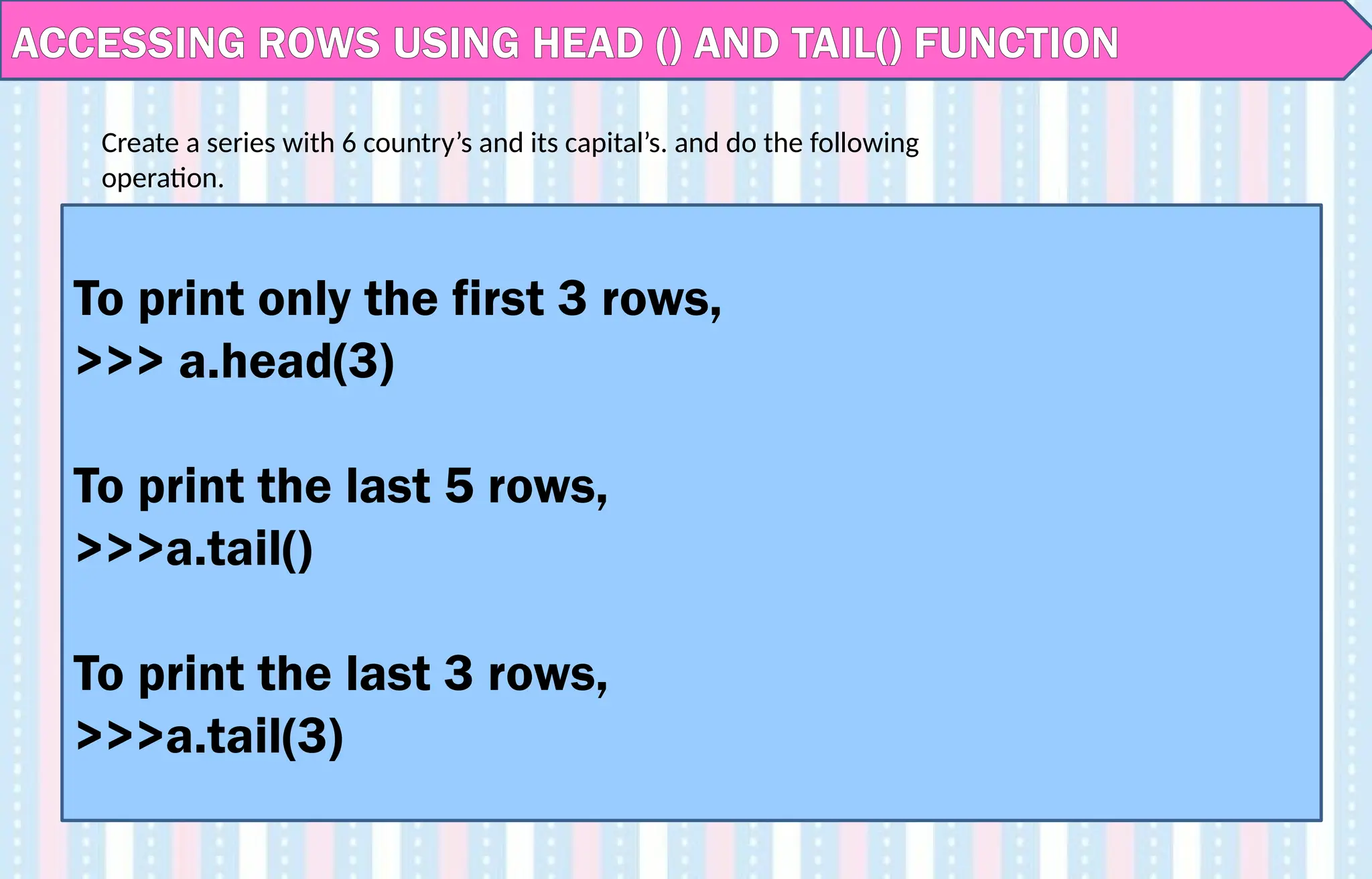
![Vector operations in Series
• Series support vector operations.
• Any operation gets performed on every single element.
Eg:-
import pandas as pd
List = [5, 2, 3,7]
s1= pd.Series (List)
Guess the output of these statements:
print (list *2)
print (s1*2)](https://image.slidesharecdn.com/ln-250918173733-5ea4f2ca/75/Ln-1-Data-Handling-using-Pandas-I-1-pptx-38-2048.jpg)
![Binary operations in Series
>>> import numpy as np
>>> s = pd.Series([1,2,3,4,np.NaN,5,np.NaN])
>>> s
0 1.0
1 2.0
2 3.0
3 4.0
4 NaN
5 5.0
6 NaN
dtype: float64](https://image.slidesharecdn.com/ln-250918173733-5ea4f2ca/75/Ln-1-Data-Handling-using-Pandas-I-1-pptx-40-2048.jpg)
![Write a Pandas program to add, subtract, multiply and divide
two Pandas Series.
Program
import pandas as pd
ds1 = pd.Series([2, 4, 6, 8, 10])
ds2 = pd.Series([1, 3, 5, 7, 9])
ds = ds1 + ds2
print(“Sum of Series: n “ , ds)
ds = ds1 - ds2
print(“Subtraction of Series: n “ , ds)
ds = ds1 * ds2
print(“Product of two Series: n “, ds)
ds = ds1 / ds2
print(“Quotient of the Series: n “ , ds)](https://image.slidesharecdn.com/ln-250918173733-5ea4f2ca/75/Ln-1-Data-Handling-using-Pandas-I-1-pptx-41-2048.jpg)
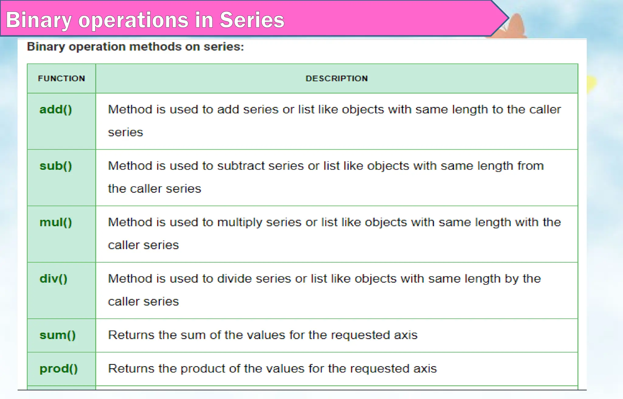
![# importing pandas module
import pandas as pd
# creating a series
data = pd.Series([5, 2, 3,7], index=['a', 'b', 'c', 'd'])
# creating a series
data1 = pd.Series([1, 6, 4, 9], index=['a', 'b', 'd', 'e’])
# add two series using .add() function.
data.add(data1)
Program](https://image.slidesharecdn.com/ln-250918173733-5ea4f2ca/75/Ln-1-Data-Handling-using-Pandas-I-1-pptx-43-2048.jpg)
![Write a Pandas program to compare the elements of the two
Pandas Series.
Program
import pandas as pd
ds1 = pd.Series([2, 4, 6, 8, 10])
ds2 = pd.Series([1, 3, 5, 7, 10])
print("Compare the elements of the said Series:")
print("Equals:")
print(ds1 == ds2)
print("Greater than:")
print(ds1 > ds2)
print("Less than:")
print(ds1 < ds2)](https://image.slidesharecdn.com/ln-250918173733-5ea4f2ca/75/Ln-1-Data-Handling-using-Pandas-I-1-pptx-44-2048.jpg)
![Program – To sort values
abc=pd.Series(['M','A','N','G','O','E','S'],index=[10,20,30,
40,50,60,70])
abc.sort_values()
abc.sort_index()
>>> abc
20 A
60 E
40 G
10 M
30 N
50 O
70 S
dtype: object](https://image.slidesharecdn.com/ln-250918173733-5ea4f2ca/75/Ln-1-Data-Handling-using-Pandas-I-1-pptx-45-2048.jpg)
![Create series from ndarray
An array of values can be passed to a Series.
If data is an ndarray, index must be the same
length as data.
If no index is passed, one will be created having
values [0, ..., len(data) - 1].](https://image.slidesharecdn.com/ln-250918173733-5ea4f2ca/75/Ln-1-Data-Handling-using-Pandas-I-1-pptx-46-2048.jpg)
![Create series from ndarray
import pandas as pd
import numpy as np
data = np.array(['a','b','c','d'])
s = pd.Series(data)
print (s)
Its output is as follows −
0 a
1 b
2 c
3 d
dtype: object
Note- We did not pass any index, so by default, it assigned the indexes ranging
from 0 to len(data)-1, i.e., 0 to 3.](https://image.slidesharecdn.com/ln-250918173733-5ea4f2ca/75/Ln-1-Data-Handling-using-Pandas-I-1-pptx-47-2048.jpg)
![Create series from ndarray
import pandas as pd
import numpy as np
abc = np.array(['a','b','c','d'])
s = pd.Series(abc , index=[100,101,102,103])
print (s)
Its output is as follows −
100 a
101 b
102 c
103 d
dtype: object
We passed the index values here. Now we can see the customized indexed
values in the output.](https://image.slidesharecdn.com/ln-250918173733-5ea4f2ca/75/Ln-1-Data-Handling-using-Pandas-I-1-pptx-48-2048.jpg)
![# To add 5 marks to each student in the series
#creating a series from array and specified index
import pandas as pd
import numpy as np
Marks=np.array([455,478,477,405])
M1=pd.Series(Marks, index=[“Annie", “Resmi", "Sana", “Haya"])
print(M1)
for i, j in M1.items( ): # i – index , j - values
M1.at[i] = j+5 #increase each values
print (M1)
#at - Access a single value for a row/column label pair.
Program – Mathematical operations](https://image.slidesharecdn.com/ln-250918173733-5ea4f2ca/75/Ln-1-Data-Handling-using-Pandas-I-1-pptx-49-2048.jpg)
![import pandas as pd
import numpy as np
a=np.random.randn(5)
>>> a
array([-0.63206378, -0.19692941, 0.3883878 , 0.35998536, 0.1873882 ])
>>> b=pandas.Series(a)
>>> b
0 -0.632064
1 -0.196929
2 0.388388
3 0.359985
4 0.187388
dtype: float64
numpy.random.randn()
Returns an array of defined shape, filled with random floating-point
samples.
Program – random.randn](https://image.slidesharecdn.com/ln-250918173733-5ea4f2ca/75/Ln-1-Data-Handling-using-Pandas-I-1-pptx-50-2048.jpg)
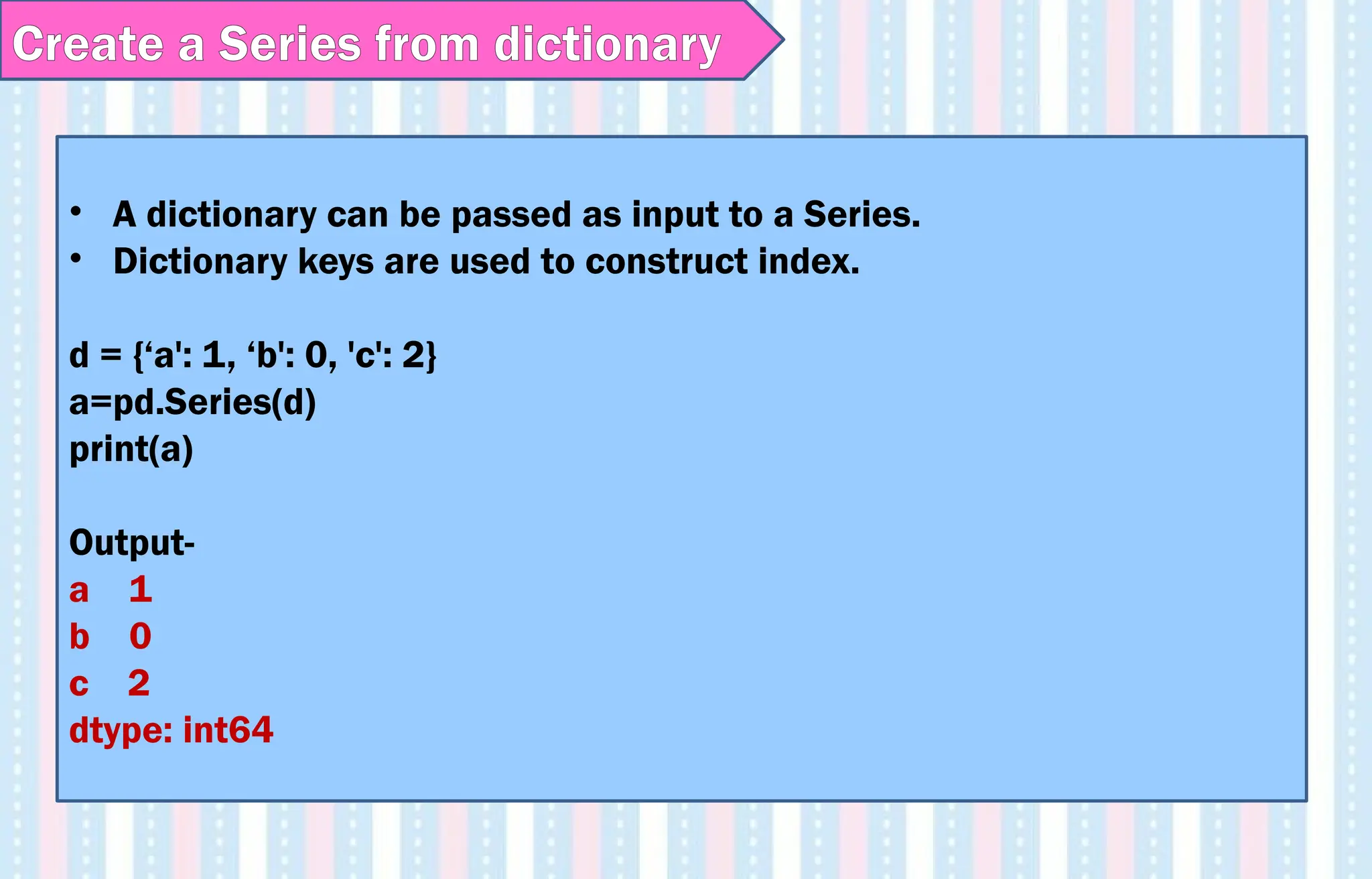

![>>> d3=pd.Series(d1,index=[20,30,40,50,60])
>>> d3
20 NaN
30 NaN
40 NaN
50 NaN
60 NaN
dtype: float64
>>> d4=pd.Series(d1,index=['b','a','c','e','d'])
>>> d4
b 200
a 100
c 300
e 800
d 400
dtype: int64
Create a Series from dictionary](https://image.slidesharecdn.com/ln-250918173733-5ea4f2ca/75/Ln-1-Data-Handling-using-Pandas-I-1-pptx-53-2048.jpg)

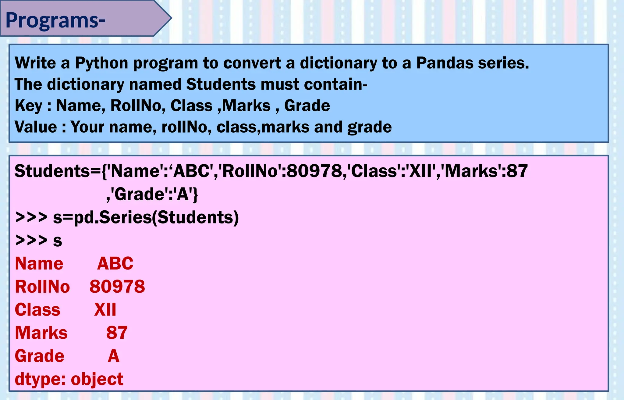
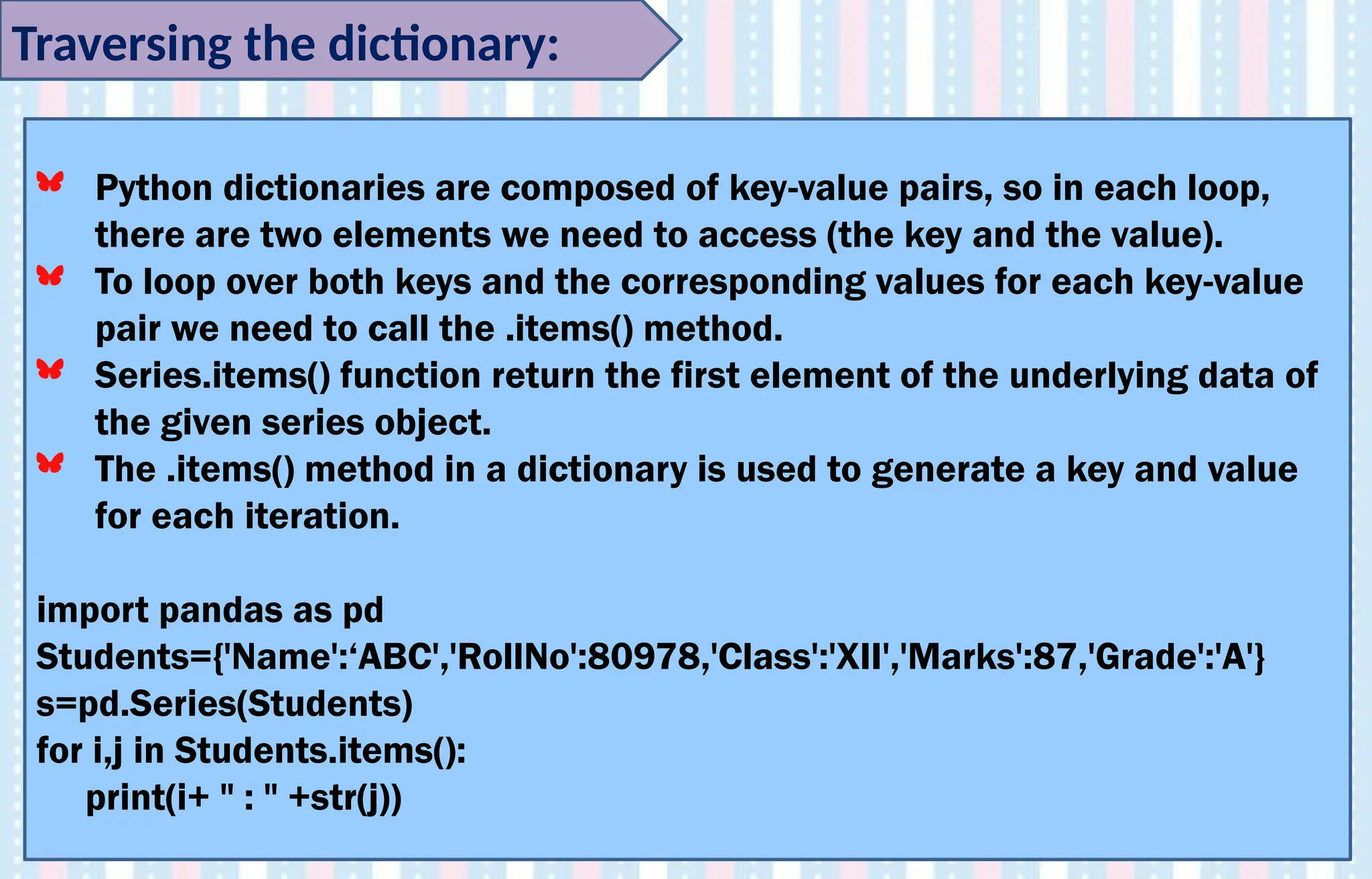
![>>> pers = {'color': 'blue', 'fruit': 'apple', 'pet': 'dog'}
>>> p = pers.items()
>>> p # Here d_items is a view of items
dict_items([('color', 'blue'), ('fruit', 'apple'), ('pet', 'dog')])
>>> for item in pers.items():
print(item)
('color', 'blue')
('fruit', 'apple')
('pet', 'dog')
Traversing a dictionary](https://image.slidesharecdn.com/ln-250918173733-5ea4f2ca/75/Ln-1-Data-Handling-using-Pandas-I-1-pptx-57-2048.jpg)

![Eg. Consider the series created with names of students as index
and Marks as data using dictionary
import pandas as pd
d1={"Raj":234,"Gilbert":345}
m1=pd.Series(d1)
print(m1)
for i,j in m1.items():
m1.at[ i ]=j+5
print(m1)
Mathematical operations on Series](https://image.slidesharecdn.com/ln-250918173733-5ea4f2ca/75/Ln-1-Data-Handling-using-Pandas-I-1-pptx-59-2048.jpg)
![When a scalar is passed, all the elements of the series is
initialized to the same value.
The value will be repeated to match the length of index.
import pandas as pd
s = pd.Series(5, index=[0, 1, 2, 3])
s
Its output is as follows −
0 5
1 5
2 5
3 5
dtype: int64
Create a Series from Scalar](https://image.slidesharecdn.com/ln-250918173733-5ea4f2ca/75/Ln-1-Data-Handling-using-Pandas-I-1-pptx-60-2048.jpg)
![Create a series with scalar value 7 and index as ‘A’,’B’,’C’,’D’
s = pd.Series(7, index=['A','B','C','D'])
>>> s
A 7
B 7
C 7
D 7
dtype: int64
Create a Series from Scalar](https://image.slidesharecdn.com/ln-250918173733-5ea4f2ca/75/Ln-1-Data-Handling-using-Pandas-I-1-pptx-61-2048.jpg)
![Create a Series using string as index
ab = pd.Series(‘Welcome to India’, index=['A','B','C','D'])
>>> s
A Welcome to India
B Welcome to India
C Welcome to India
D Welcome to India
dtype: object](https://image.slidesharecdn.com/ln-250918173733-5ea4f2ca/75/Ln-1-Data-Handling-using-Pandas-I-1-pptx-62-2048.jpg)
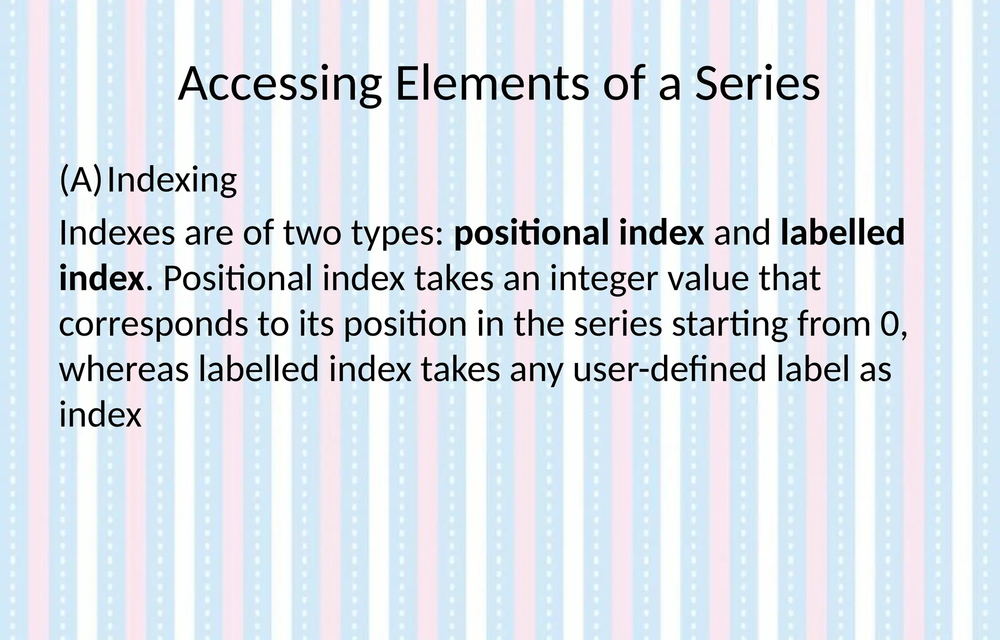
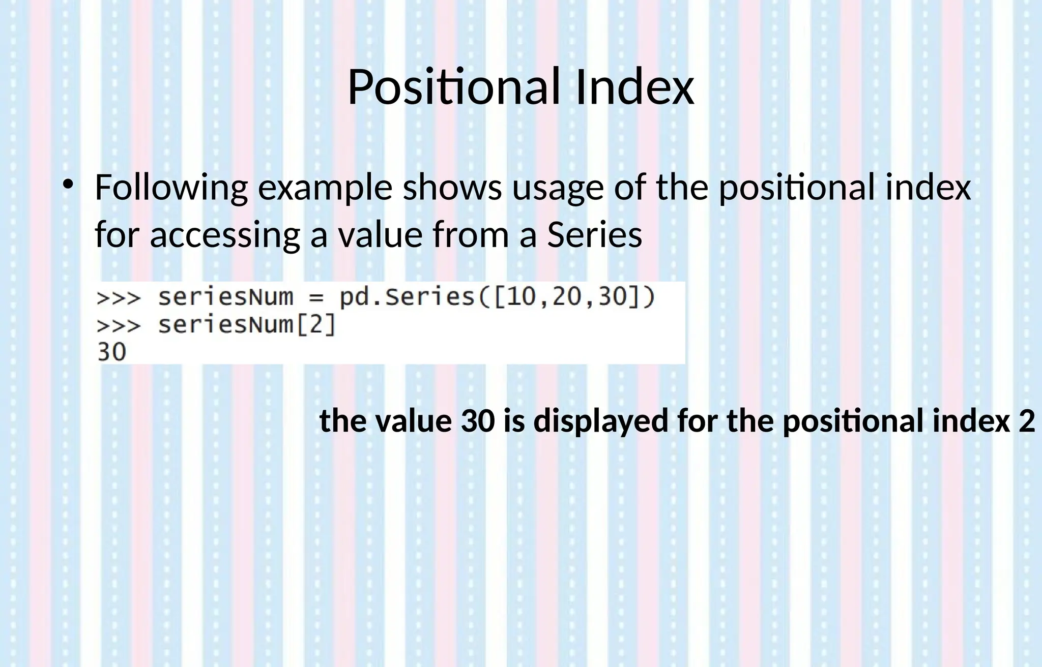
![• More than one element of a series can be accessed using a
list of positional integers or a list of index labels as shown in
the following examples:
>>> seriesCapCntry = pd.Series(['NewDelhi', 'WashingtonDC',
'London', 'Paris'], index=['India', 'USA', 'UK', 'France'])
>>> seriesCapCntry[[3,2]]
France Paris
UK London
dtype: object](https://image.slidesharecdn.com/ln-250918173733-5ea4f2ca/75/Ln-1-Data-Handling-using-Pandas-I-1-pptx-65-2048.jpg)
![>>> seriesCapCntry[['UK','USA']]
UK London
USA WashingtonDC
dtype: object](https://image.slidesharecdn.com/ln-250918173733-5ea4f2ca/75/Ln-1-Data-Handling-using-Pandas-I-1-pptx-66-2048.jpg)
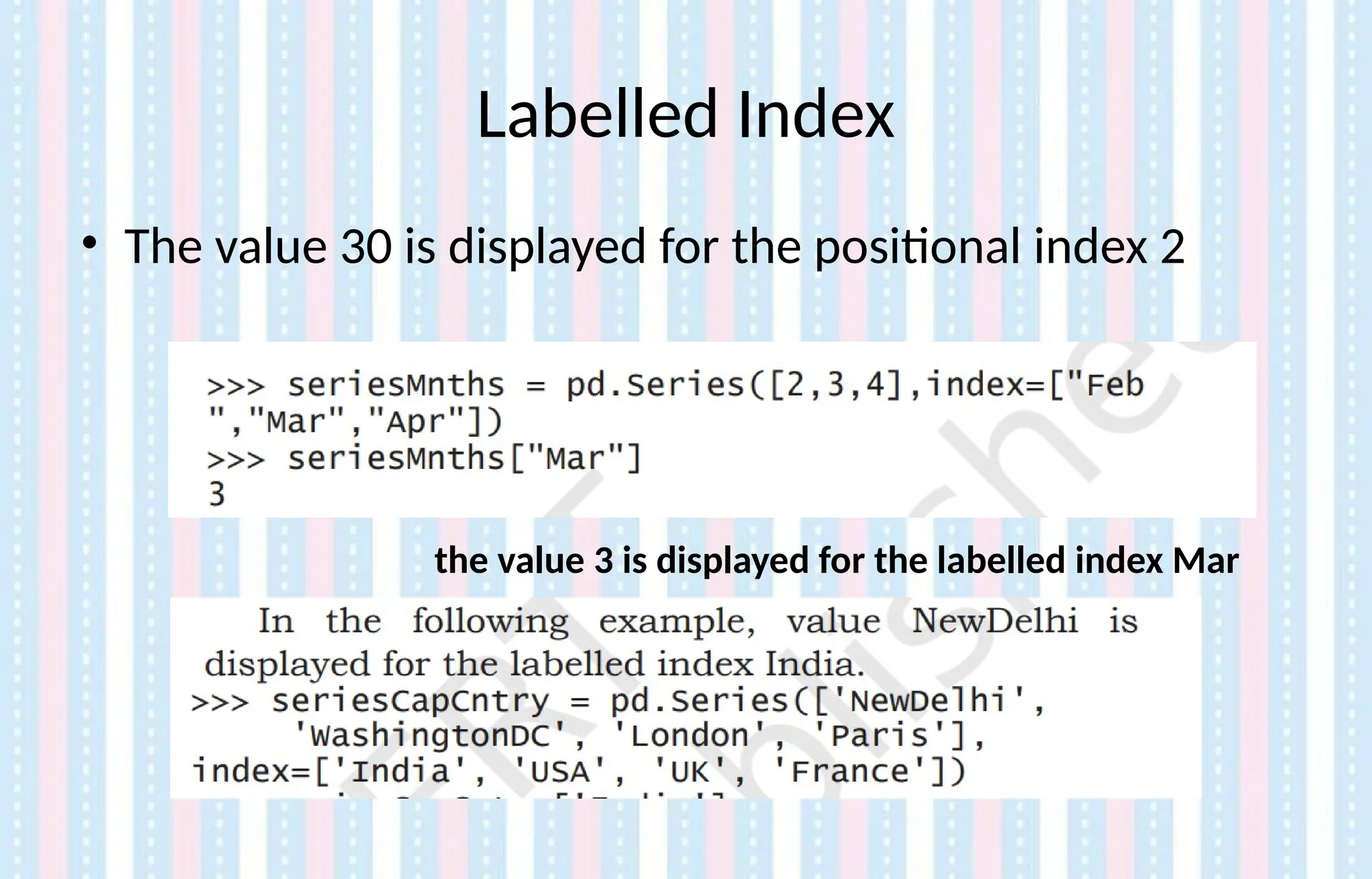
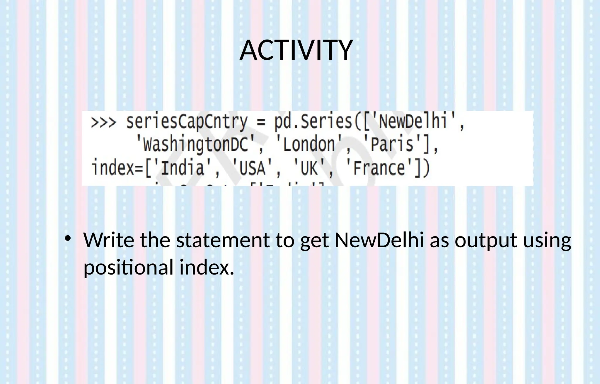
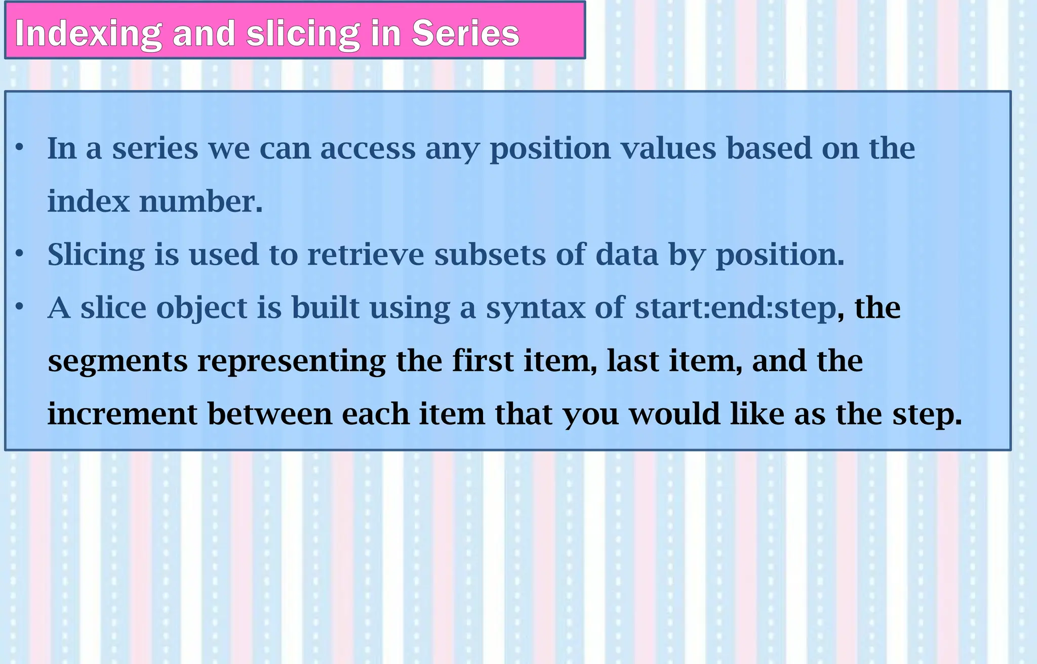
![Accessing Data from Series with indexing and slicing
import pandas aspd1
s = pd1.Series([1,2,3,4,5],index = ['a','b','c','d','e'])
>>> s[0]
1
>>> s[:3]
a 1
b 2
c 3
dtype: int64
>>> s[-3:]
c 3
d 4
e 5
dtype: int64](https://image.slidesharecdn.com/ln-250918173733-5ea4f2ca/75/Ln-1-Data-Handling-using-Pandas-I-1-pptx-70-2048.jpg)
![>>> fruits = ['apples', 'oranges', 'cherries', 'pears']
>>> S = pd.Series([20, 33, 52, 10], index=fruits)
>>> S
apples 20
oranges 33
cherries 52
pears 10
dtype: int64
>>> S['apples']
20
>>> S[0]
20
Accessing Data from Series with indexing and slicing](https://image.slidesharecdn.com/ln-250918173733-5ea4f2ca/75/Ln-1-Data-Handling-using-Pandas-I-1-pptx-71-2048.jpg)
![Find out the following-
AB
AB[2:4]
AB[1:6:2]
AB[ :6]
AB[4:]
AB[:4:2]
AB[4::2]
AB[::-1]
>>> num=[000,100,200,300,400,500,600,700,800,900]
>>> idx=['A','B','C','D','E','F','G','H','I','J']
>>> AB=pd.Series(num,index=idx)
Accessing Data from Series with indexing and slicing](https://image.slidesharecdn.com/ln-250918173733-5ea4f2ca/75/Ln-1-Data-Handling-using-Pandas-I-1-pptx-72-2048.jpg)
![Find out the following-
AB
AB[2:4]
AB[1:6:2]
AB[ :6]
AB[4:]
AB[:4:2] 0:4:2-- 000 200
AB[4::2] 400 600 800
AB[::-1]
>>> num=[000,100,200,300,400,500,600,700,800,900]
>>> idx=['A','B','C','D','E','F','G','H','I','J']
>>> AB=pd.Series(num,index=idx)
Accessing Data from Series with indexing and slicing](https://image.slidesharecdn.com/ln-250918173733-5ea4f2ca/75/Ln-1-Data-Handling-using-Pandas-I-1-pptx-73-2048.jpg)
![Create a series using 2 different lists
>>> import pandas as pd
>>> m=['jan','feb']
>>> n=[23,34]
>>> s=pd.Series(m,index=n)
>>> s
23 jan
34 feb
dtype: object](https://image.slidesharecdn.com/ln-250918173733-5ea4f2ca/75/Ln-1-Data-Handling-using-Pandas-I-1-pptx-74-2048.jpg)
![Printing the slices with the values of the label index
>>> M = pd.Series([400,500,345,450],index=['Amit','Raj','Kris','Shon'])
>>> M
Amit 400
Raj 500
Kris 345
Shon 450
dtype: int64
>>> M['Kris']
345
M[['Raj','Kris','Shon']]
Raj 500
Kris 345
Shon 450
dtype: int64
M['Raj':'Shon']
Raj 500
Kris 345
Shon 450
dtype: int64](https://image.slidesharecdn.com/ln-250918173733-5ea4f2ca/75/Ln-1-Data-Handling-using-Pandas-I-1-pptx-75-2048.jpg)
![Displaying the data using Boolean indexing
# Eg. To select marks more than 400
>>> M = pd.Series([400,500,345,450],index=['Amit','Raj','Kris','Shon'])
>>> M
Amit 400
Raj 500
Kris 345
Shon 450
dtype: int64
>>> M>400
Amit False
Raj True
Kris False
Shon True
dtype: bool
>>> M[M>400] #Will display the names of students who got marks >400
Raj 500
Shon 450
dtype: int64](https://image.slidesharecdn.com/ln-250918173733-5ea4f2ca/75/Ln-1-Data-Handling-using-Pandas-I-1-pptx-76-2048.jpg)
![Using range() to specify index in series
>>> S=pd.Series(5,index=range(4))
>>> S
0 5
1 5
2 5
3 5
dtype: int64
>>> S=pd.Series([1,2,3,4],index=range(4))
>>> S
0 1
1 2
2 3
3 4
dtype: int64](https://image.slidesharecdn.com/ln-250918173733-5ea4f2ca/75/Ln-1-Data-Handling-using-Pandas-I-1-pptx-77-2048.jpg)
![Using range() to specify index in series –for loop
>>> S=pd.Series(range(1,15,3),index=[x for i in ‘abcde’])
>>> S
a 1
b 4
c 7
d 10
e 13
dtype: int64
>>> S=pd.Series([1,2,3,4.0],index=range(4))
>>> S
0 1.0
1 2.0
2 3.0
3 4.0
dtype: float64](https://image.slidesharecdn.com/ln-250918173733-5ea4f2ca/75/Ln-1-Data-Handling-using-Pandas-I-1-pptx-78-2048.jpg)
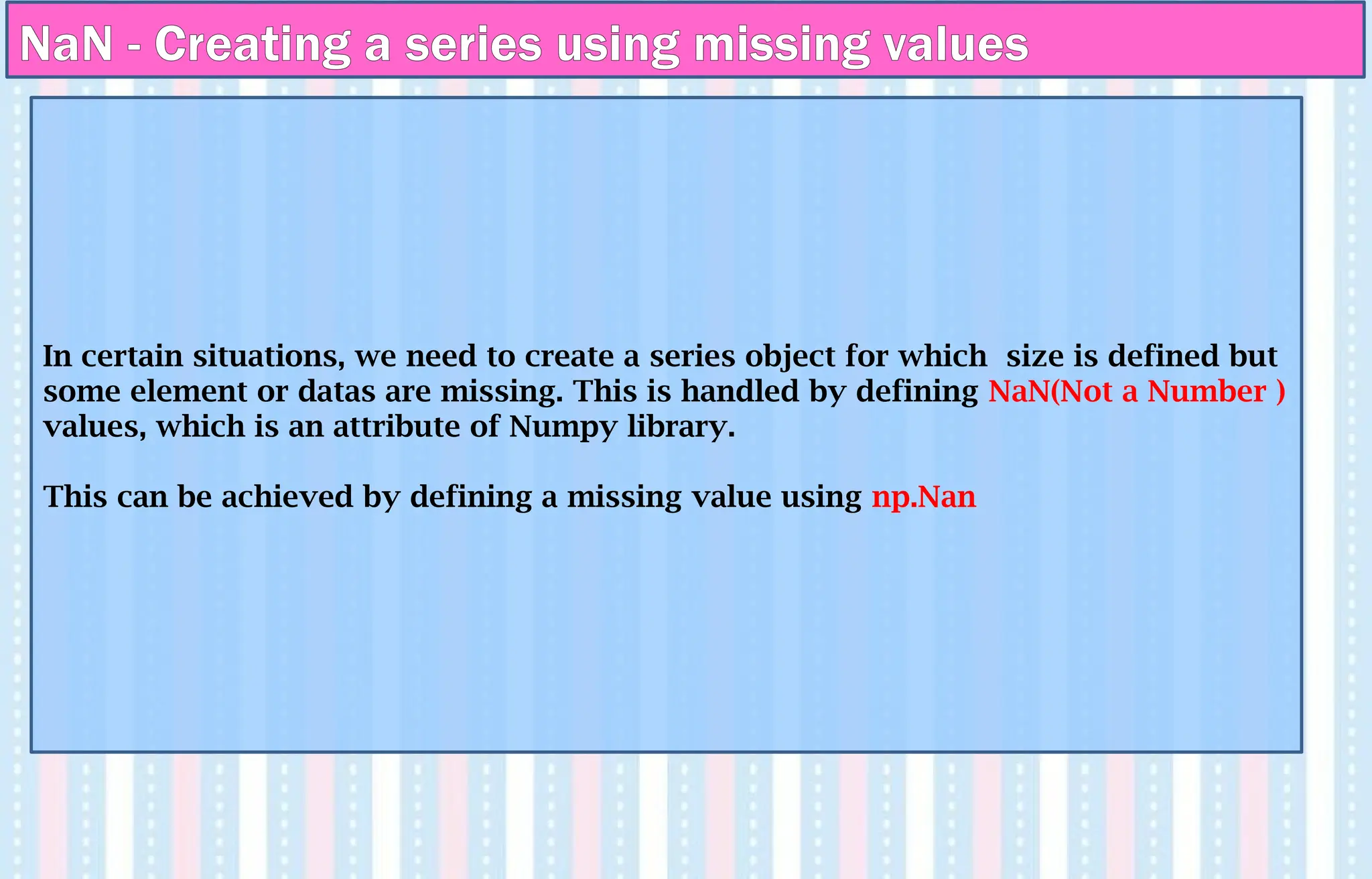
![NaN - Creating a series using missing values
Import pandas as pd
Import numpy as np
data = pd.Series([1, np.nan, 2, None, 3],
index= ('abcde'))
>>> data
a 1.0
b NaN
c 2.0
d NaN
e 3.0
dtype: float64
>>> d3=pd.Series(d1,index=[20,30,40,50,60])
>>> d3
20 NaN
30 NaN
40 NaN
50 NaN
60 NaN
dtype: float64
>>> s = pd.Series(np.nan, index=[49,3, 4, 5])
>>> s
49 NaN
3 NaN
4 NaN
5 NaN
dtype: float64](https://image.slidesharecdn.com/ln-250918173733-5ea4f2ca/75/Ln-1-Data-Handling-using-Pandas-I-1-pptx-80-2048.jpg)
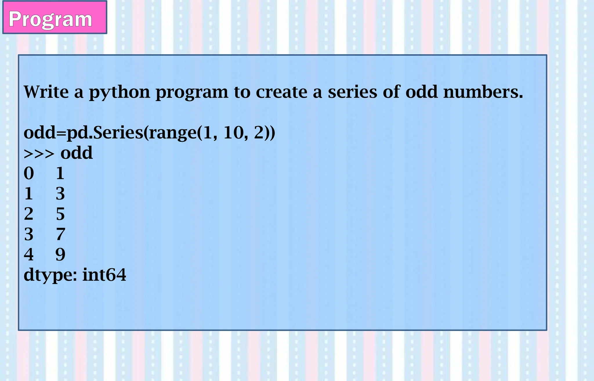

![CREATING SERIES WITH RANGE AND FOR LOOP
>>> S=pd.Series(range(1,15,3),index=[x for x in 'abcde'])
>>> S
a 1
b 4
c 7
d 10
e 13
dtype: int64](https://image.slidesharecdn.com/ln-250918173733-5ea4f2ca/75/Ln-1-Data-Handling-using-Pandas-I-1-pptx-83-2048.jpg)
![Handling floating point values to generate a series
import pandas as pd
ab=pd.Series([2,4,6,7.5])
ab
0 2.0
1 4.0
2 6.0
3 7.5
Dtype : float64
Since 7.5 is a float value, it will convert the rest of the integer
values to float and so it be overall a float series.](https://image.slidesharecdn.com/ln-250918173733-5ea4f2ca/75/Ln-1-Data-Handling-using-Pandas-I-1-pptx-84-2048.jpg)
![Indexing and accessing can also be done using iloc and loc.
iloc- It is used for indexing or selecting based on position ie..
By row number and column number. It refers to position
based indexing.
Syntax is-
iloc=[<row number range>,<col number range>]
loc – It is used to index or select based on name ie.. By row
name and col name. It refers to name based indexing.
Syntax is-
loc=[<list of row name>,<list of col name>]
So, we can filter the data using the loc function in Pandas even
if the indices are not an integer in our dataset.
Note- By default, index is assigned from 0 to len-1.
iloc and loc](https://image.slidesharecdn.com/ln-250918173733-5ea4f2ca/75/Ln-1-Data-Handling-using-Pandas-I-1-pptx-85-2048.jpg)
![import pandas as pd
a=pd.Series([1,2,3,4,5], index=‘a’,’b’,’c’,’d’,’e’])
>>> a.iloc[1:4] # Displays data using index
b 2
c 3
d 4
dtype: int64
>>> a.loc['b':'e'] # Displays data location wise
b 2
c 3
d 4
e 5
dtype: int64
loc and iloc](https://image.slidesharecdn.com/ln-250918173733-5ea4f2ca/75/Ln-1-Data-Handling-using-Pandas-I-1-pptx-86-2048.jpg)
![>>> s = pd.Series(np.nan, index=[49,48,47,46,45, 1, 2, 3, 4, 5])
>>> s.iloc[:3] # slice the first three rows
49 NaN
48 NaN
47 NaN
>>> s.loc[:3] # slice up to and including label 3
49 NaN
48 NaN
47 NaN
46 NaN
45 NaN
1 NaN
2 NaN
3 NaN
loc and iloc](https://image.slidesharecdn.com/ln-250918173733-5ea4f2ca/75/Ln-1-Data-Handling-using-Pandas-I-1-pptx-87-2048.jpg)
![loc vs. iloc in Pandas
loc
• Purely label-location based indexer for selection by label.
• It is primarily label based, but may also be used with a
boolean array.
• Allowed inputs are:
A single label, e.g. 5 or 'a'.
A list or array of labels, e.g. ['a', 'b', 'c'].
A slice object with labels, e.g. 'a':'f' (note that contrary to usual
python slices, both the start and the stop are included!).
A boolean array.
A callable function with one argument (the calling Series,
DataFrame ) and that returns valid output for indexing (one of
the above)
• Note : .loc will raise a KeyError when the items are not
found](https://image.slidesharecdn.com/ln-250918173733-5ea4f2ca/75/Ln-1-Data-Handling-using-Pandas-I-1-pptx-88-2048.jpg)
![iloc-
• .iloc is primarily integer position based (from 0 to length-
1 of the axis), but may also be used with a boolean array.
• .iloc will raise IndexError if a requested indexer is out-of-
bounds, except slice indexers which allow out-of-bounds
indexing.
• Allowed inputs are:
An integer e.g. 5
A list or array of integers [4, 3, 0]
A slice object with ints 1:7
A boolean array
A callable function with one argument
loc vs. iloc in Pandas](https://image.slidesharecdn.com/ln-250918173733-5ea4f2ca/75/Ln-1-Data-Handling-using-Pandas-I-1-pptx-89-2048.jpg)
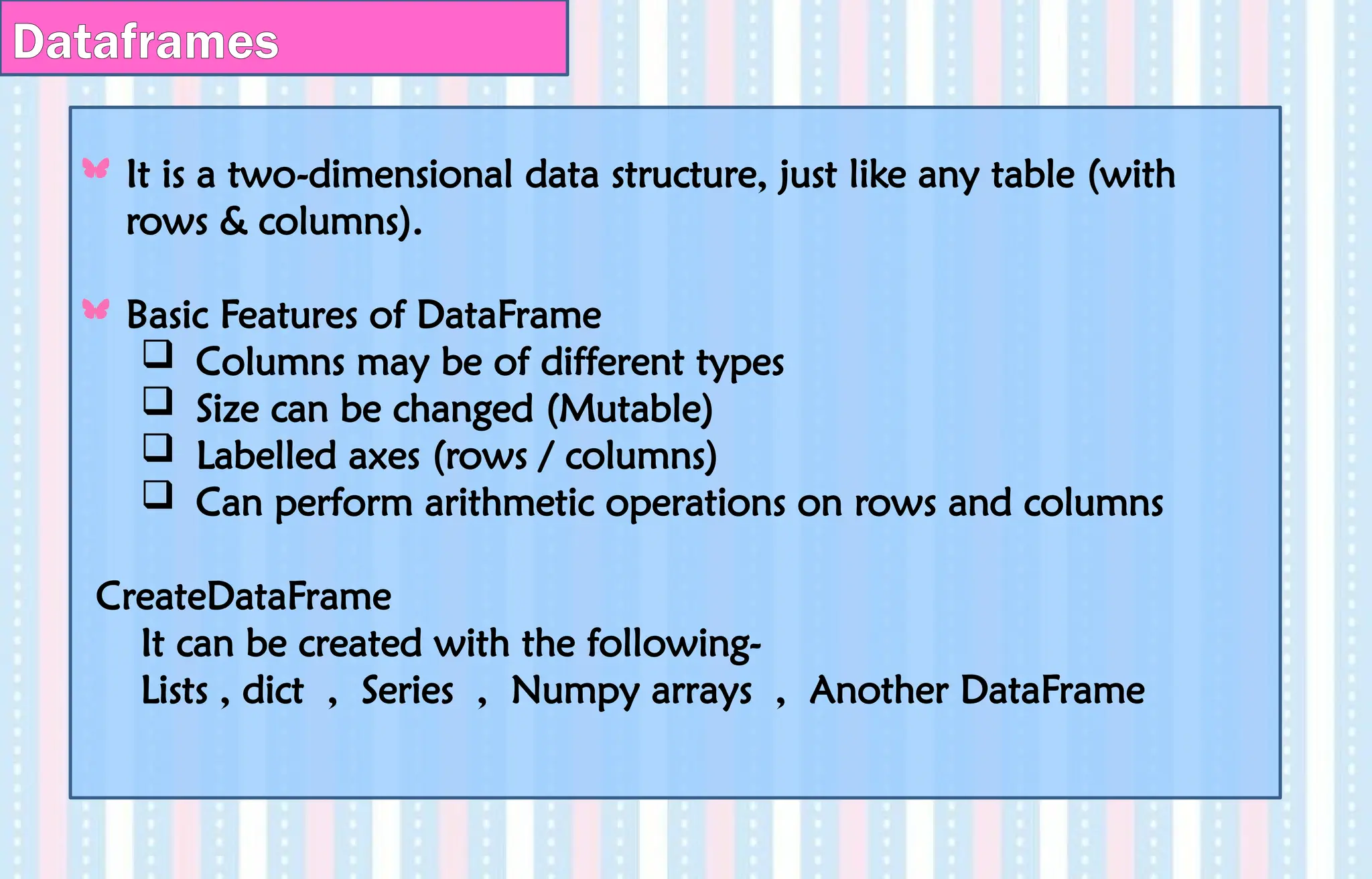
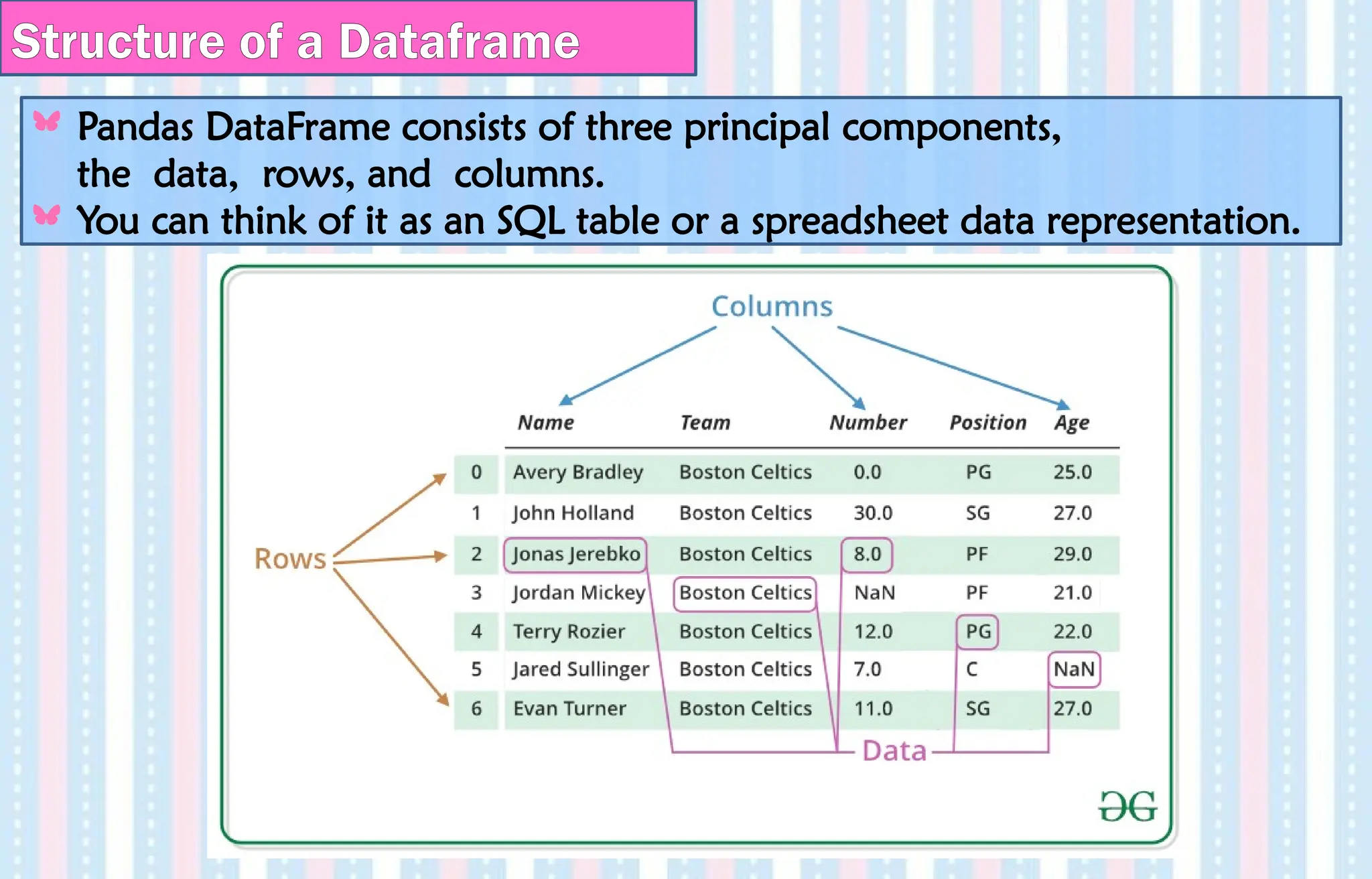
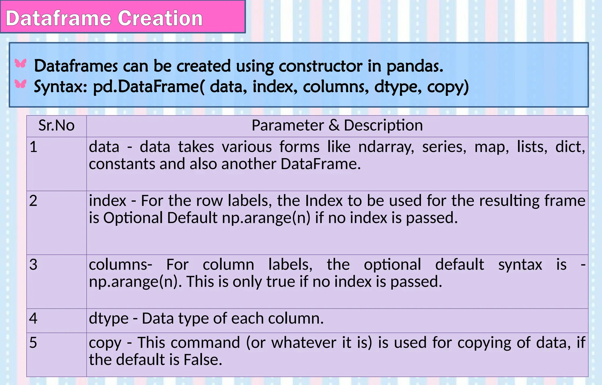
![Creating an empty Dataframe
A basic DataFrame, which can be created is an Empty Dataframe.
>>> import pandas as pd
>>> d=pd.DataFrame()
>>> d
Empty DataFrame
Columns: []
Index: []](https://image.slidesharecdn.com/ln-250918173733-5ea4f2ca/75/Ln-1-Data-Handling-using-Pandas-I-1-pptx-93-2048.jpg)
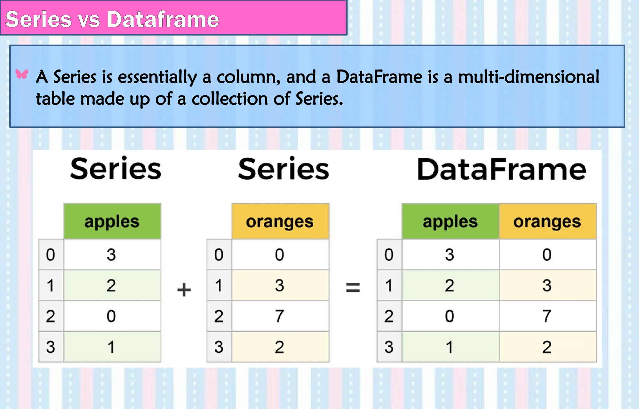
![Creating a Dataframe from lists with values only
The DataFrame can be created using a single list or a list of lists.
CREATING A DATAFRAME FROM SINGLE LIST
Example1:
import pandas as pd
data = [1,2,3,4,5]
df = pd.DataFrame(data)
print (df)](https://image.slidesharecdn.com/ln-250918173733-5ea4f2ca/75/Ln-1-Data-Handling-using-Pandas-I-1-pptx-95-2048.jpg)
![Creating a Dataframe from lists of lists (multidimensional list)
CREATE A DATAFRAME FROM A LIST OF LISTS
import pandas as pd
data = [['Alex',10],['Bob',12],['Clarke',13]]
df = pd.DataFrame(data,columns=['Name','Age'])
print (df)
Name Age
0 Alex 10
1 Bob 12
2 Clarke 13](https://image.slidesharecdn.com/ln-250918173733-5ea4f2ca/75/Ln-1-Data-Handling-using-Pandas-I-1-pptx-96-2048.jpg)
![Creating a Dataframe from lists of lists (multidimensional list)
import pandas as pd
>>> a=[12,13,14,15]
>>> b=[20,30,40,50]
>>> c=pd.DataFrame(a,index=[b],columns=['Numbers'],dtype='float')
>>> c
Numbers
20 12.0
30 13.0
40 14.0
50 15.0](https://image.slidesharecdn.com/ln-250918173733-5ea4f2ca/75/Ln-1-Data-Handling-using-Pandas-I-1-pptx-97-2048.jpg)
![Example
>>> data = [[0, 1, 2],[3, 4, 5]]
>>> df = pd.DataFrame(data)
>>> df
0 1 2
0 0 1 2
1 3 4 5](https://image.slidesharecdn.com/ln-250918173733-5ea4f2ca/75/Ln-1-Data-Handling-using-Pandas-I-1-pptx-98-2048.jpg)
![Creating a Dataframe from lists of lists (multidimensional list)
Using multi-dimensional list with column name and dtype
specified.
import pandas as pd
lst = [['tom', 'reacher', 25], ['krish', 'pete', 30],
['nick', 'wilson', 26], ['juli', 'williams', 22]]
df = pd.DataFrame(lst, columns =['FName', 'LName', 'Age'],
dtype = float)
df](https://image.slidesharecdn.com/ln-250918173733-5ea4f2ca/75/Ln-1-Data-Handling-using-Pandas-I-1-pptx-99-2048.jpg)
![Program
Display the following details in a dataframe.
Name Marks Index
Vijaya 80 B1
Rahul 92 A2
Meghna 67 C
Radhika 95 A1
Shaurya 97 A1
df = pd.DataFrame(lst, columns =['FName', 'LName', 'Age'], dtype = float)](https://image.slidesharecdn.com/ln-250918173733-5ea4f2ca/75/Ln-1-Data-Handling-using-Pandas-I-1-pptx-100-2048.jpg)
![Displaying index and col
>>> df = pd.DataFrame([[0, 1, 2], [3, 4, 5]], index=['row1',
'row2'],columns=['col1', 'col2', 'col3'])
>>> df
col1 col2 col3
row1 0 1 2
row2 3 4 5
>>> print(df.index)
Index(['row1', 'row2'], dtype='object')
>>> print(df.columns)
Index(['col1', 'col2', 'col3'], dtype='object')](https://image.slidesharecdn.com/ln-250918173733-5ea4f2ca/75/Ln-1-Data-Handling-using-Pandas-I-1-pptx-101-2048.jpg)
![Creating DataFrames from Series
DataFrames are 2 dimensional representation of Series.
When we represent 2 or more series in the form of rows and columns,
it becomes a dataframe.
Lets create 2 series and pass it into a dataframe.
>>> p={'one':pd.Series([1,2,3], index=['a','b','c']), 'two':pd.Series
([11,22,33,44], index=['a','b','c','d'])}
>>> q=pd.DataFrame(p)
>>> q
one two
a 1.0 11
b 2.0 22
c 3.0 33
d NaN 44](https://image.slidesharecdn.com/ln-250918173733-5ea4f2ca/75/Ln-1-Data-Handling-using-Pandas-I-1-pptx-102-2048.jpg)
![>>> p=pd.Series([10,20,30],index=['a','b','c'])
>>> q=pd.Series([40,50,60],index=['a','b','c'])
>>> r=pd.DataFrame({'Set1':p , 'Set2':q})
>>> r
Set1 Set2
a 10 40
b 20 50
c 30 60
Creating DataFrames from Series](https://image.slidesharecdn.com/ln-250918173733-5ea4f2ca/75/Ln-1-Data-Handling-using-Pandas-I-1-pptx-103-2048.jpg)
![Creating DataFrames from Series
# To create dataframe from 2 series of student data
import pandas as pd
stud_marks=pd.Series([89,94,93,83,89],index=['Anuj','Deepak','Sohail'
,'Tresa','Hima'])
stud_age=pd.Series([18,17,19,16,18],index=['Anuj','Deepak','Sohail','Tre
sa','Hima'])
>>> stud=pd.DataFrame({'Marks':stud_marks,'Age':stud_age})
>>> stud
Marks Age
Anuj 89 18
Deepak 94 17
Sohail 93 19
Tresa 83 16
Hima 89 18](https://image.slidesharecdn.com/ln-250918173733-5ea4f2ca/75/Ln-1-Data-Handling-using-Pandas-I-1-pptx-104-2048.jpg)
![Sorting data in DataFrames
We can sort the data inside a dataframe using sort_values().
Here 2 arguments are passed- sorting field and the order of sorting (asc
or desc).
‘By’ keyword, defines the name of the field or column based on which
it is to be sorted.
>>> stud.sort_values(by=['Marks'])
Marks Age
Tresa 83 16
Anuj 89 18
Hima 89 18
Sohail 93 19
Deepak 94 17
stud.sort_values(by=['Marks'],ascending=False)
Marks Age
Deepak 94 17
Sohail 93 19
Anuj 89 18
Hima 89 18
Tresa 83 16](https://image.slidesharecdn.com/ln-250918173733-5ea4f2ca/75/Ln-1-Data-Handling-using-Pandas-I-1-pptx-105-2048.jpg)
![Creating DataFrame from Dictionary (Dictionary of Lists)
• List of dictionaries can be passed as an input data to create a dataframe.
• The dictionary keys are by default, taken as column names.
import pandas as pd
data = {'Name':['Tom', 'Jack', 'Steve', 'Ricky'],'Age':[28,34,29,42]}
df = pd.DataFrame(data)
print (df)
Age Name
0 28 Tom
1 34 Jack
2 29 Steve
3 42 Ricky](https://image.slidesharecdn.com/ln-250918173733-5ea4f2ca/75/Ln-1-Data-Handling-using-Pandas-I-1-pptx-106-2048.jpg)
![Program
cars = {'Brand': ['Honda Civic','Toyota Corolla','Ford Focus','Audi A4'],
'Price': [22000,25000,27000,35000] }
df = pd.DataFrame(cars, columns = ['Brand', 'Price'])
print (df)
Brand Price
0 Honda Civic 22000
1 Toyota Corolla 25000
2 Ford Focus 27000
3 Audi A4 35000
Brand Price
car1 Honda Civic 22000
car2 Toyota Corolla 25000
car3 Ford Focus 27000
car4 Audi A4 35000](https://image.slidesharecdn.com/ln-250918173733-5ea4f2ca/75/Ln-1-Data-Handling-using-Pandas-I-1-pptx-107-2048.jpg)
![import pandas as pd
data = { ‘Name ‘ : [ ‘Tom’,’Jack’,’Steve’,’Ricky’], ‘Age’ : [28,34,29,42] }
df = pd.DataFrame (data, index = [‘rank 1’, ‘rank 2’, ‘rank 3’, ‘rank 4’ ])
print ( df )
output
AGE NAME
RANK 1 28 tOM
RANK 2 34 jACK
RANK 3 29 Steve
RANK 4 42 Ricky
Program - Create an indexed DataFrame](https://image.slidesharecdn.com/ln-250918173733-5ea4f2ca/75/Ln-1-Data-Handling-using-Pandas-I-1-pptx-108-2048.jpg)
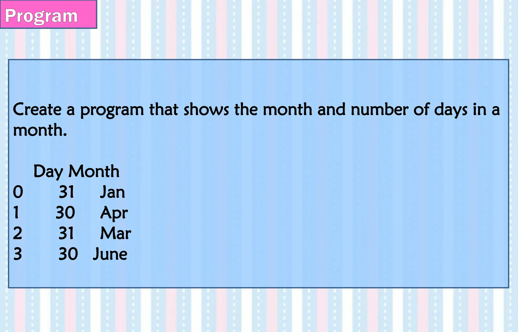
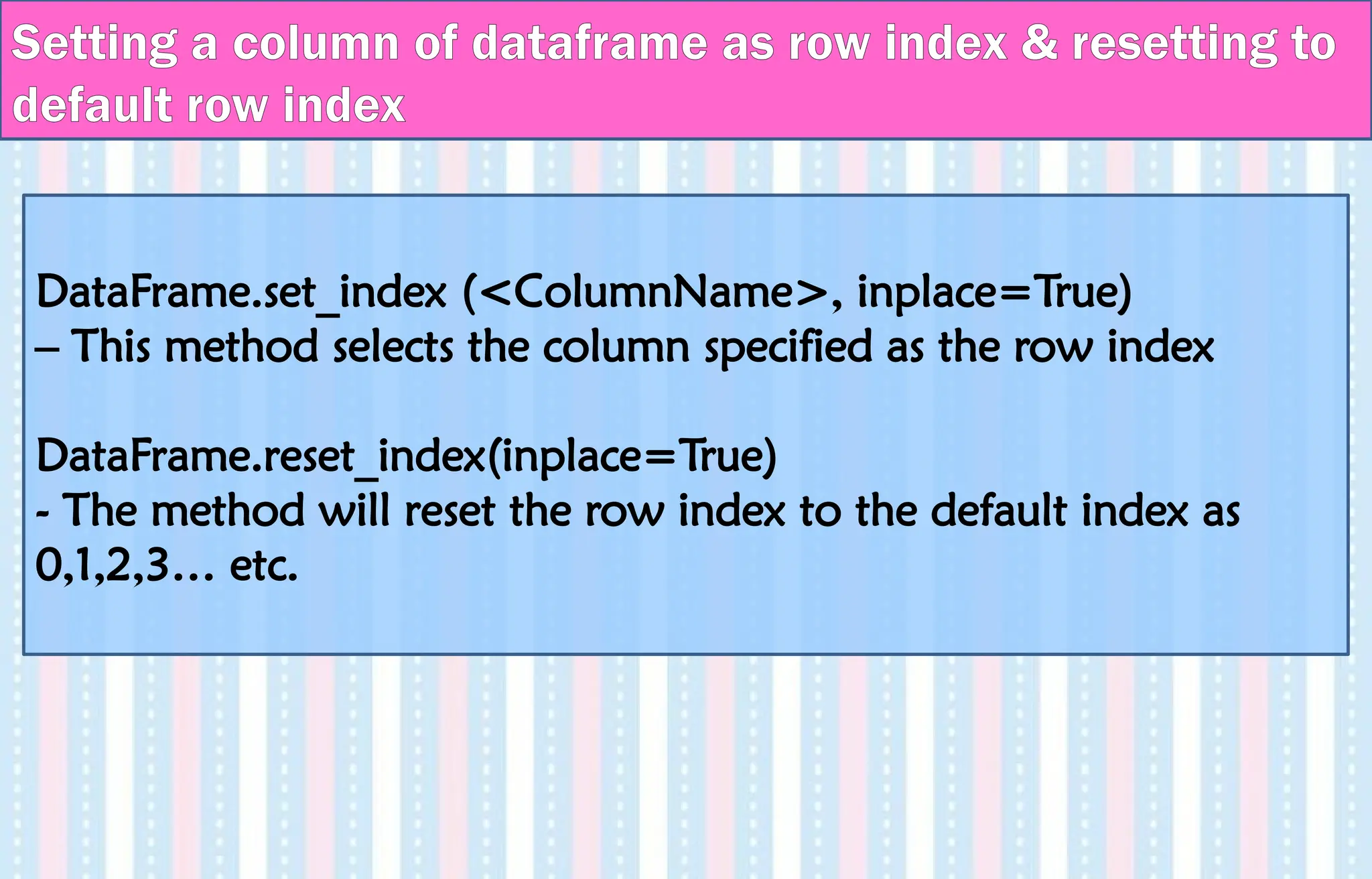
![Suppose we want to make one of the columns as row index:
import pandas as pd
data = {'Name':['Tom', 'Jack', 'Steve', 'Ricky'],'Age':[28,34,29,42]}
df = pd.DataFrame(data)
df.set_index('Name',inplace=True)
print (df)
Age
Name
Tom 28
Jack 34
Steve 29
Ricky 42
Example](https://image.slidesharecdn.com/ln-250918173733-5ea4f2ca/75/Ln-1-Data-Handling-using-Pandas-I-1-pptx-111-2048.jpg)
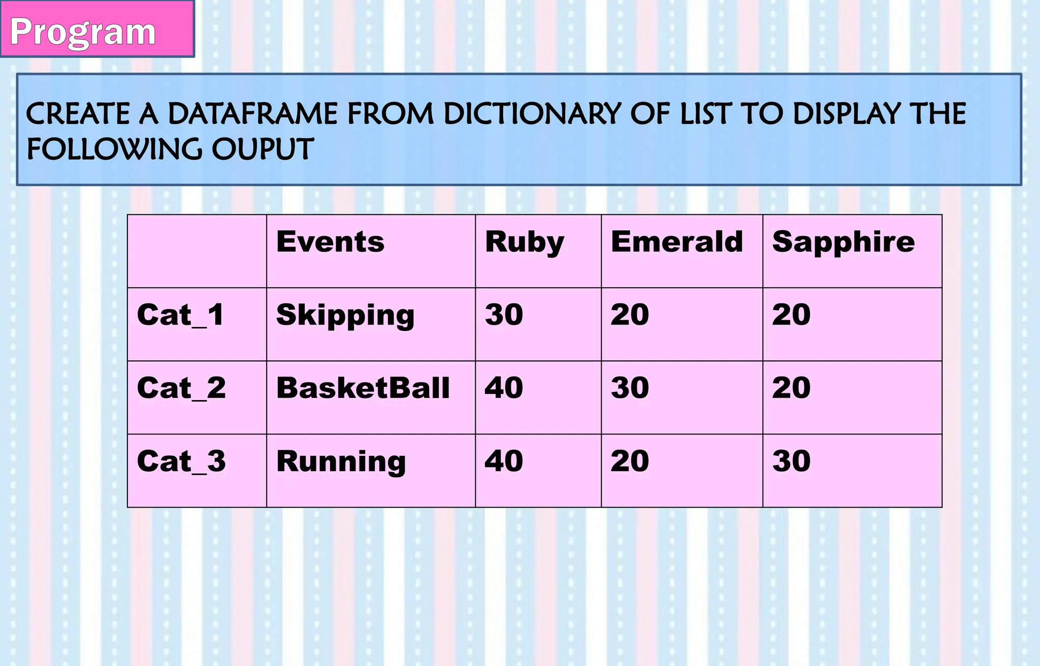
![# Create a DataFrame from List of Dictionaries
import pandas as pd
data1 = [{'x': 1, 'y': 2},{'x': 5, 'y': 4, 'z':5}]
df1 =pd.DataFrame(data1)
x y z
0 1 2 NaN
1 5 4 5.0
Note − Observe, NaN (Not a Number) is appended in missing
areas.
Program](https://image.slidesharecdn.com/ln-250918173733-5ea4f2ca/75/Ln-1-Data-Handling-using-Pandas-I-1-pptx-113-2048.jpg)
![Create a DataFrame with a list of dictionaries, row indices, and
column indices.
import pandas as pd
data = [{'a': 1, 'b': 2},{'a': 5, 'b': 10, 'c': 20}]
df1 = pd.DataFrame(data, index=['first', 'second'], columns=['a',
'b‘,’c’])
>>> df1
a b c
first 1 2 NaN
second 5 10 20.0
Program](https://image.slidesharecdn.com/ln-250918173733-5ea4f2ca/75/Ln-1-Data-Handling-using-Pandas-I-1-pptx-114-2048.jpg)
![ Create a series from a one list containing authors name and another list
containing number of articles written.
Create a dataframe from the series created using a dictionary containing key as
“Authors” and “Articles”
The following output must be obtained:
Program
import pandas as pd
a=["Jitender","Purnima","Arpit","Jyoti"]
b=[210,211,114,178]
s = pd.Series(a)
s1= pd.Series(b)
df=pd.DataFrame({"Author":s,"Article":s1})
df](https://image.slidesharecdn.com/ln-250918173733-5ea4f2ca/75/Ln-1-Data-Handling-using-Pandas-I-1-pptx-115-2048.jpg)
![• To access and retrieve the records from a dataframe, we need to use slice
operation.
• Slicing will display the retrieved records as per the defined range.
import pandas as pd
student={'Name':['Rinku','Ritu','Ajay','Pankaj','Aditya'], 'English':[84,56,89,
78,36], 'Economics':[96,56,89,45,95], 'IP':[83,85,88,92,97], 'Accounts':
[77,75,63,89,85]}
>>> df=pd.DataFrame(student)
>>> df
Name English Economics IP Accounts
0 Rinku 84 96 83 77
1 Ritu 56 56 85 75
2 Ajay 89 89 88 63
3 Pankaj 78 45 92 89
4 Aditya 36 95 97 85
Selecting & Accessing from DataFrame](https://image.slidesharecdn.com/ln-250918173733-5ea4f2ca/75/Ln-1-Data-Handling-using-Pandas-I-1-pptx-116-2048.jpg)
![df[1:4] # Records from 1st
to 3rd
row are displayed
Name English Economics IP Accounts
1 Ritu 56 56 85 75
2 Ajay 89 89 88 63
3 Pankaj 78 45 92 89
Note- Single row accessing is not possible.
To display a whole column,
>>> df['Name']
To display more than 1 columns,
>>> df[['Name','IP']]
>>> df['Name'][0:3]
0 Rinku
1 Ritu
2 Ajay
Name: Name, dtype: object
Selecting & Accessing from DataFrame](https://image.slidesharecdn.com/ln-250918173733-5ea4f2ca/75/Ln-1-Data-Handling-using-Pandas-I-1-pptx-117-2048.jpg)
![• Pandas provides us the flexibility to even change or rename any column inside a
dataframe.
• To change for a single column-
df.rename(columns={'Name':'Emp_Name'}, inplace=True)
• Consider a list of age of students-
a1=[20,30,25,26,15]
Rename the column ‘a1’ to ‘age’
>>> a1=[20,30,25,26,15]
>>> a1
[20, 30, 25, 26, 15]
Renaming column in DataFrame
>>> df=pd.DataFrame(a1)
>>> df
0
0 20
1 30
2 25
3 26
4 15
>>> df.columns=['Age']
>>> df
Age
0 20
1 30
2 25
3 26
4 15](https://image.slidesharecdn.com/ln-250918173733-5ea4f2ca/75/Ln-1-Data-Handling-using-Pandas-I-1-pptx-118-2048.jpg)
![• To add new columns to an already existing dataframe, the syntax is-
dfobject.colname[row_label]=new_value
>>> df['Age1']=45 # the entire column is filled up with 45
>>> df
Age Age1
0 20 45
1 30 45
2 25 45
3 26 45
4 15 45
Adding column to a DataFrame
df['Age3']=pd.Series([42,35,44,50,60])
df
Age Age2 Age3
0 20 45 42
1 30 45 35
2 25 45 44
3 26 45 50
4 15 45 60
df['Total']=df['Age']+df['Age2']+df['Age3']
df
Age Age2 Age3 Total
0 20 45 42 107
1 30 45 35 110
2 25 45 44 114
3 26 45 50 121
4 15 45 60 120](https://image.slidesharecdn.com/ln-250918173733-5ea4f2ca/75/Ln-1-Data-Handling-using-Pandas-I-1-pptx-119-2048.jpg)
![• We can update a column values by using arithmetic operators.
• We can also assign or copy the values of a dataframe with the help of assignment
operator.
• To add a new column for updated_age after 10 years for all students,
>>> df['Total']=df['Total']+10
>>> df
Age Age2 Age3 Total
0 20 45 42 117
1 30 45 35 120
2 25 45 44 124
3 26 45 50 131
4 15 45 60 130
>>> df['Updated_Age']=df['Total']
>>> df
Age Age2 Age3 Total Updated_Age
0 20 45 42 117 117
1 30 45 35 120 120
2 25 45 44 124 124
3 26 45 50 131 131
4 15 45 60 130 130
Adding column to a DataFrame](https://image.slidesharecdn.com/ln-250918173733-5ea4f2ca/75/Ln-1-Data-Handling-using-Pandas-I-1-pptx-120-2048.jpg)
![1. Create a dataframe from the dictionary of list.
Name Height Qualification
0 Jai 5.1 Msc
1 Princi 6.2 MA
2 Gaurav 5.1 Msc
3 Anuj 5.2 Msc
2. Add a column address to the dataframe with values:
address = ['Delhi', 'Bangalore', 'Chennai', 'Patna']
Sample Question-](https://image.slidesharecdn.com/ln-250918173733-5ea4f2ca/75/Ln-1-Data-Handling-using-Pandas-I-1-pptx-121-2048.jpg)
![data = {'Name': ['Jai', 'Princi', 'Gaurav', 'Anuj'],'Height': [5.1, 6.2, 5.1,
5.2],'Qualification': ['Msc', 'MA', 'Msc', 'Msc']}
df = pd.DataFrame(data)
>>> df['address']=['Delhi', 'Bangalore', 'Chennai', 'Patna']
>>> df
Name Height Qualification address
0 Jai 5.1 Msc Delhi
1 Princi 6.2 MA Bangalore
2 Gaurav 5.1 Msc Chennai
3 Anuj 5.2 Msc Patna
Sample Question-](https://image.slidesharecdn.com/ln-250918173733-5ea4f2ca/75/Ln-1-Data-Handling-using-Pandas-I-1-pptx-122-2048.jpg)
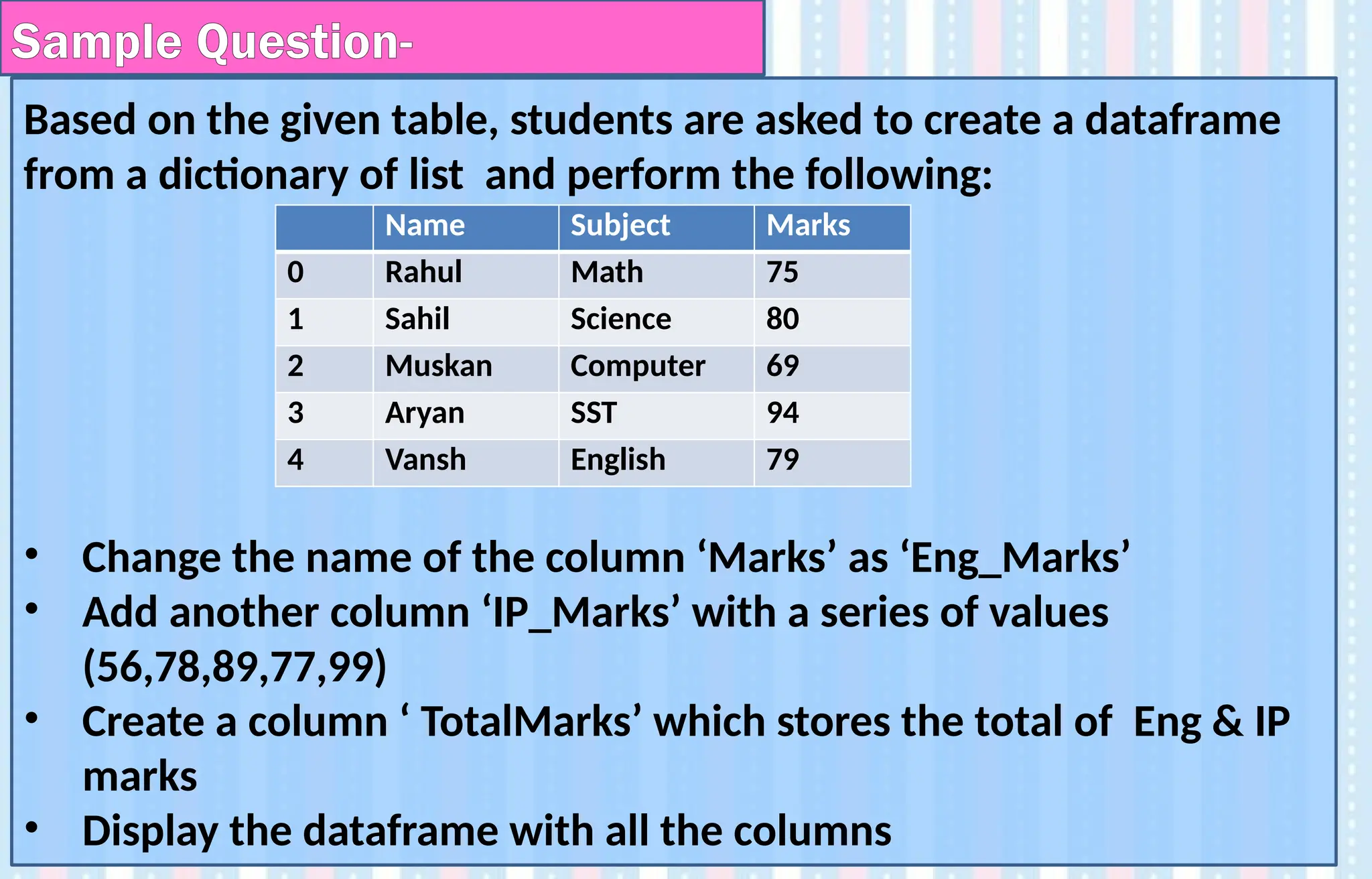

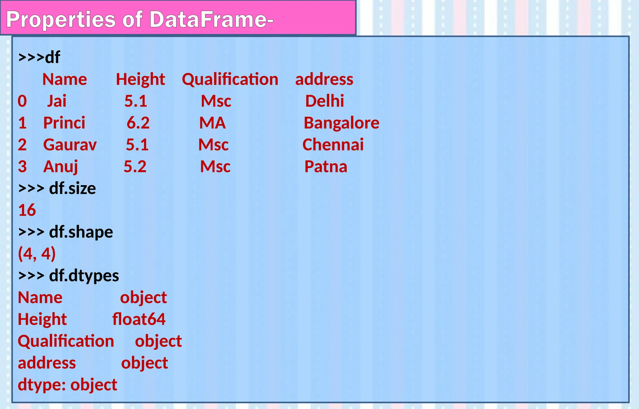
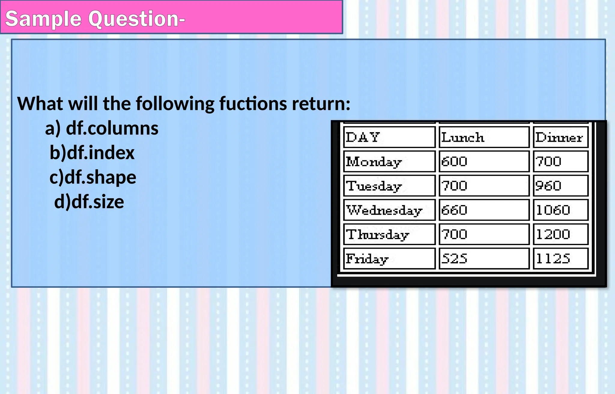
![import pandas as pd
df = pd.DataFrame({'Date':['10/2/2011', '11/2/2011', '12/2/2011',
'13/2/11'], 'Event':['Music', 'Poetry', 'Theatre', 'Comedy'], 'Cost':
[10000, 5000, 15000, 2000]})
print (df)
print(df.index)
print(df.columns)
print(df.dtype)
print(df.size)
print(df.shape)
Sample Question-](https://image.slidesharecdn.com/ln-250918173733-5ea4f2ca/75/Ln-1-Data-Handling-using-Pandas-I-1-pptx-127-2048.jpg)
![• The method of selecting / accessing a column of a dataframe is
similar to slicing using series.
• Pandas provides 3 methods to access dataframe column(s)
Using the format of square brackets followed by the name of the
column passed as a string value, like
df_object.[‘column_name’]
Using the dot notation df_object.column_name
Using numeric indexing and the iloc attribute, like
df_object.iloc[:,<column_number>]
• Here , i stands for integer, which signifies that this command shall
return a numeric value denoting the row and column range
SELECTING A COLUMN FROM A DATAFRAME](https://image.slidesharecdn.com/ln-250918173733-5ea4f2ca/75/Ln-1-Data-Handling-using-Pandas-I-1-pptx-128-2048.jpg)
![• Example-
df[‘Total’] and df.Total will give the same output.
SELECTING A COLUMN FROM A DATAFRAME](https://image.slidesharecdn.com/ln-250918173733-5ea4f2ca/75/Ln-1-Data-Handling-using-Pandas-I-1-pptx-129-2048.jpg)
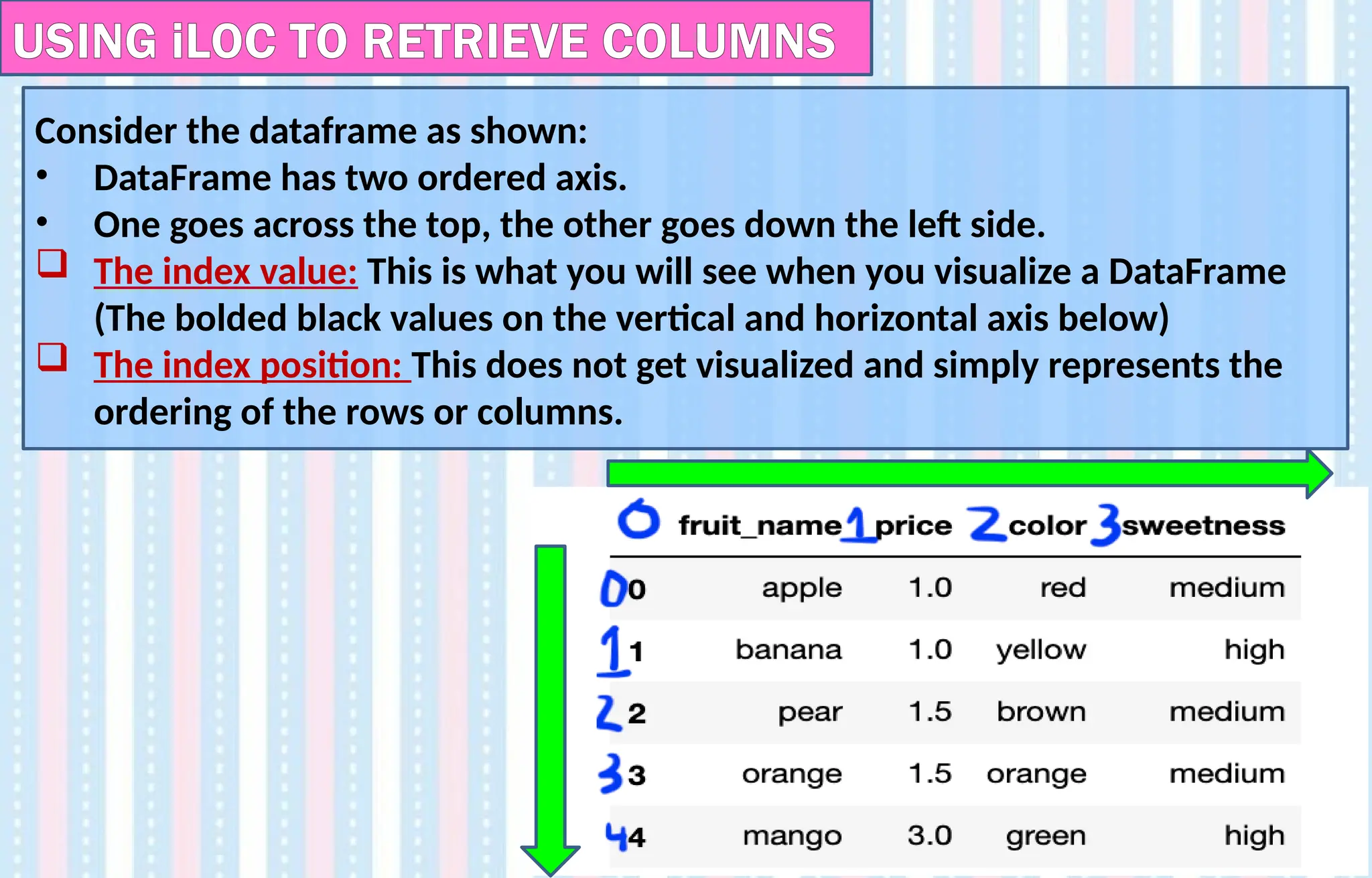
![USING iLOC TO RETRIEVE COLUMNS
Vertical Index Values: [0, 1, 2, 3, 4]
Vertical Index Positions: [0, 1, 2, 3, 4]
Horizontal Index Values: [‘fruit_name’, ‘price, ‘color’, ‘sweetness’]
Horizontal Index Positions: [0, 1, 2, 3]](https://image.slidesharecdn.com/ln-250918173733-5ea4f2ca/75/Ln-1-Data-Handling-using-Pandas-I-1-pptx-131-2048.jpg)
![USING iLOC TO RETRIEVE COLUMNS
iloc allows us to index a DataFrame in the same way that we
can index a list; based on index position.
The difference is that a DataFrame has a two-dimensional
index, so we need to pass in slicers for the rows first and
then for the columns.
There are four 4 possible types of slicers we can use on the
table given:
• Scalar positions (eg:- 0,3,4)
• Range of positions (eg:- 0:1, 1:4)
• All positions (:)
• List of positions (eg:- [0,3] , [1,5])](https://image.slidesharecdn.com/ln-250918173733-5ea4f2ca/75/Ln-1-Data-Handling-using-Pandas-I-1-pptx-132-2048.jpg)
![If we want to select the data in row 2 and column 0 (i.e., row
index 2 and column index 0) we’ll use the following code:
df.iloc[2,0]
USING iloc- Integer locate](https://image.slidesharecdn.com/ln-250918173733-5ea4f2ca/75/Ln-1-Data-Handling-using-Pandas-I-1-pptx-133-2048.jpg)
![Example - USING iloc- Integer locate
>>> df = pd.DataFrame({'Date':['10/2/2011', '11/2/2011', '12/2/2011',
'13/2/11'], 'Event':['Music', 'Poetry', 'Theatre', 'Comedy'], 'Cost':[10000, 5000,
15000, 2000]})
>>> df
Date Event Cost
0 10/2/2011 Music 10000
1 11/2/2011 Poetry 5000
2 12/2/2011 Theatre 15000
3 13/2/11 Comedy 2000
>>> df.iloc[1,1]
'Poetry'
>>> df.iloc[-1,0]
'13/2/11'
>>> df.iloc[2,2]
15000](https://image.slidesharecdn.com/ln-250918173733-5ea4f2ca/75/Ln-1-Data-Handling-using-Pandas-I-1-pptx-134-2048.jpg)
![Example - USING iloc- Integer locate
>>> df = pd.DataFrame({'Date':['10/2/2011', '11/2/2011', '12/2/2011', '13/2/11'],
'Event':['Music', 'Poetry', 'Theatre', 'Comedy'], 'Cost':[10000, 5000, 15000, 2000]})
>>> df
Date Event Cost
0 10/2/2011 Music 10000
1 11/2/2011 Poetry 5000
2 12/2/2011 Theatre 15000
3 13/2/11 Comedy 2000
>>> df.iloc[2:4,0:3]
Date Event Cost
2 12/2/2011 Theatre 15000
3 13/2/11 Comedy 2000](https://image.slidesharecdn.com/ln-250918173733-5ea4f2ca/75/Ln-1-Data-Handling-using-Pandas-I-1-pptx-135-2048.jpg)
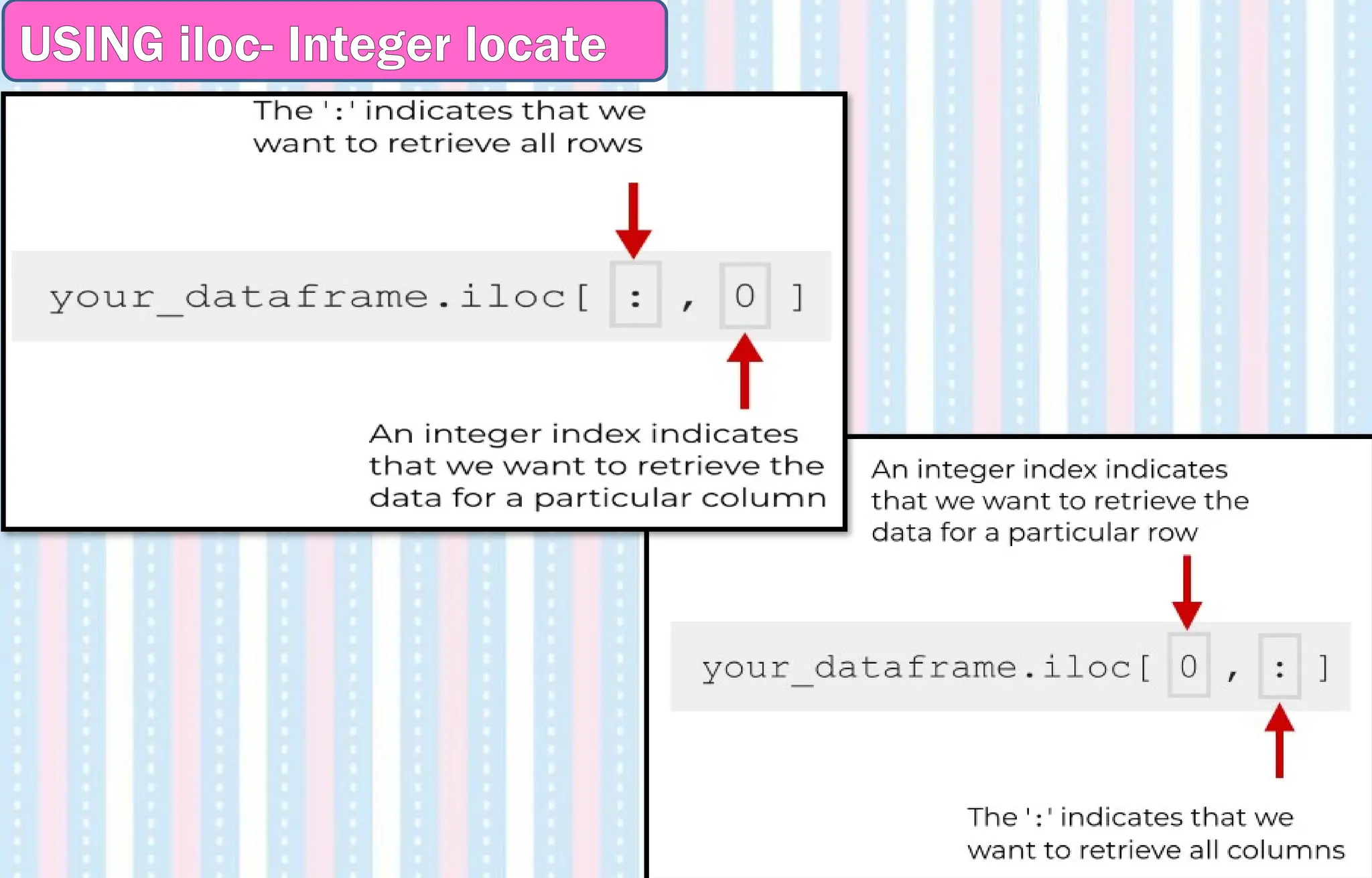

![Example - USING iloc- Integer locate
>>> df
>>> df
Date Event Cost
0 10/2/2011 Music 10000
1 11/2/2011 Poetry 5000
2 12/2/2011 Theatre 15000
3 13/2/11 Comedy 2000
>>> df.iloc[:,:]
Date Event Cost
0 10/2/2011 Music 10000
1 11/2/2011 Poetry 5000
2 12/2/2011 Theatre 15000
3 13/2/11 Comedy 2000
>>> df.iloc[:,0:2]
Date Event
0 10/2/2011 Music
1 11/2/2011 Poetry
2 12/2/2011 Theatre
3 13/2/11 Comedy
>>> df.iloc[0:2,:]
Date Event Cost
0 10/2/2011 Music 10000
1 11/2/2011 Poetry 5000](https://image.slidesharecdn.com/ln-250918173733-5ea4f2ca/75/Ln-1-Data-Handling-using-Pandas-I-1-pptx-138-2048.jpg)
![USING iloc- Integer locate
>>> df
Date Event Cost
0 10/2/2011 Music 10000
1 11/2/2011 Poetry 5000
2 12/2/2011 Theatre 15000
3 13/2/11 Comedy 2000
>>> df.iloc[[0,3],[0,1]]
Date Event
0 10/2/2011 Music
4 13/2/11 Comedy
>>> df.iloc[[0,3],[0,2]]
Date Cost
0 10/2/2011 10000
3 13/2/11 2000](https://image.slidesharecdn.com/ln-250918173733-5ea4f2ca/75/Ln-1-Data-Handling-using-Pandas-I-1-pptx-139-2048.jpg)
![USING iloc- Integer locate
To display only columns Date and Cost,
>>> df[['Date','Cost']]
Date Cost
0 10/2/2011 10000
1 11/2/2011 5000
2 12/2/2011 15000
3 13/2/11 2000
>>> df.iloc[:,[0,2]]
Date Cost
0 10/2/2011 10000
1 11/2/2011 5000
2 12/2/2011 15000
3 13/2/11 2000](https://image.slidesharecdn.com/ln-250918173733-5ea4f2ca/75/Ln-1-Data-Handling-using-Pandas-I-1-pptx-140-2048.jpg)
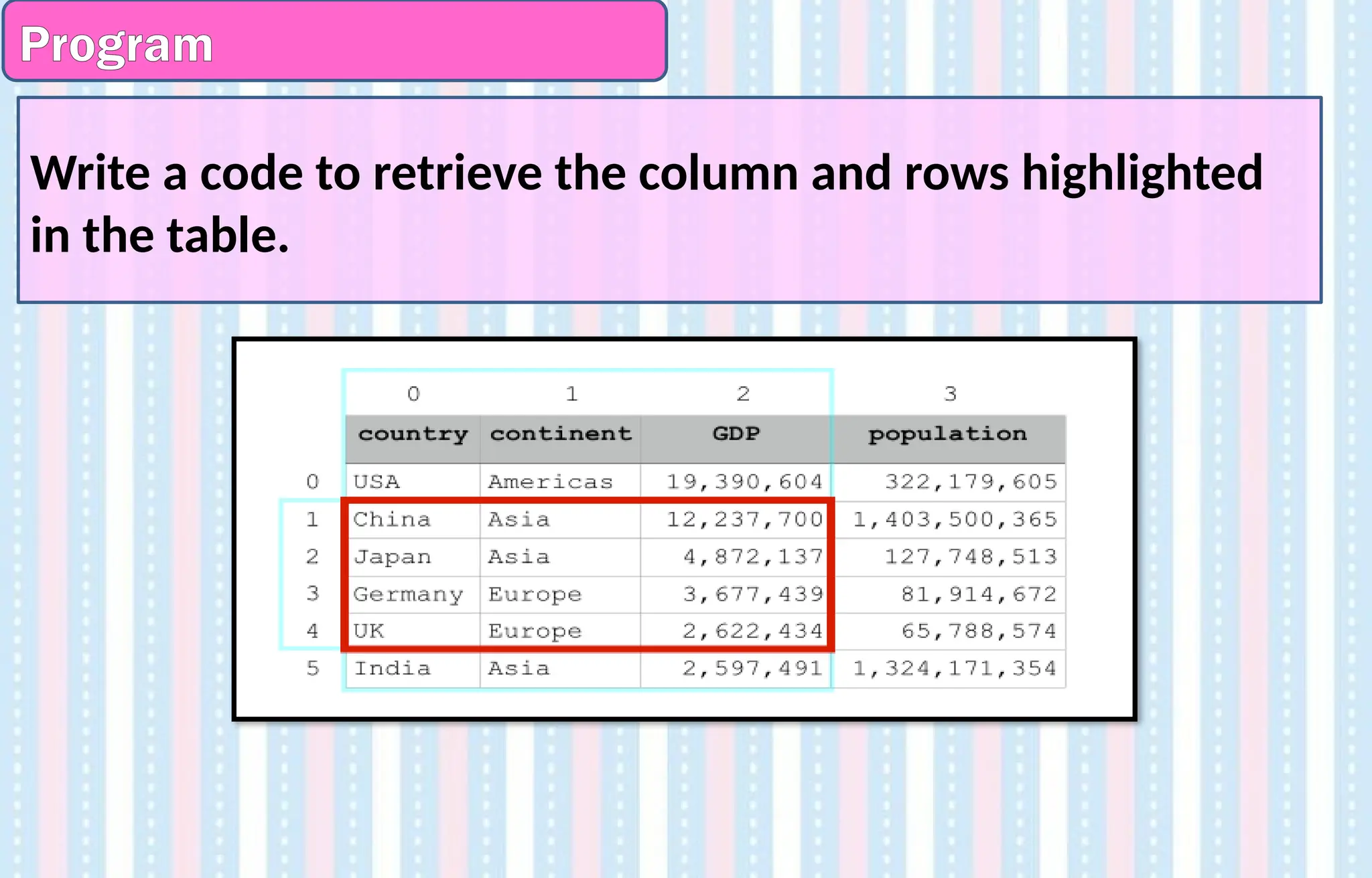
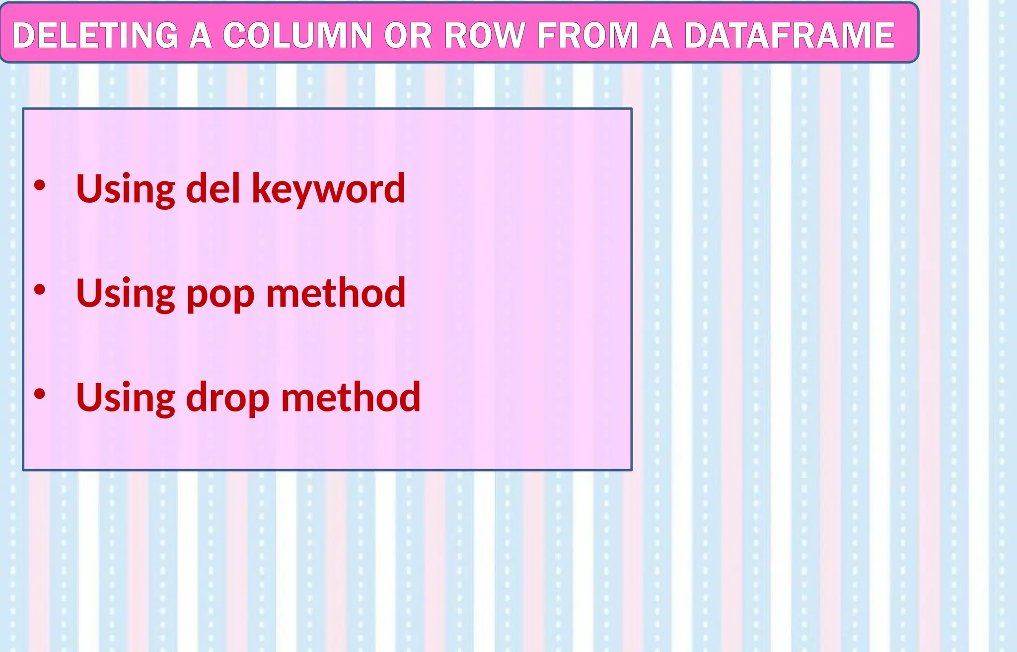
![DELETING A COLUMN FROM A DATAFRAME
• Using del keyword – [ONLY FOR COLUMN , 1 column at a time]
del df[‘<column name>’]
This will only delete the particular column , after which we have to display the
dataframe to see the changes.
>>> del df['Date']
>>> df
Event Cost
0 Music 10000
1 Poetry 5000
2 Theatre 15000
3 Comedy 2000](https://image.slidesharecdn.com/ln-250918173733-5ea4f2ca/75/Ln-1-Data-Handling-using-Pandas-I-1-pptx-143-2048.jpg)
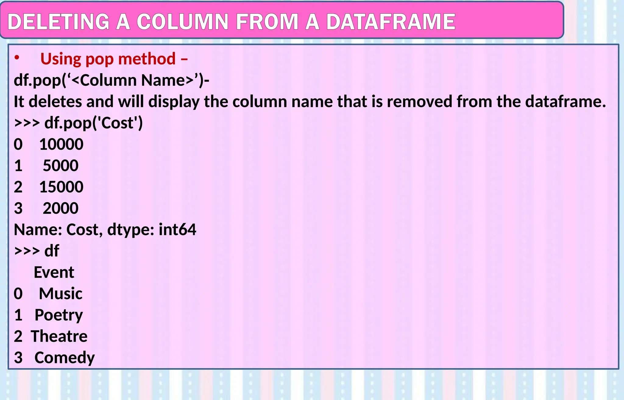
![DELETING A ROW OR COLUMN FROM A DATAFRAME
• Using drop method – drop (labels, axis=1)
It will return a new dataframe with the columns deleted. Axis=1 means column
and axis=0 means row. By default it is 0.
To remove any row,
>>> df.drop([0]) OR >>> df.drop([0],axis=0)
Date Event Cost
1 11/2/2011 Poetry 5000
2 12/2/2011 Theatre 15000
3 13/2/11 Comedy 2000
To remove any column,
>>> df.drop(['Date'],axis=1)
Event Cost
0 Music 10000
1 Poetry 5000
2 Theatre 15000
4 Comedy 2000
To remove a column permanently from your dataframe
you will need to provide one more parameter
inplace=True.](https://image.slidesharecdn.com/ln-250918173733-5ea4f2ca/75/Ln-1-Data-Handling-using-Pandas-I-1-pptx-145-2048.jpg)
![DELETING A ROW OR COLUMN FROM A DATAFRAME
• To delete multiple columns :
df.drop([‘Column1’, ‘Column2’], axis=1, inplace = True)
OR
df.drop(columns=[‘Column1’, ‘Column2’], axis=1, inplace = True)
To drop rows :
df.drop([‘row1’,’row2’], axis= 0, inplace = True)
OR
df.drop(index=[‘row1’,’row2’], axis=0, inplace = True)](https://image.slidesharecdn.com/ln-250918173733-5ea4f2ca/75/Ln-1-Data-Handling-using-Pandas-I-1-pptx-146-2048.jpg)
![DELETING A COLUMN - Practical Implementation
• Create a simple dataframe with a dictionary of lists, and column
names: name, year, orders, town.
• Remove the column orders from the dataframe using del df[]
• Remove the column ‘name’ using df.pop( )
• Remove the column town using df.drop ()](https://image.slidesharecdn.com/ln-250918173733-5ea4f2ca/75/Ln-1-Data-Handling-using-Pandas-I-1-pptx-147-2048.jpg)
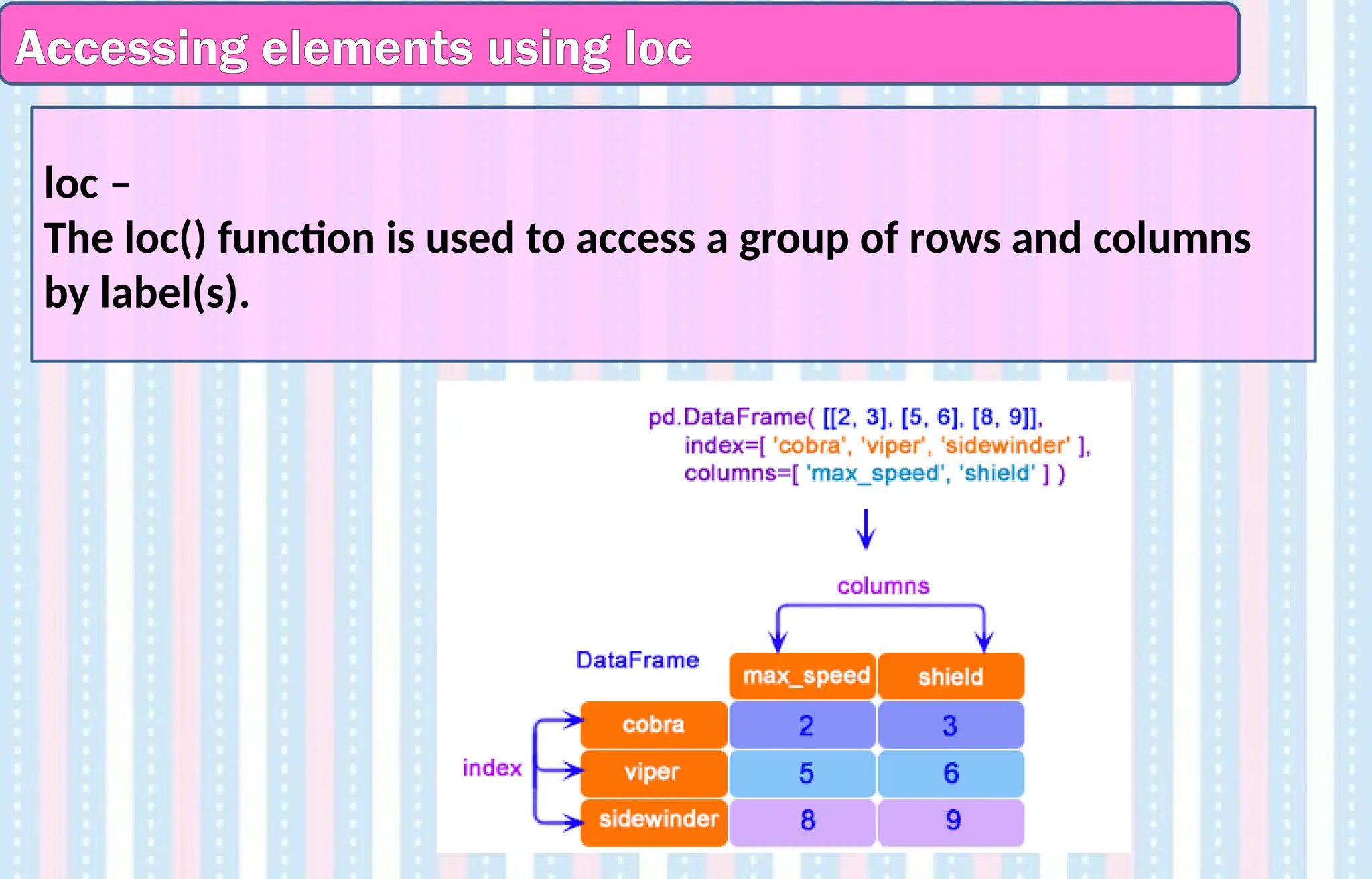
![Accessing elements using loc
>>>df = pd.DataFrame({"A":[12, 4, 5, None, 1],"B":[7, 2, 54, 3, None],
"C":[20, 16, 11, 3, 8], "D":[14, 3, None, 2, 6]})
>>> df.iloc[0,2]
20
>>> df.loc[0,'B']
7.0
>>> >>> df.iloc[0:2,0:2]
A B
0 12.0 7.0
1 4.0 2.0
>>> df.loc[0:2,"A":"C"]
A B C
0 12.0 7.0 20
1 4.0 2.0 16
2 5.0 54.0 11](https://image.slidesharecdn.com/ln-250918173733-5ea4f2ca/75/Ln-1-Data-Handling-using-Pandas-I-1-pptx-149-2048.jpg)
![Accessing elements using loc
>>> df.iloc[:,0:2]
A B
0 12.0 7.0
1 4.0 2.0
2 5.0 54.0
3 NaN 3.0
4 1.0 NaN
>>> df.loc[:,"A":"C"]
A B C
0 12.0 7.0 20
1 4.0 2.0 16
2 5.0 54.0 11
3 NaN 3.0 3
4 1.0 NaN 8
>>> df.iloc[[1,3],[2,1]]
C B
1 16 2.0
3 3 3.0
>>> df.loc[[1,3],
["A","C"]]
A C
1 4.0 16
3 NaN 3](https://image.slidesharecdn.com/ln-250918173733-5ea4f2ca/75/Ln-1-Data-Handling-using-Pandas-I-1-pptx-150-2048.jpg)
![Head and Tail in DataFrame
The method head() gives the first 5
rows and tail gives the last 5.
import pandas as pd
emp={'id':
[100,101,102,103,105,106,107],'na
me':
['Raj','Sini','Flora','Leena','Priya','De
nny','Kevin'],'Sal':
[12000,5000,2200,3200,23000,8700,
15000]}
df=pd.DataFrame(emp)
print(df)
print(df.head())
print(df.tail())
print(df.head(2))
print(df.tail(3))
id name Sal
0 100 Raj 12000
1 101 Sini 5000
2 102 Flora 2200
3 103 Leena 3200
4 105 Priya 23000
5 106 Denny 8700
6 107 Kevin 15000
id name Sal
0 100 Raj 12000
1 101 Sini 5000
2 102 Flora 2200
3 103 Leena 3200
4 105 Priya 23000
id name Sal
2 102 Flora 2200
3 103 Leena 3200
4 105 Priya 23000
5 106 Denny 8700
6 107 Kevin 15000
id name Sal
0 100 Raj 12000
7 101 Sini 5000
id name Sal
4 105 Priya 23000
5 106 Denny 8700
6 107 Kevin 15000](https://image.slidesharecdn.com/ln-250918173733-5ea4f2ca/75/Ln-1-Data-Handling-using-Pandas-I-1-pptx-151-2048.jpg)
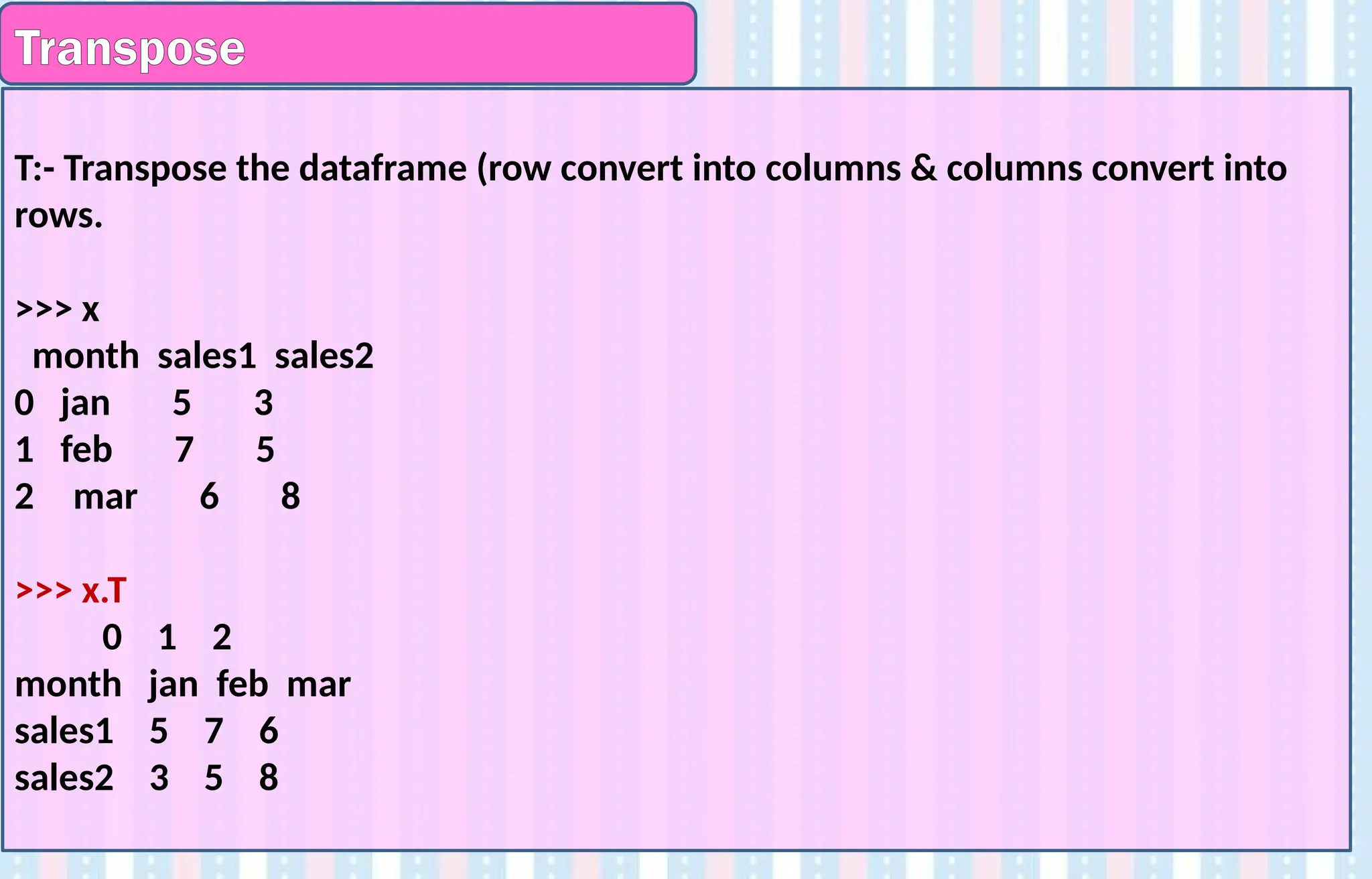
![reindex
Reindex will change the order of index .
>>> x=pd.DataFrame({'month':['jan','feb','mar'], 'sales1':[5,7,6],'sales2':[3,5,8]})
>>> x
month sales1 sales2
0 jan 5 3
1 feb 7 5
2 mar 6 8
>>> y=x.reindex([2,1,0])
>>> y
month sales1 sales2
2 mar 6 8
1 feb 7 5
0 jan 5 3](https://image.slidesharecdn.com/ln-250918173733-5ea4f2ca/75/Ln-1-Data-Handling-using-Pandas-I-1-pptx-153-2048.jpg)
![Binary operations
Pandas provides the methods add(), sub(), mul(), div() for carrying out binary
operations on dataframes.
Since all these operations involve 2 dataframes to act upon, they are called
Binary. (‘bi’ means ‘two’ and ‘ary’ means digits)
>>> S1=pd.DataFrame({'UT-1':[23,20,21,19,25],'UT-2':[20,23,12,16,23]})
>>> S2=pd.DataFrame({'UT-1':[13,21,22,10,21],'UT-2':[24,23,11,12,24]})
>>> S1.add(S2)
UT-1 UT-2
0 36 44
1 41 46
2 43 23
3 29 28
4 46 47](https://image.slidesharecdn.com/ln-250918173733-5ea4f2ca/75/Ln-1-Data-Handling-using-Pandas-I-1-pptx-154-2048.jpg)
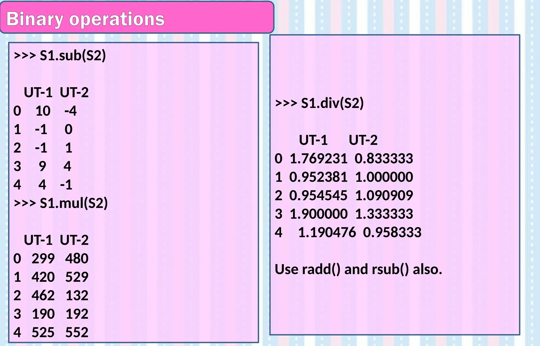
![1.Write the purpose of the following statement:
mtns_df.set_index('name', inplace=True)
2. Write the output of the statement:
a. mtns.loc[:, 'summited’]
b. mtns.loc['K2', :]
c. mtns.loc['K2', 'summited’]
d. mtns.loc[['K2', 'Lhotse'], :]
e. mtns.loc[:, 'height': 'summited’]
f. mtns.loc[mtns.loc[:, 'summited'] > 1954, :]
g. mtns.iloc[0, :]
h. mtns.iloc[:, 2]
i. mtns.iloc[0, 2]
j. mtns.iloc[[1, 3], :]
k. mtns.iloc[:, 0:2]](https://image.slidesharecdn.com/ln-250918173733-5ea4f2ca/75/Ln-1-Data-Handling-using-Pandas-I-1-pptx-156-2048.jpg)
![Accessing a DataFrame with a boolean index
• We can create Boolean indexes for dataFrames and searching can be done
based on True or False indexes.
• loc() is used.
• Pandas, DataFrame also support Boolean indexing.
• So we can direct search our data based on True or False indexing.
• We can use loc[ ] for this purpose.
• In order to access a dataframe with a boolean index, we have to create a
dataframe in which index of dataframe contains a boolean value that is
“True” or “False”.
import pandas as pd
dict= {'name':[“Mohak", “Freya", “Roshni"], 'degree': ["MBA", "BCA", "M.Tech"],
'score':[90, 40, 80]}
df= pd.DataFrame(dict, index = [True, False, True])
print(df.loc[True])](https://image.slidesharecdn.com/ln-250918173733-5ea4f2ca/75/Ln-1-Data-Handling-using-Pandas-I-1-pptx-157-2048.jpg)
![Accessing a DataFrame with a boolean index
import pandas as pd
data1={ 'rollno' : [101,102,103,104],
'name' : ['ram','mohan','sohan','rohan'] }
student1 = pd.DataFrame(data1,
index = [True, False, True, False],
columns=['rollno' , 'name']
)
print(student1)
Output rollno name
True 101 ram
False 102 mohan
True 103 sohan
False 104 rohan
print(student1.loc[True] )
Output rollno name
True 101 ram
True 103 sohan
-----------------------
print(student1.loc[False] )
Output rollno name
False 102 mohan
False 104 rohan](https://image.slidesharecdn.com/ln-250918173733-5ea4f2ca/75/Ln-1-Data-Handling-using-Pandas-I-1-pptx-158-2048.jpg)
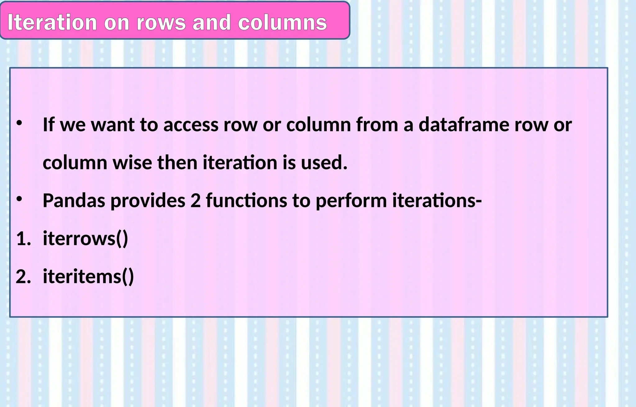
![iterrows
• It is used to access the data row wise.
import pandas as pd
ab= [{'Name':'Arya','Age':20},{'Name':'Shane','Age':19}]
df=pd.DataFrame(ab)
for(i,j) in df.iterrows():
print(j)
Name Arya
Age 20
Name: 0, dtype: object
Name Shane
Age 19
Name: 1, dtype: object](https://image.slidesharecdn.com/ln-250918173733-5ea4f2ca/75/Ln-1-Data-Handling-using-Pandas-I-1-pptx-160-2048.jpg)
![iteritems
• It is used to access the data column wise.
import pandas as pd
ab= [{'Name':'Arya','Age':20},{'Name':'Shane','Age':19}]
df=pd.DataFrame(ab)
for(i,j) in df.iteritems():
print(j)
0 Arya
1 Shane
Name: Name, dtype: object
0 20
1 19
Name: Age, dtype: int64](https://image.slidesharecdn.com/ln-250918173733-5ea4f2ca/75/Ln-1-Data-Handling-using-Pandas-I-1-pptx-161-2048.jpg)
![Basic functions
>>> x=pd.DataFrame({ 'month':
['jan','feb', 'mar'], 'sales1':[5,7,6],
'sales2':[3,5,8]})
>>> x
month sales1 sales2
0 jan 5 3
1 feb 7 5
2 mar 6 8
>>> x.count()
month 3
sales1 3
sales2 3
dtype: int64
>>> x.max()
month mar
sales1 7
sales2 8
dtype: object
>>> x.min()
month feb
sales1 5
sales2 3
dtype: object
>>> x.sum()
month janfebmar
sales1 18
sales2 16
dtype: object](https://image.slidesharecdn.com/ln-250918173733-5ea4f2ca/75/Ln-1-Data-Handling-using-Pandas-I-1-pptx-162-2048.jpg)

![To fill NaN with desire data in particular column data
import pandas as pd
import numpy as np
data1={'rollno' : [101, 102, 103, 104],
'name' : ['ram','mohan',’sohan’,
np.NaN]}
student1 = pd.DataFrame(data1,
columns=['rollno' , 'name'] )
print(student1)
O/p-
Rollno name
0 101 ram
1 102 mohan
2 103 sohan
3 104 np.NaN
>>> student1 ['name'] . fillna( 'rohit',
inplace = True)
>>> student1
rollno name
0 101 ram
1 102 mohan
2 103 sohan
3 104 rohit
student1. fillna( 999, inplace = True)
print(df)
rollno name
0 101 ram
1 102 mohan
2 103 sohan
3 104 999](https://image.slidesharecdn.com/ln-250918173733-5ea4f2ca/75/Ln-1-Data-Handling-using-Pandas-I-1-pptx-164-2048.jpg)
![Adding a new row using - append() method
import pandas as pd
data1={'rollno' : [101,102],
'name' : ['ram','mohan']}
student1 = pd.DataFrame(data1,
columns=['rollno' , 'name'] )
print(student1)
rollno name
0 101 ram
1 102 mohan
#to add a new row in existing a
DataFrame
Student1= student1.append({ 'rollno' :
103, 'name': 'sohan' } ,ignore_index
=True)
print(student1)
rollno name
0 101 ram
1 102 mohan
2 103 sohan](https://image.slidesharecdn.com/ln-250918173733-5ea4f2ca/75/Ln-1-Data-Handling-using-Pandas-I-1-pptx-165-2048.jpg)
![Handling missing values (NaN) – dropping Using dropna() method
>>> import pandas as pd
>>>import numpy as np;
>>>data1={'rollno' : [101, 102,
103, 104],'name' :
['ram','mohan','sohan', np.NaN]}
student1 = pd.DataFrame(data1,
columns=['rollno' , 'name'] )
print(student1)
rollno name
0 101 ram
1 102 mohan
2 103 sohan
3 104 NaN
#to drop, all rows of NaN by default
student1 . dropna( inplace = True)
student1
rollno name
0 101 ram
1 102 mohan
2 103 sohan
#to drop, NaN of all column using axis =1
student1 . dropna(axis=1, inplace =
True)
print(student1)](https://image.slidesharecdn.com/ln-250918173733-5ea4f2ca/75/Ln-1-Data-Handling-using-Pandas-I-1-pptx-166-2048.jpg)
![To check if zero exists
data1 = {'rollno' : [101, 102, 103, 104],'name' :
['ram', 'mohan', 'sohan', 'rohan']}
student = pd.DataFrame(data1,
columns=['rollno','name'])
print(student)
rollno name
0 101 ram
1 102 mohan
2 103 sohan
3 104 rohan
>>> student.all()
rollno True
name True
dtype: bool
>>> student.all(axis=1)
0 True
1 True
2 True
3 True
dtype: bool
>>> data1 = {'rollno' : [0, 102, 103, 104],'name' :
['ram', 0, 'sohan', 'rohan']}
student = pd.DataFrame(data1,
columns=['rollno','name'])
print(student)
rollno name
0 0 ram
1 102 0
2 103 sohan
3 104 rohan
>>> student.all()
rollno False
name False
dtype: bool
>>> student.all(axis=1)
0 False
1 False
2 True
3 True
dtype: bool
all() returns whether all
elements are True over
the requested axis.](https://image.slidesharecdn.com/ln-250918173733-5ea4f2ca/75/Ln-1-Data-Handling-using-Pandas-I-1-pptx-167-2048.jpg)

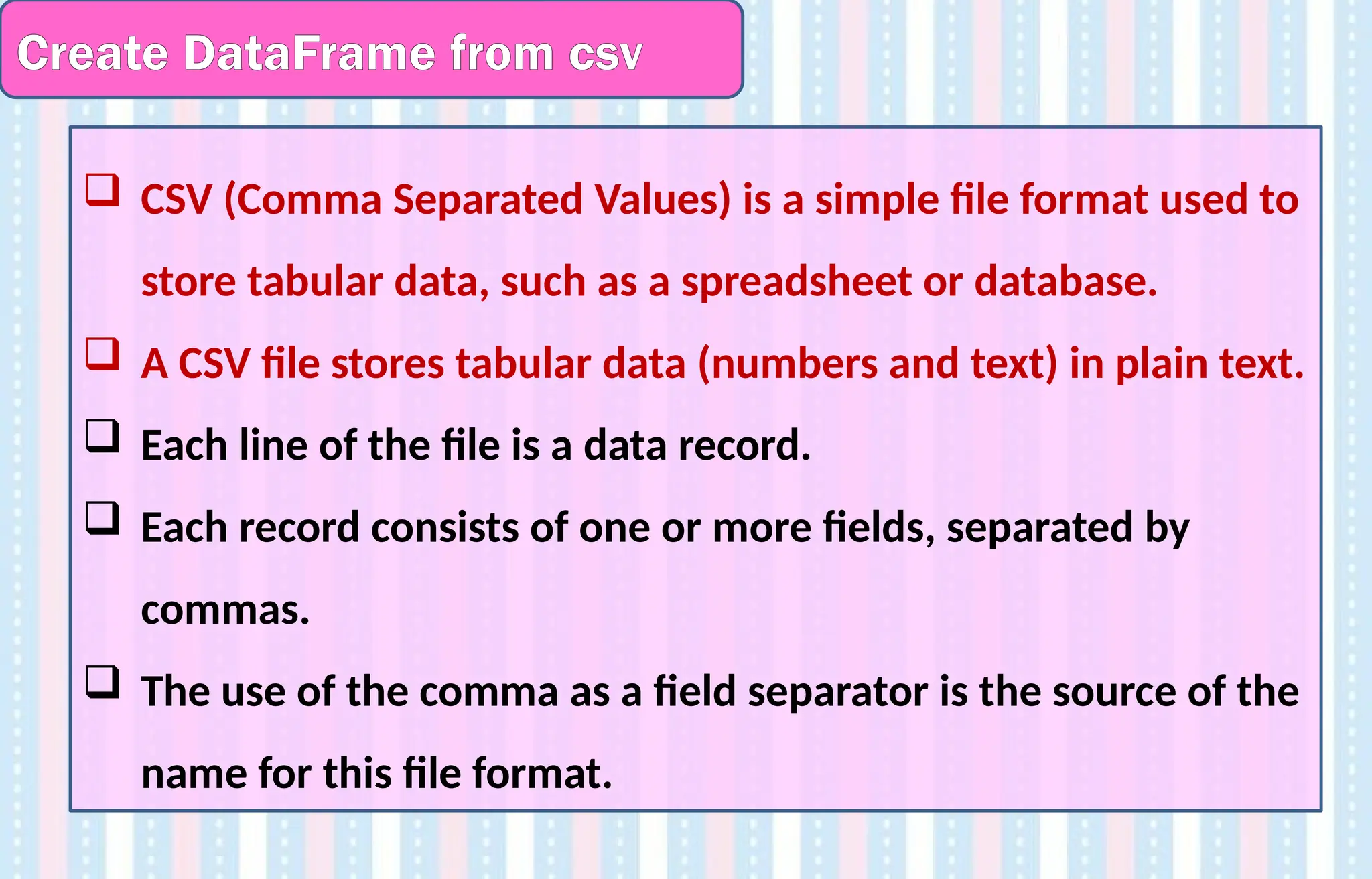


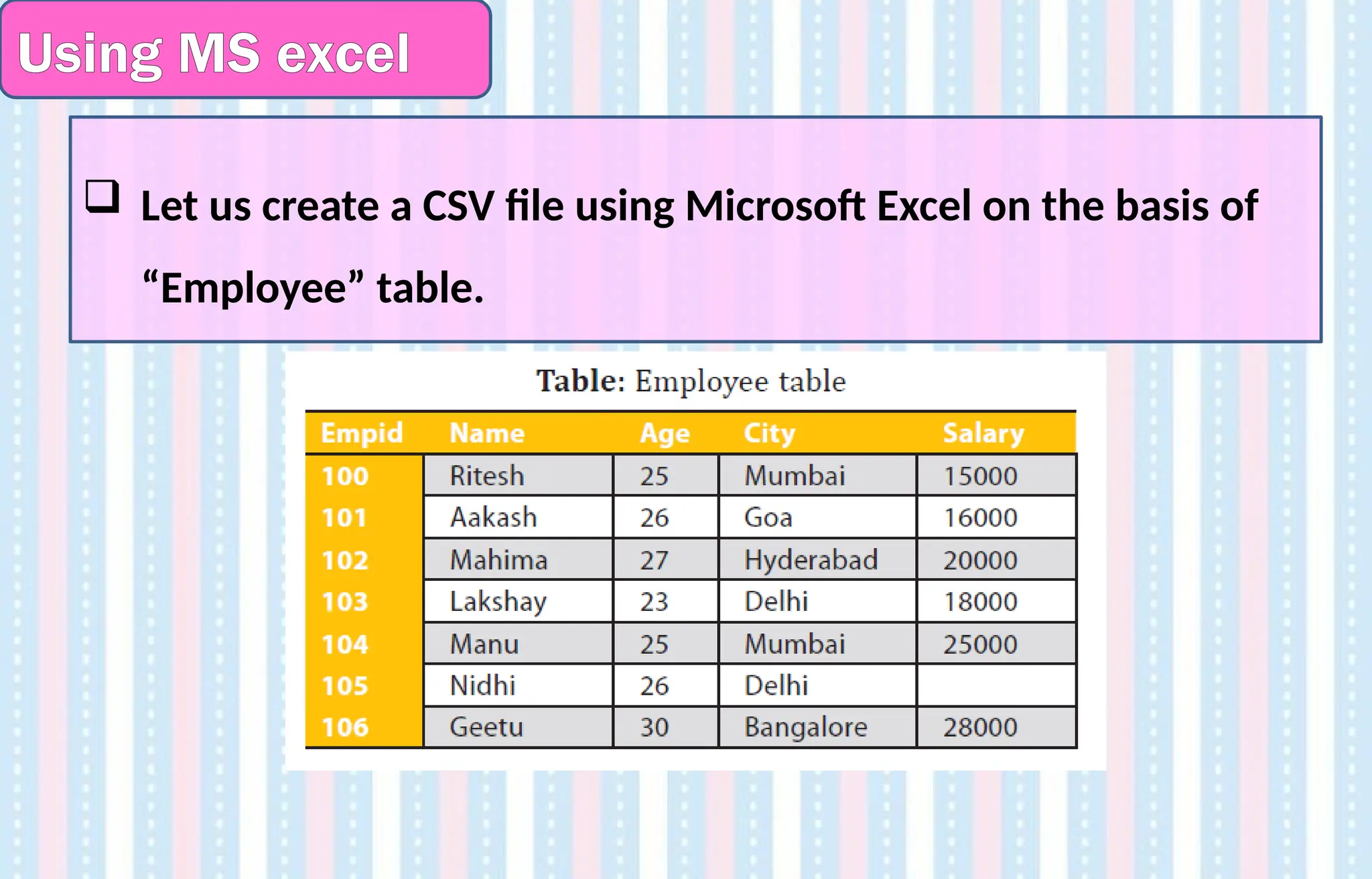
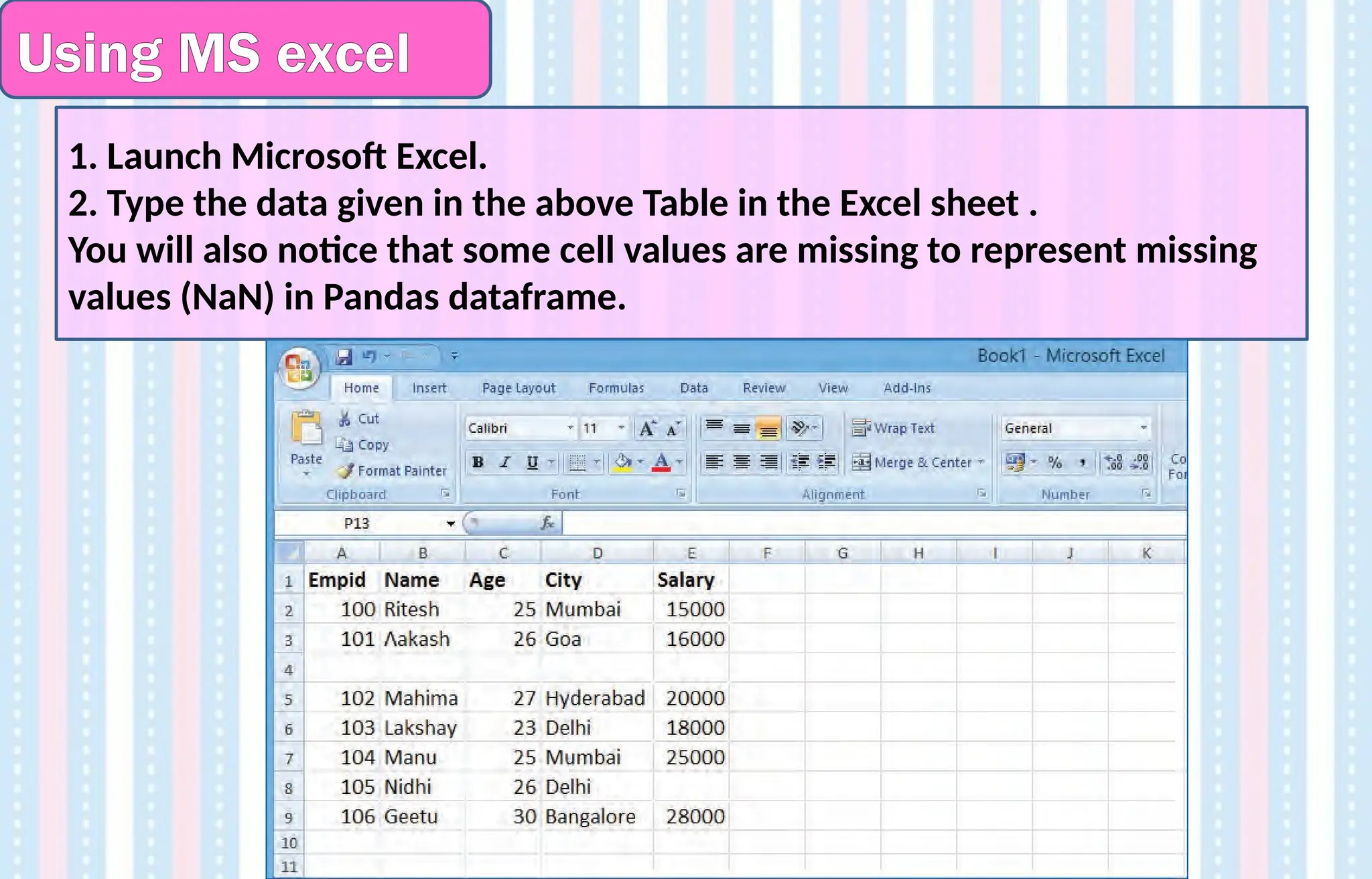


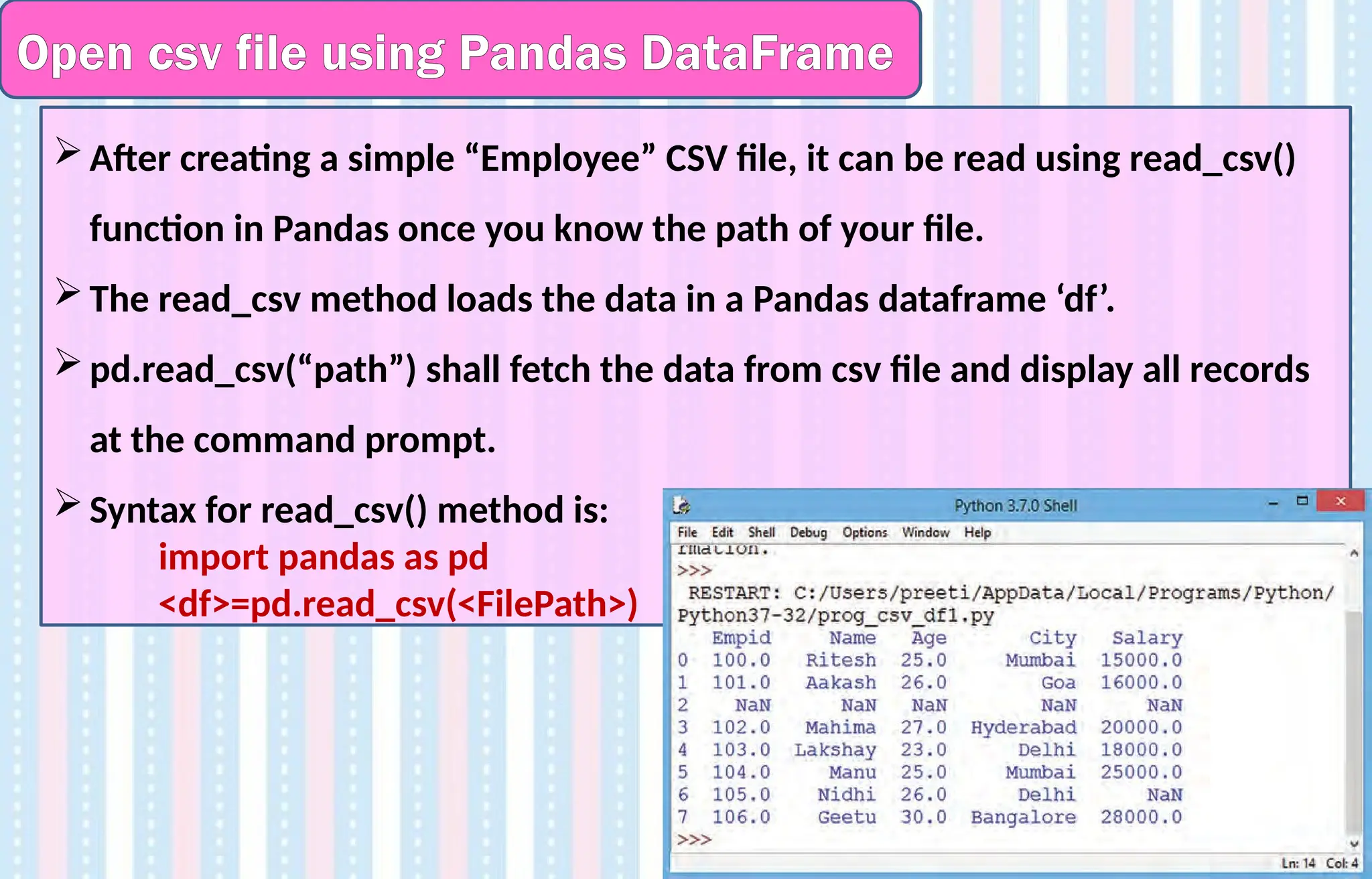
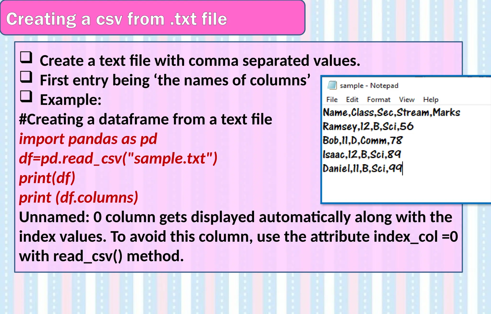
![More commands
• To display the shape (number of rows and columns) of the CSV file
df.shape
>>> df.shape
(7, 5)
Reading CSV file with specific/selected columns-
• This can be done by using “usecols” attribute along with read_csv().
>>> df=pd.read_csv("Employee.csv",usecols=['Name','Age'])
Reading CSV file with specific/selected rows-
• Use “nrows” attribute used with read_csv(). nrows means number of
rows.
>>> df=pd.read_csv("Employee.csv",nrows=5)
• Here 5 rows are displayed. It will display NaN values also, if present.](https://image.slidesharecdn.com/ln-250918173733-5ea4f2ca/75/Ln-1-Data-Handling-using-Pandas-I-1-pptx-179-2048.jpg)
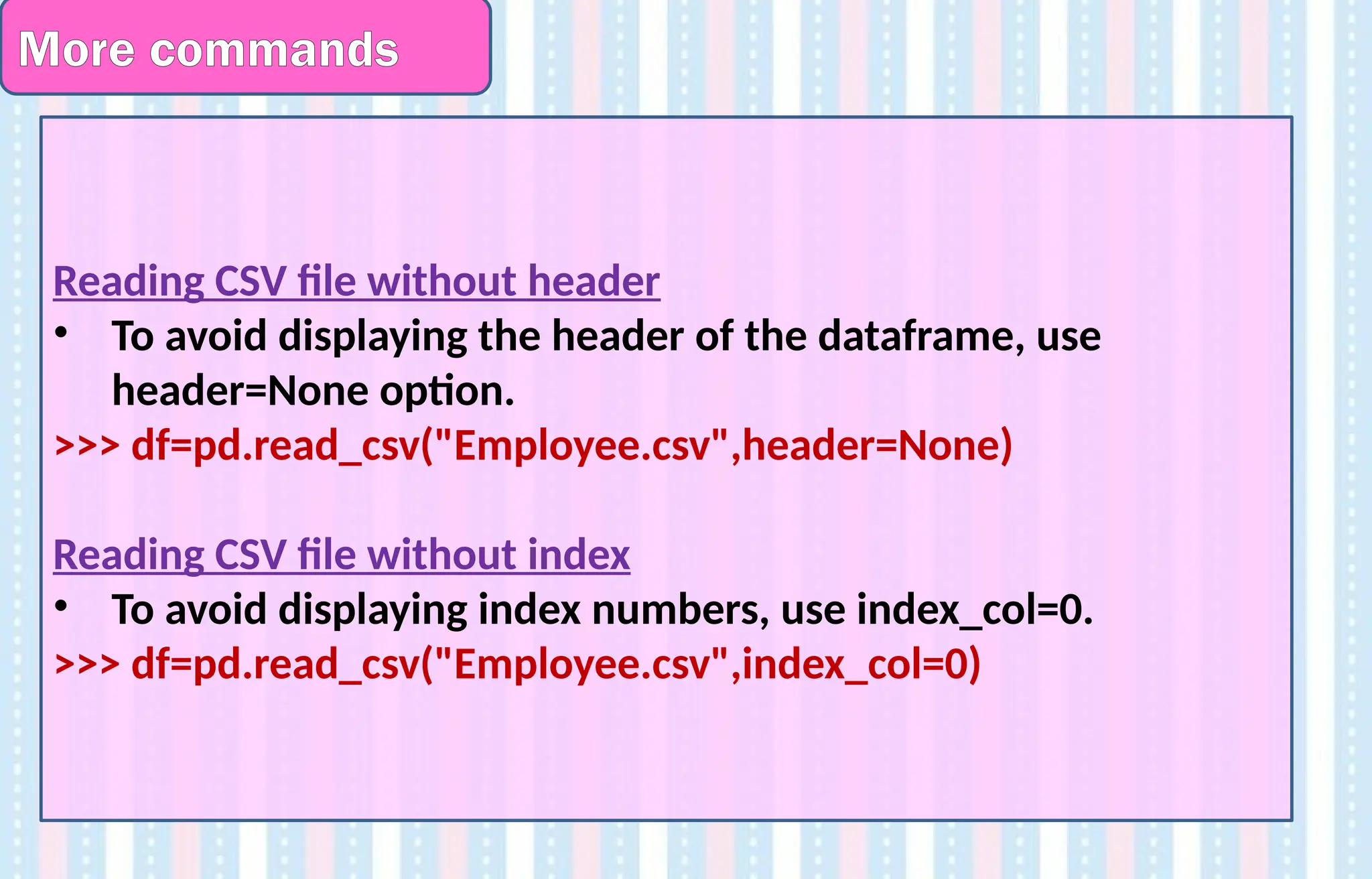
![UPDATING/MODIFYING CONTENTS IN A CSV FILE
Reading CSV file with new column names
• Use skiprow option to skip the header if it exists. Specify the new
names with names option.
df=pd.read_csv("Employee.csv",skiprows=1,names=['a','b','c','d','e'])
Replace any contents of the dataframe with NaN values-
• Done by using na_values option along with read_csv method
>>> df=pd.read_csv("Employee.csv",na_values=[26])
Here wherever the value 26 is seen, it gets updated to NaN.](https://image.slidesharecdn.com/ln-250918173733-5ea4f2ca/75/Ln-1-Data-Handling-using-Pandas-I-1-pptx-181-2048.jpg)
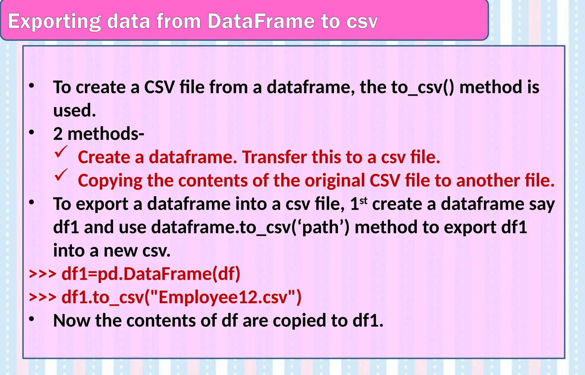
![Example
import pandas as pd
cars = {'Brand': ['Honda Civic','ToyotaCorolla',
'FordFocus','AudiA4'],'Price': [22000,25000,27000,35000]}
df= pd.DataFrame(cars, columns= ['Brand', 'Price'])
df.to_csv('export_dataframe.csv', index = False, header=True)
#Open the notepad with export_dataframe file.
pd.read_csv('export_dataframe.csv')](https://image.slidesharecdn.com/ln-250918173733-5ea4f2ca/75/Ln-1-Data-Handling-using-Pandas-I-1-pptx-183-2048.jpg)