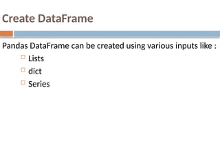
Pandas is a powerful Python library designed for data manipulation and analysis, providing expressive data structures such as Series and DataFrames. It facilitates the processing of data through functionalities like loading, preparing, manipulating, modeling, and analyzing data across various fields. Pandas also offers efficient tools for handling missing data, reshaping datasets, and performing data preprocessing tasks essential for machine learning applications.


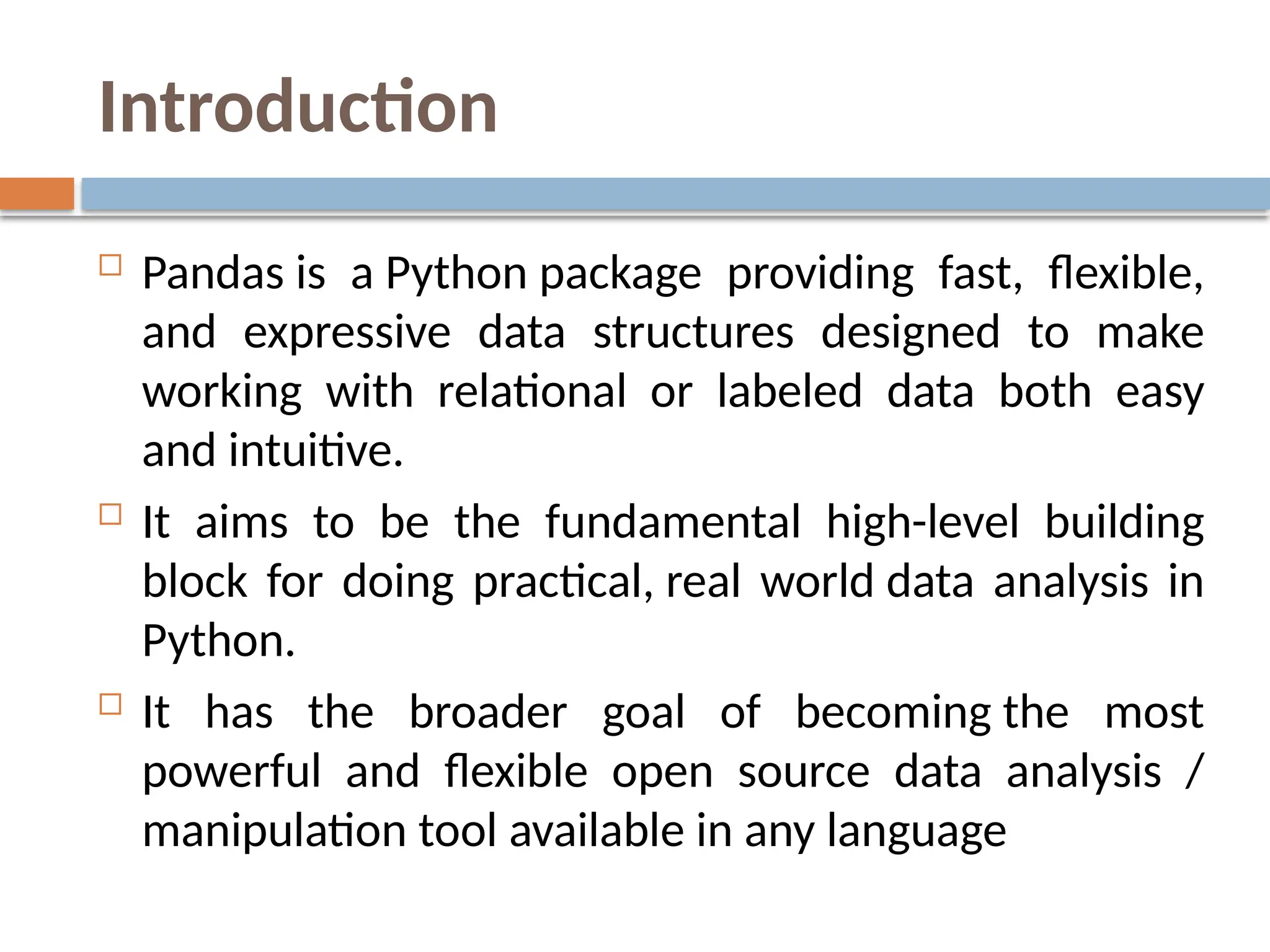
![Create a Series by array
If data is an ndarray, then index passed must be of
the same length. If no index is passed, then by
default index will be range(n) where n is array length,
i.e., [0,1,2,3…. range(len(array))-1].
Ex: series_1.py
import pandas as pd
import numpy as np
data = np.array(['a','b','c','d'])
s = pd.Series(data)
print (s)](https://image.slidesharecdn.com/python-pandas-240805090816-2e57e9f1/85/python-pandas-For-Data-Analysis-Manipulate-pptx-12-320.jpg)


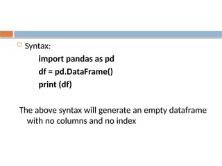


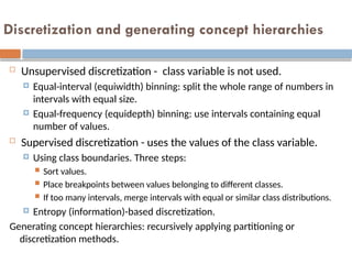
![Data transformation
Normalization:
Scaling attribute values to fall within a specified range.
Example: to transform V in [min, max] to V' in [0,1],
apply V'=(V-Min)/(Max-Min)
Scaling by using mean and standard deviation (useful when min
and max are unknown or when there are
outliers): V'=(V-Mean)/StDev
Aggregation: moving up in the concept hierarchy on numeric
attributes.
Generalization: moving up in the concept hierarchy on nominal
attributes.
Attribute construction: replacing or adding new attributes
inferred by existing attributes.](https://image.slidesharecdn.com/python-pandas-240805090816-2e57e9f1/85/python-pandas-For-Data-Analysis-Manipulate-pptx-28-320.jpg)
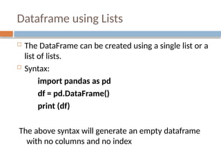
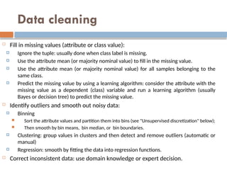
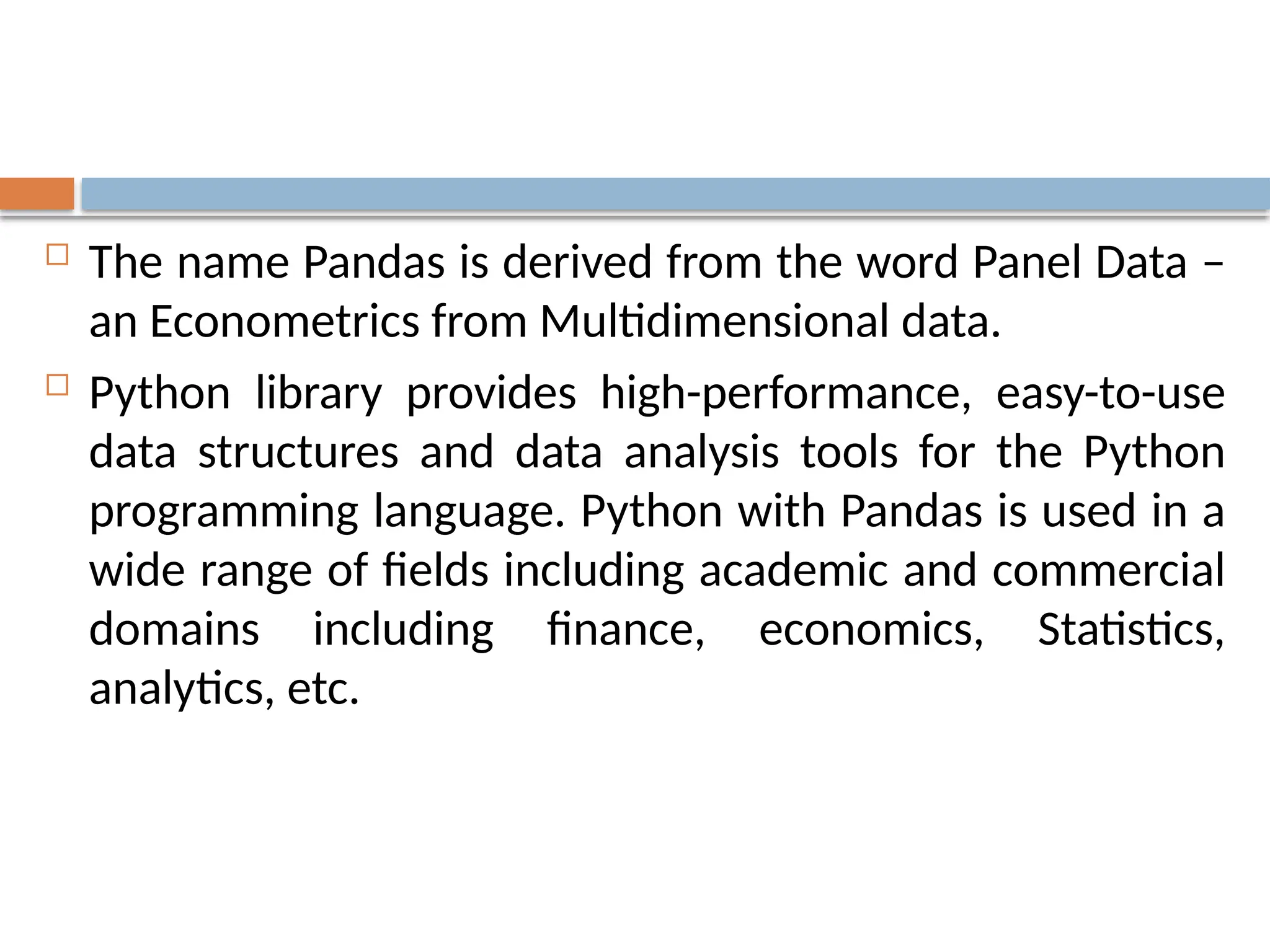
![Missing Values in the array set or the Dataset
Identifying the no. of missing values in a dataset.
Function: - data.isna() or data.isnull()
The above function returns true if the dataframe or
dataset is having null values.
We can also count the number of null values in a column.
Function:- data.isnull().sum() or data.isna().sum()
data.isnull().sum(axis=0) [column level] /
data.isnull().sum(axis=1) [row level]](https://image.slidesharecdn.com/python-pandas-240805090816-2e57e9f1/85/python-pandas-For-Data-Analysis-Manipulate-pptx-31-320.jpg)

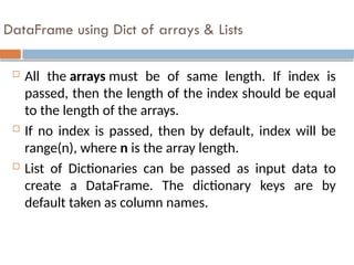
![Create a Series by array
If data is an ndarray, then index passed must be of
the same length. If no index is passed, then by
default index will be range(n) where n is array length,
i.e., [0,1,2,3…. range(len(array))-1].
Ex: series_1.py
import pandas as pd
import numpy as np
data = np.array(['a','b','c','d'])
s = pd.Series(data)
print (s)](https://image.slidesharecdn.com/python-pandas-240805090816-2e57e9f1/75/python-pandas-For-Data-Analysis-Manipulate-pptx-12-2048.jpg)


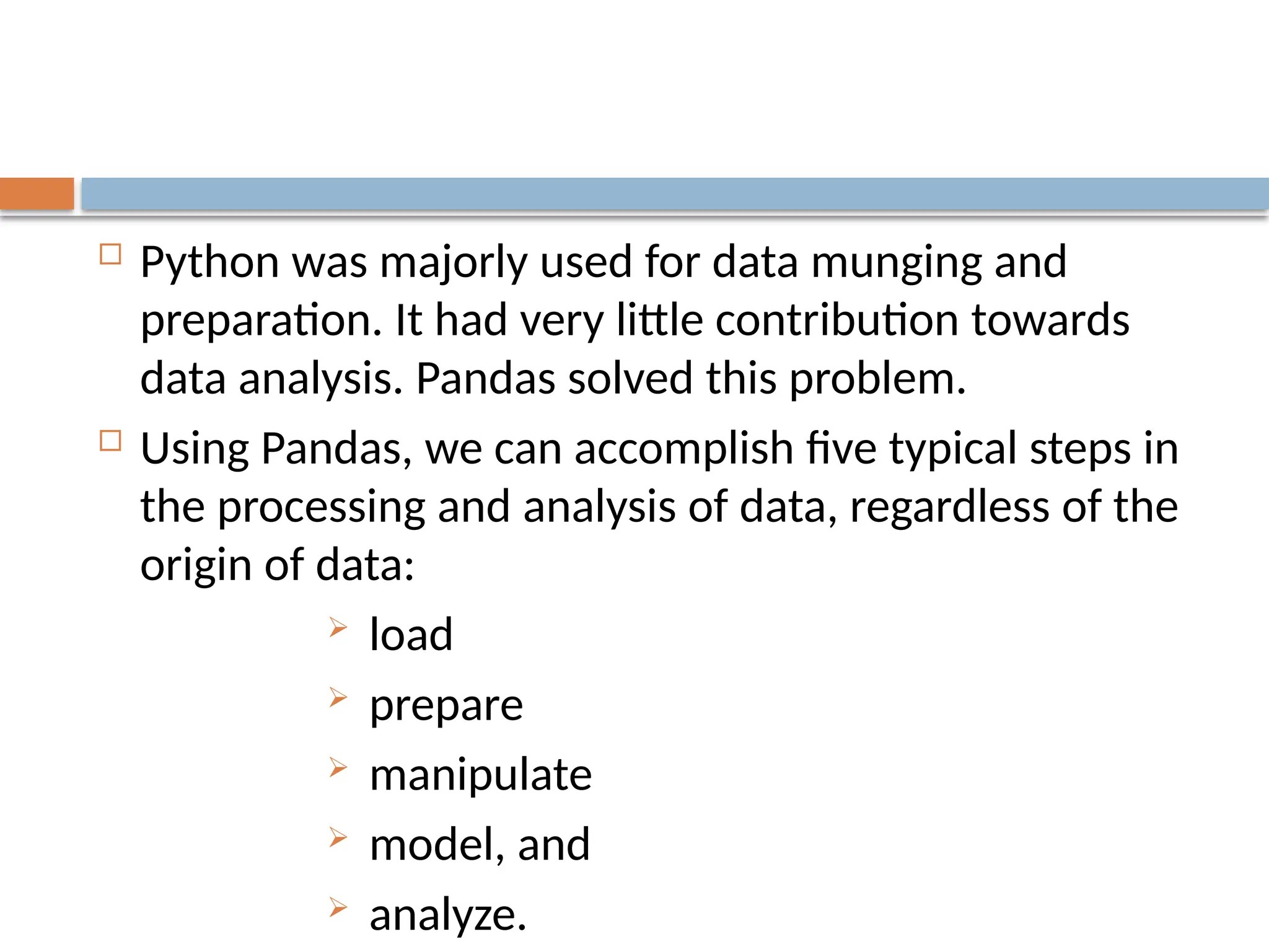
![Data transformation
Normalization:
Scaling attribute values to fall within a specified range.
Example: to transform V in [min, max] to V' in [0,1],
apply V'=(V-Min)/(Max-Min)
Scaling by using mean and standard deviation (useful when min
and max are unknown or when there are
outliers): V'=(V-Mean)/StDev
Aggregation: moving up in the concept hierarchy on numeric
attributes.
Generalization: moving up in the concept hierarchy on nominal
attributes.
Attribute construction: replacing or adding new attributes
inferred by existing attributes.](https://image.slidesharecdn.com/python-pandas-240805090816-2e57e9f1/75/python-pandas-For-Data-Analysis-Manipulate-pptx-28-2048.jpg)

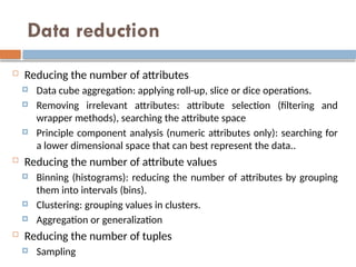
![Missing Values in the array set or the Dataset
Identifying the no. of missing values in a dataset.
Function: - data.isna() or data.isnull()
The above function returns true if the dataframe or
dataset is having null values.
We can also count the number of null values in a column.
Function:- data.isnull().sum() or data.isna().sum()
data.isnull().sum(axis=0) [column level] /
data.isnull().sum(axis=1) [row level]](https://image.slidesharecdn.com/python-pandas-240805090816-2e57e9f1/75/python-pandas-For-Data-Analysis-Manipulate-pptx-31-2048.jpg)


