Downloaded 192 times


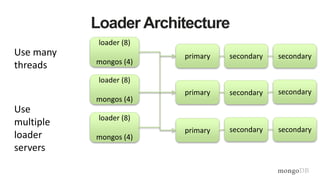
![Document Data Model
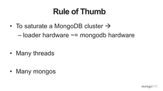
Relational MongoDB
{
first_name: ‘Paul’,
surname: ‘Miller’,
city: ‘London’,
location: [45.123,47.232],
cars: [
{ model: ‘Bentley’,
year: 1973,
value: 100000, … },
{ model: ‘Rolls Royce’,
year: 1965,
value: 330000, … }
]
}](https://image.slidesharecdn.com/mdbbestpracticesv11-151202171511-lva1-app68921-170405174543/85/MongoDB-Best-Practices-10-320.jpg)
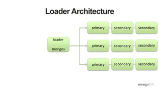
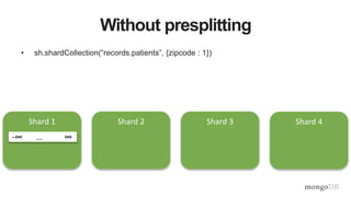
![Documents are Rich Data Structures
{
first_name: ‘Paul’,
surname: ‘Miller’,
cell: 447557505611,
city: ‘London’,
location: [45.123,47.232],
Profession: [‘banking’, ‘finance’, ‘trader’],
cars: [
{ model: ‘Bentley’,
year: 1973,
value: 100000, … },
{ model: ‘Rolls Royce’,
year: 1965,
value: 330000, … }
Fields can contain an array of
sub-documents
Fields
Typed fields
Fields can
contain arrays](https://image.slidesharecdn.com/mdbbestpracticesv11-151202171511-lva1-app68921-170405174543/85/MongoDB-Best-Practices-11-320.jpg)
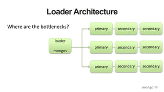
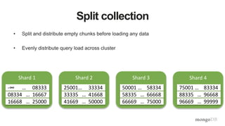
![Do More With Your Data
{
first_name: ‘Paul’,
surname: ‘Miller’,
city: ‘London’,
location: [45.123,47.232],
cars: [
{ model: ‘Bentley’,
year: 1973,
value: 100000, … },
{ model: ‘Rolls Royce’,
year: 1965,
value: 330000, … }
}
}
Rich Queries
Find everybody in London
with a car built between
1970 and 1980
Geospatial
Find all of the car owners
within 5km of Trafalgar Sq.
Text Search
Find all the cars described
as having leather seats
Aggregation
Calculate the average value
of Paul’s car collection
Map Reduce
What is the ownership
pattern of colors by
geography over time?
(is purple trending up in
China?)](https://image.slidesharecdn.com/mdbbestpracticesv11-151202171511-lva1-app68921-170405174543/85/MongoDB-Best-Practices-12-320.jpg)


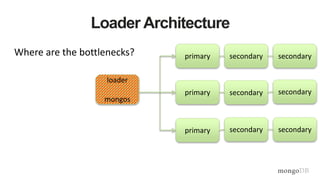
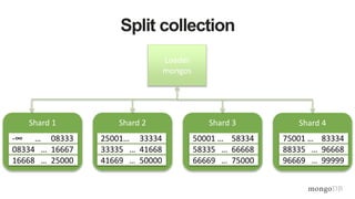
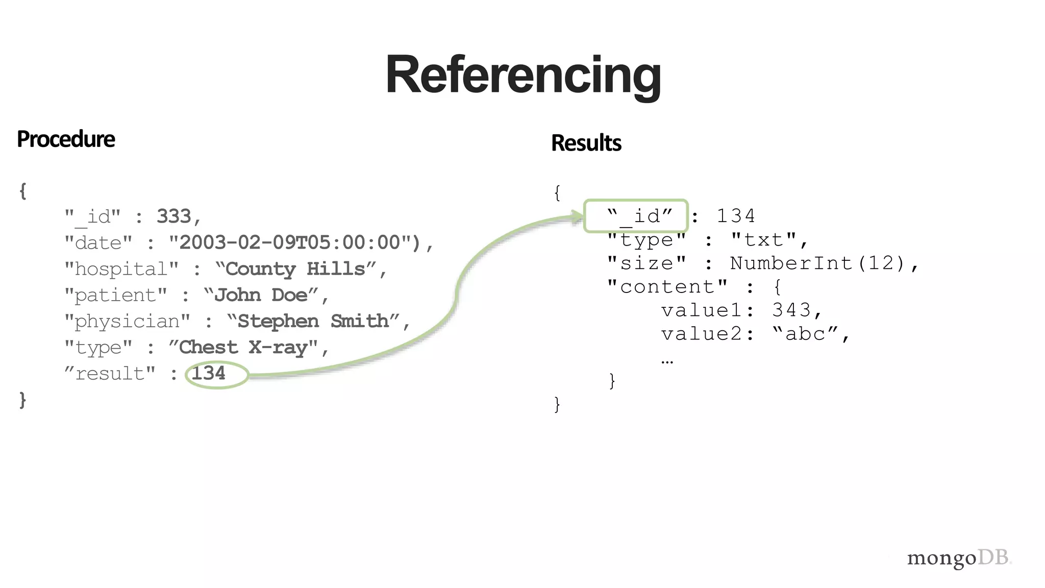
![{
_id: 2,
first: “Joe”,
last: “Patient”,
addr: { …},
procedures: [
{
id: 12345,
date: 2015-02-15,
type: “Cat scan”,
…},
{
id: 12346,
date: 2015-02-15,
type: “blood test”,
…}]
}
Patients
Embed
One-to-Many & Many-to-Many Relationships
{
_id: 2,
first: “Joe”,
last: “Patient”,
addr: { …},
procedures: [12345, 12346]}
{
_id: 12345,
date: 2015-02-15,
type: “Cat scan”,
…}
{
_id: 12346,
date: 2015-02-15,
type: “blood test”,
…}
Patients
Reference
Procedures](https://image.slidesharecdn.com/mdbbestpracticesv11-151202171511-lva1-app68921-170405174543/85/MongoDB-Best-Practices-45-320.jpg)


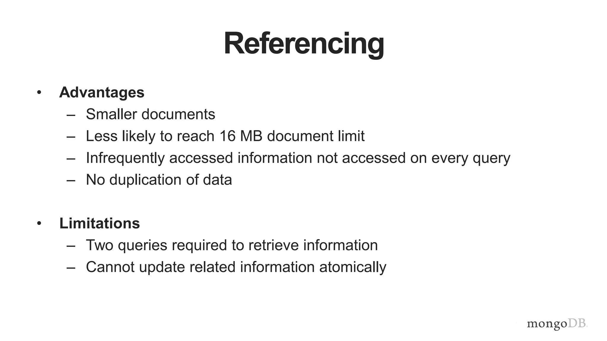
![Data From Vital Signs Monitoring Device
{
deviceId: 123456,
spO2: 88,
pulse: 74,
bp: [128, 80],
ts: ISODate("2013-10-16T22:07:00.000-0500")
}
• One document per minute per device
• Relational approach](https://image.slidesharecdn.com/mdbbestpracticesv11-151202171511-lva1-app68921-170405174543/85/MongoDB-Best-Practices-49-320.jpg)
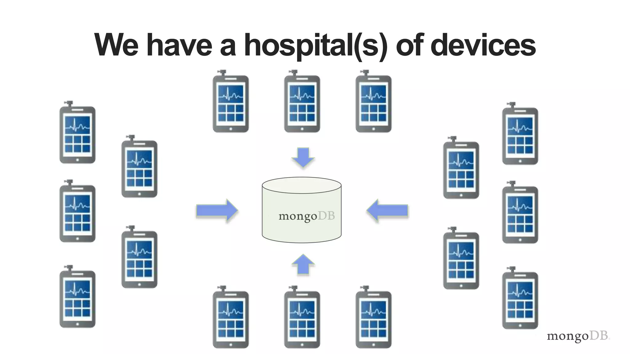
![Document Per Hour (By minute)
{
deviceId: 123456,
spO2: { 0: 88, 1: 90, …, 59: 92},
pulse: { 0: 74, 1: 76, …, 59: 72},
bp: { 0: [122, 80], 1: [126, 84], …, 59: [124, 78]},
ts: ISODate("2013-10-16T22:00:00.000-0500")
}
• Store per-minute data at the hourly level
• Update-driven workload
• 1 document per device per hour](https://image.slidesharecdn.com/mdbbestpracticesv11-151202171511-lva1-app68921-170405174543/85/MongoDB-Best-Practices-50-320.jpg)


![Document Data Model
Relational MongoDB
{
first_name: ‘Paul’,
surname: ‘Miller’,
city: ‘London’,
location: [45.123,47.232],
cars: [
{ model: ‘Bentley’,
year: 1973,
value: 100000, … },
{ model: ‘Rolls Royce’,
year: 1965,
value: 330000, … }
]
}](https://image.slidesharecdn.com/mdbbestpracticesv11-151202171511-lva1-app68921-170405174543/75/MongoDB-Best-Practices-10-2048.jpg)
![Documents are Rich Data Structures
{
first_name: ‘Paul’,
surname: ‘Miller’,
cell: 447557505611,
city: ‘London’,
location: [45.123,47.232],
Profession: [‘banking’, ‘finance’, ‘trader’],
cars: [
{ model: ‘Bentley’,
year: 1973,
value: 100000, … },
{ model: ‘Rolls Royce’,
year: 1965,
value: 330000, … }
Fields can contain an array of
sub-documents
Fields
Typed fields
Fields can
contain arrays](https://image.slidesharecdn.com/mdbbestpracticesv11-151202171511-lva1-app68921-170405174543/75/MongoDB-Best-Practices-11-2048.jpg)
![Do More With Your Data
{
first_name: ‘Paul’,
surname: ‘Miller’,
city: ‘London’,
location: [45.123,47.232],
cars: [
{ model: ‘Bentley’,
year: 1973,
value: 100000, … },
{ model: ‘Rolls Royce’,
year: 1965,
value: 330000, … }
}
}
Rich Queries
Find everybody in London
with a car built between
1970 and 1980
Geospatial
Find all of the car owners
within 5km of Trafalgar Sq.
Text Search
Find all the cars described
as having leather seats
Aggregation
Calculate the average value
of Paul’s car collection
Map Reduce
What is the ownership
pattern of colors by
geography over time?
(is purple trending up in
China?)](https://image.slidesharecdn.com/mdbbestpracticesv11-151202171511-lva1-app68921-170405174543/75/MongoDB-Best-Practices-12-2048.jpg)


![{
_id: 2,
first: “Joe”,
last: “Patient”,
addr: { …},
procedures: [
{
id: 12345,
date: 2015-02-15,
type: “Cat scan”,
…},
{
id: 12346,
date: 2015-02-15,
type: “blood test”,
…}]
}
Patients
Embed
One-to-Many & Many-to-Many Relationships
{
_id: 2,
first: “Joe”,
last: “Patient”,
addr: { …},
procedures: [12345, 12346]}
{
_id: 12345,
date: 2015-02-15,
type: “Cat scan”,
…}
{
_id: 12346,
date: 2015-02-15,
type: “blood test”,
…}
Patients
Reference
Procedures](https://image.slidesharecdn.com/mdbbestpracticesv11-151202171511-lva1-app68921-170405174543/75/MongoDB-Best-Practices-45-2048.jpg)


![Data From Vital Signs Monitoring Device
{
deviceId: 123456,
spO2: 88,
pulse: 74,
bp: [128, 80],
ts: ISODate("2013-10-16T22:07:00.000-0500")
}
• One document per minute per device
• Relational approach](https://image.slidesharecdn.com/mdbbestpracticesv11-151202171511-lva1-app68921-170405174543/75/MongoDB-Best-Practices-49-2048.jpg)
![Document Per Hour (By minute)
{
deviceId: 123456,
spO2: { 0: 88, 1: 90, …, 59: 92},
pulse: { 0: 74, 1: 76, …, 59: 72},
bp: { 0: [122, 80], 1: [126, 84], …, 59: [124, 78]},
ts: ISODate("2013-10-16T22:00:00.000-0500")
}
• Store per-minute data at the hourly level
• Update-driven workload
• 1 document per device per hour](https://image.slidesharecdn.com/mdbbestpracticesv11-151202171511-lva1-app68921-170405174543/75/MongoDB-Best-Practices-50-2048.jpg)

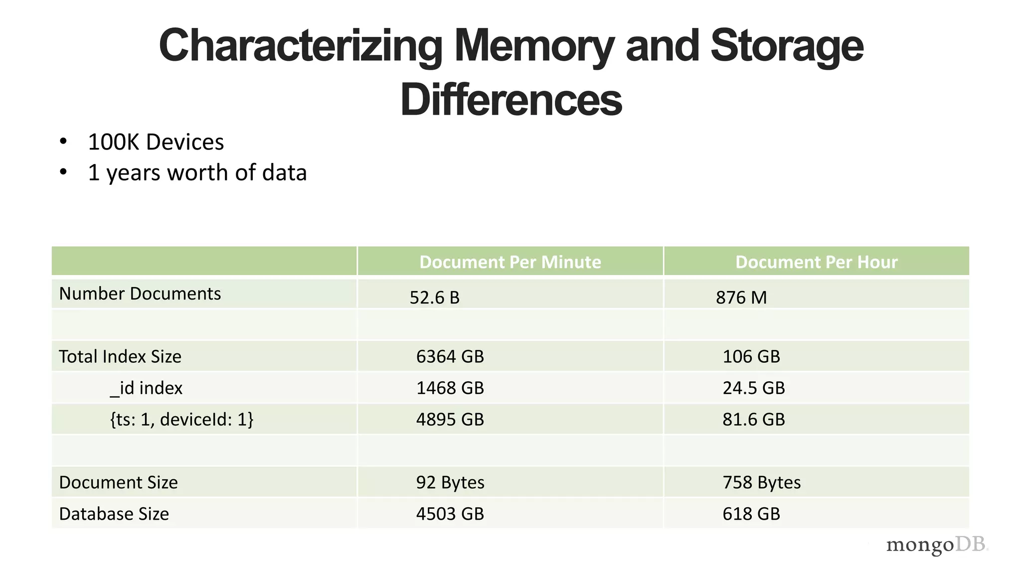
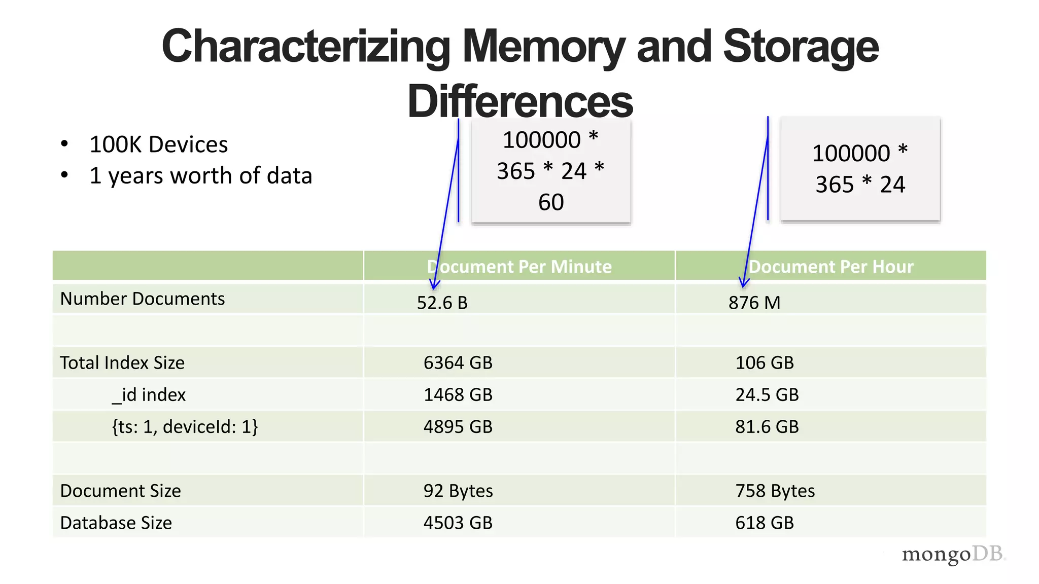
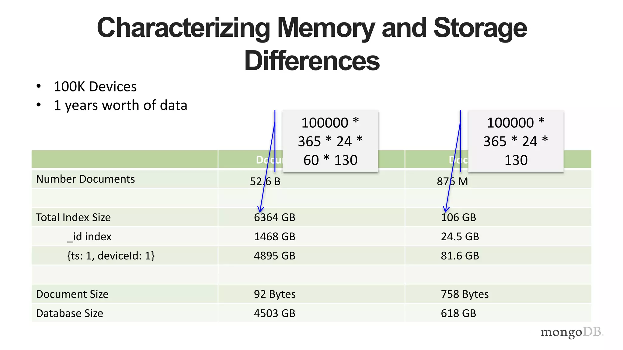
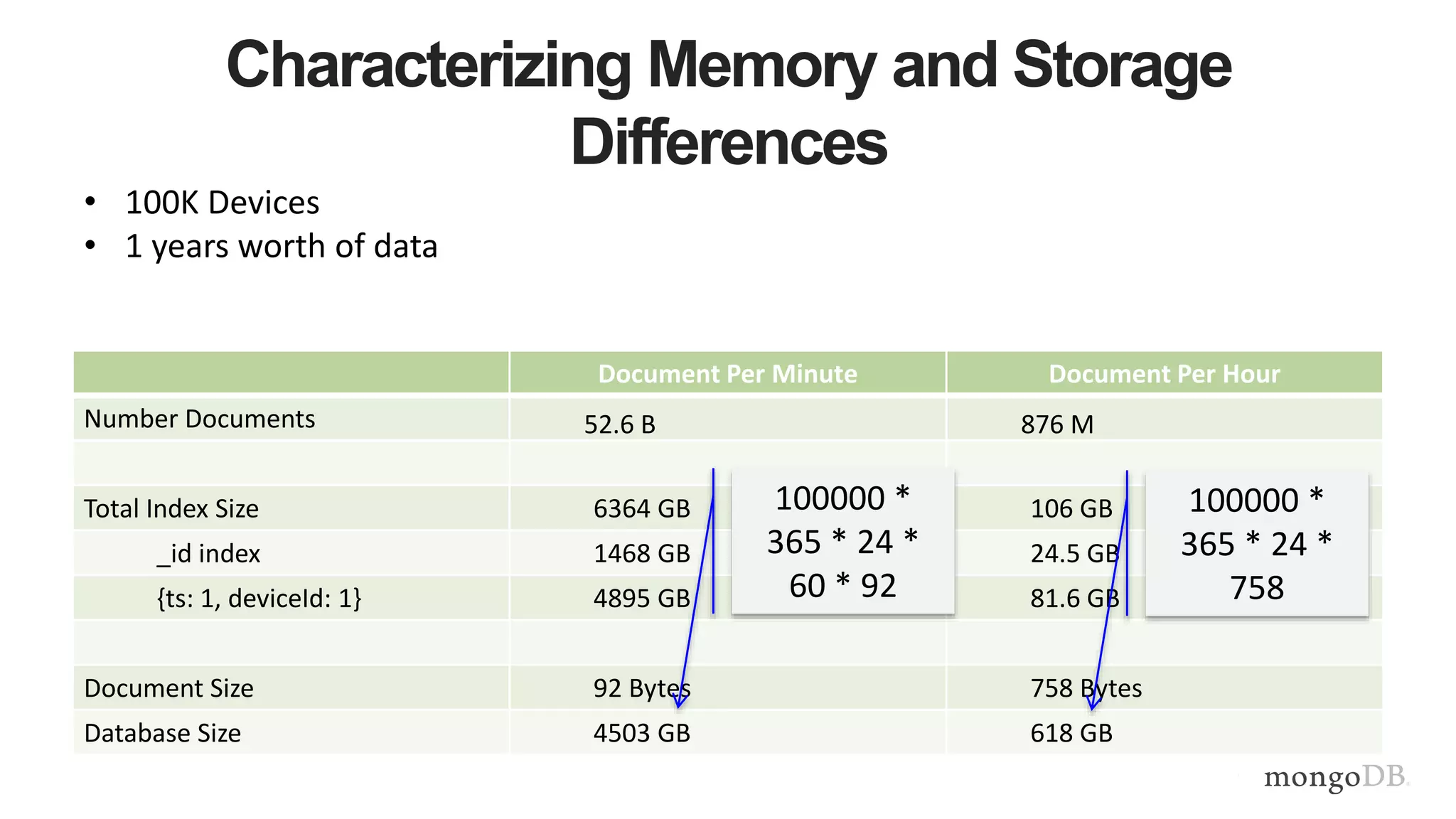

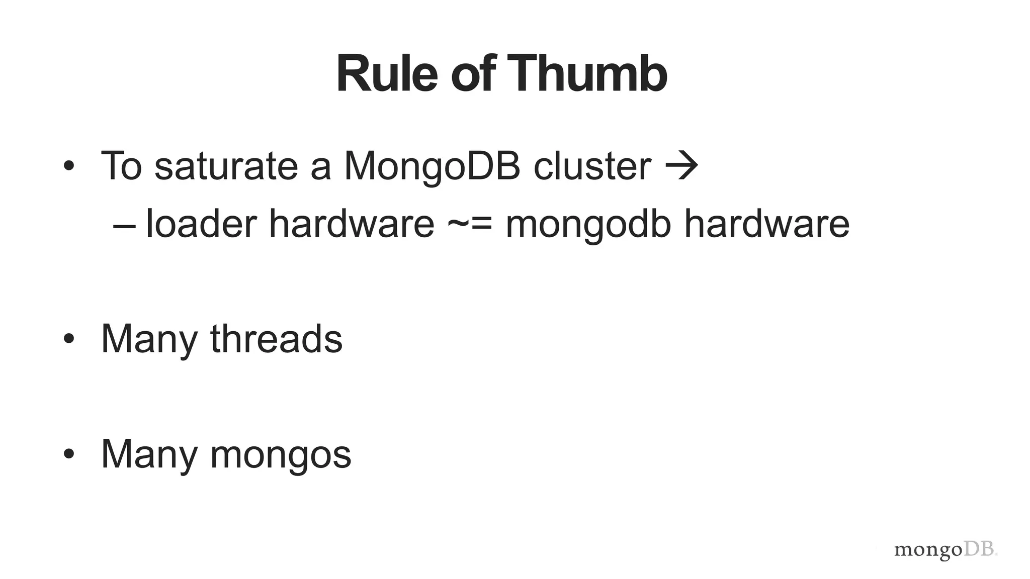


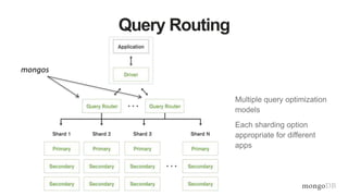
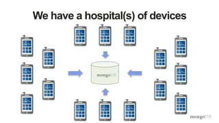
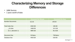
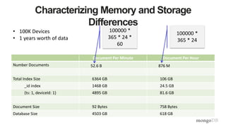
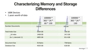
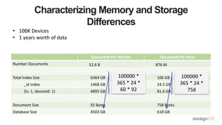
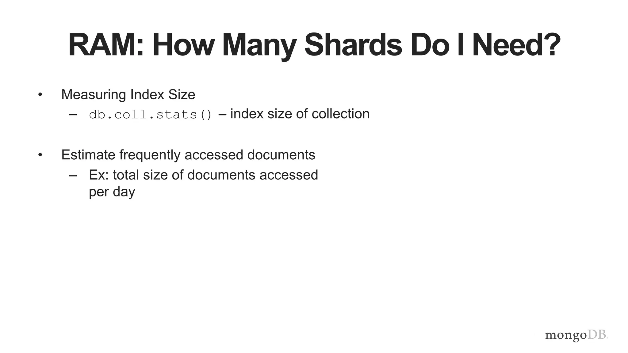
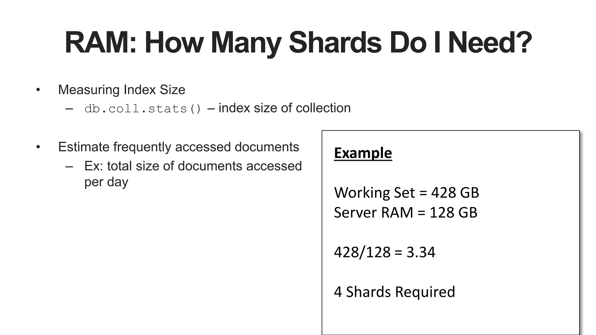
This document provides MongoDB best practices for schema design and data modeling. It discusses when to embed documents versus reference them, and how that impacts performance. It also uses an example of medical device data to illustrate how aggregating data at regular intervals (e.g. hourly instead of per minute) can significantly reduce storage requirements and improve query performance. Proper schema design is important for determining the required hardware resources.


![[JAWS DAYS 2019] Amazon DocumentDB(with MongoDB Compatibility)入門](https://cdn.slidesharecdn.com/ss_thumbnails/jawsdays-2019-190222234012-thumbnail.jpg?width=600ounds&width=560&fit=bounds)


