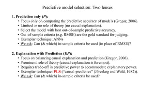
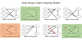
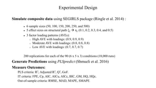
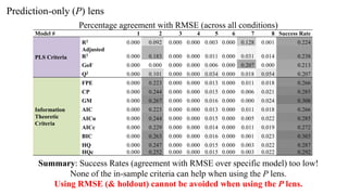
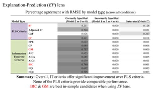
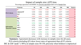
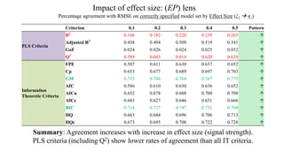
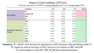
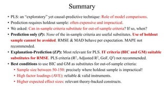
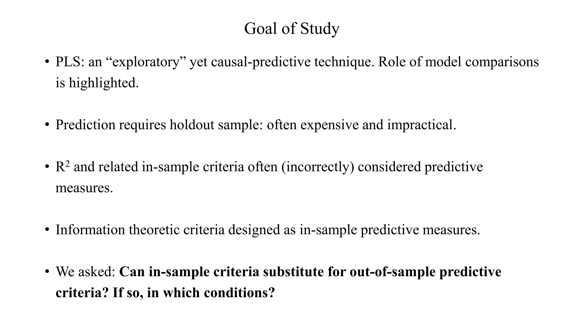
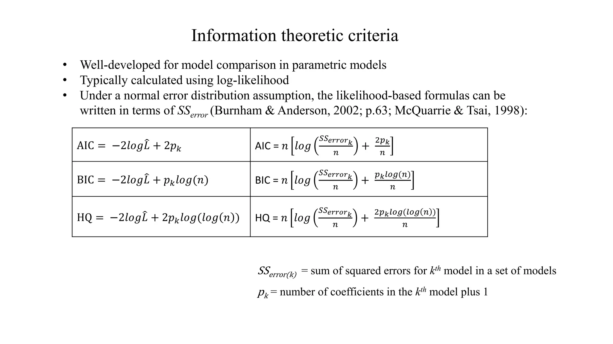
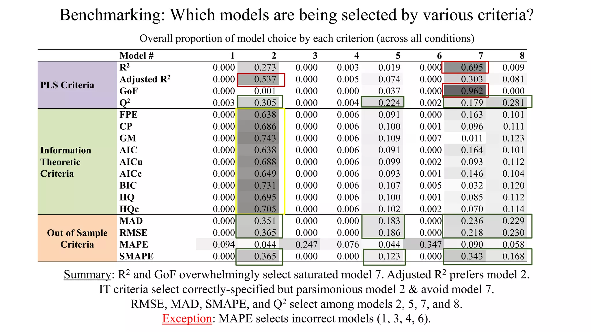
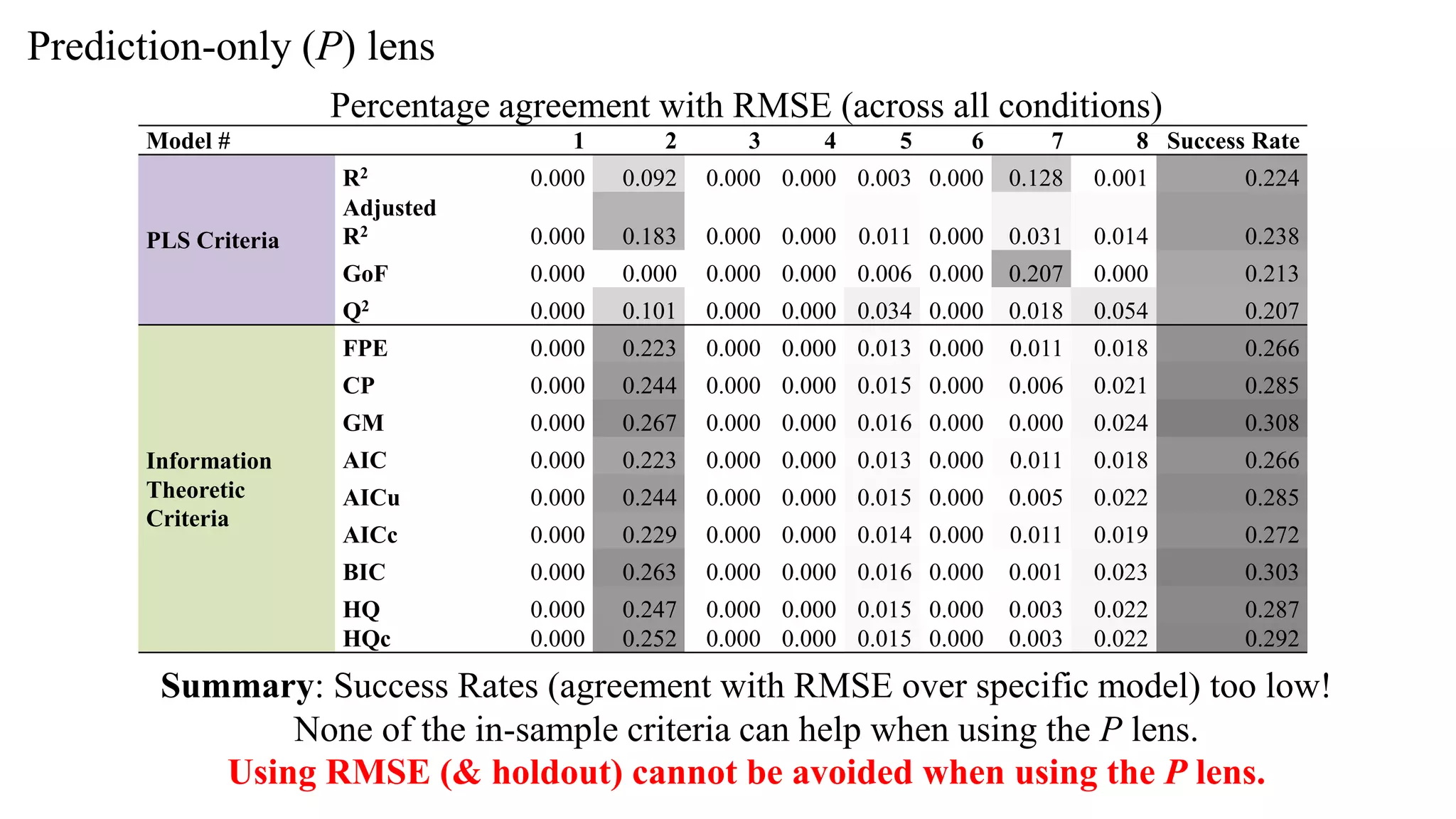
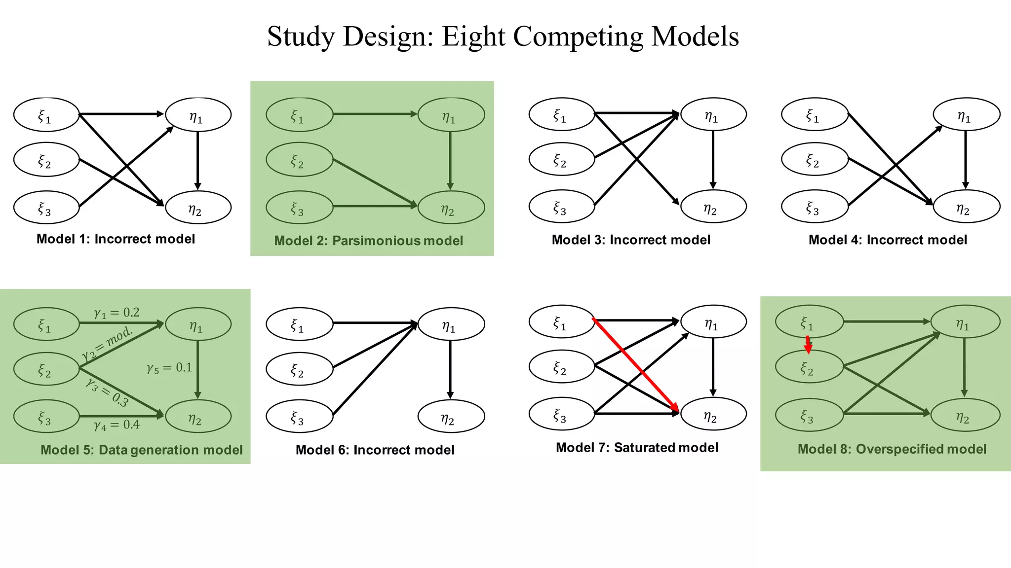
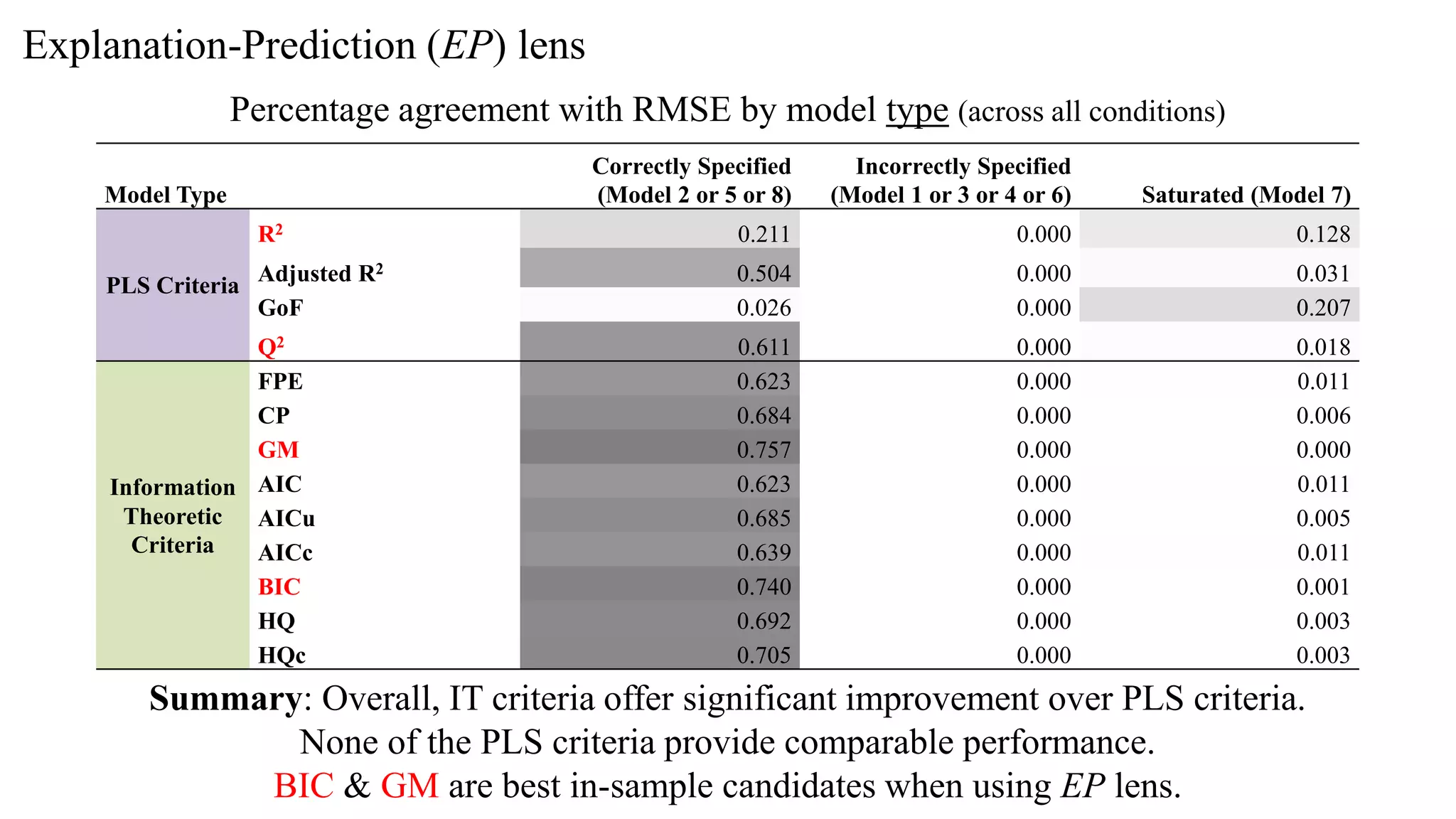
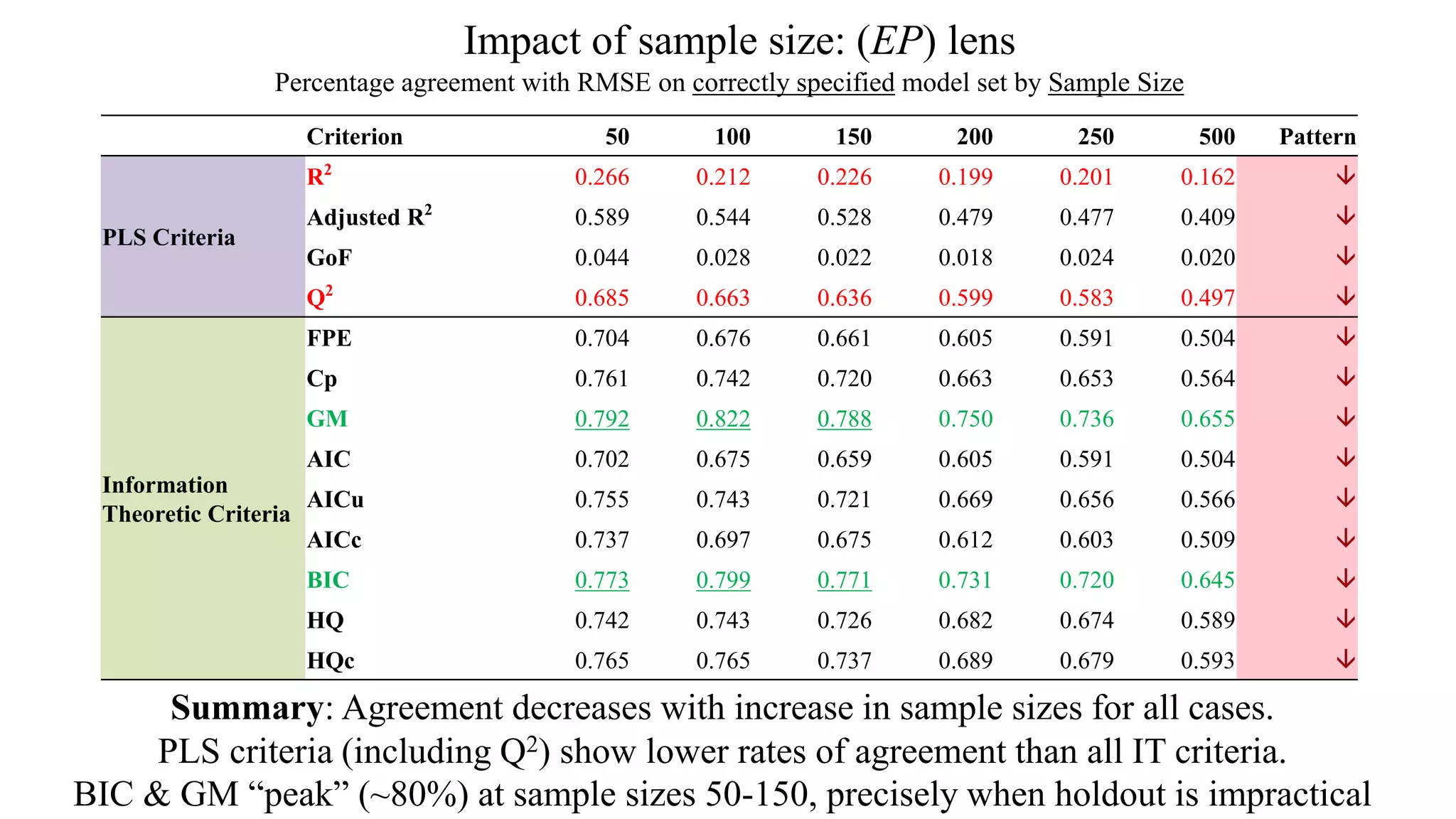
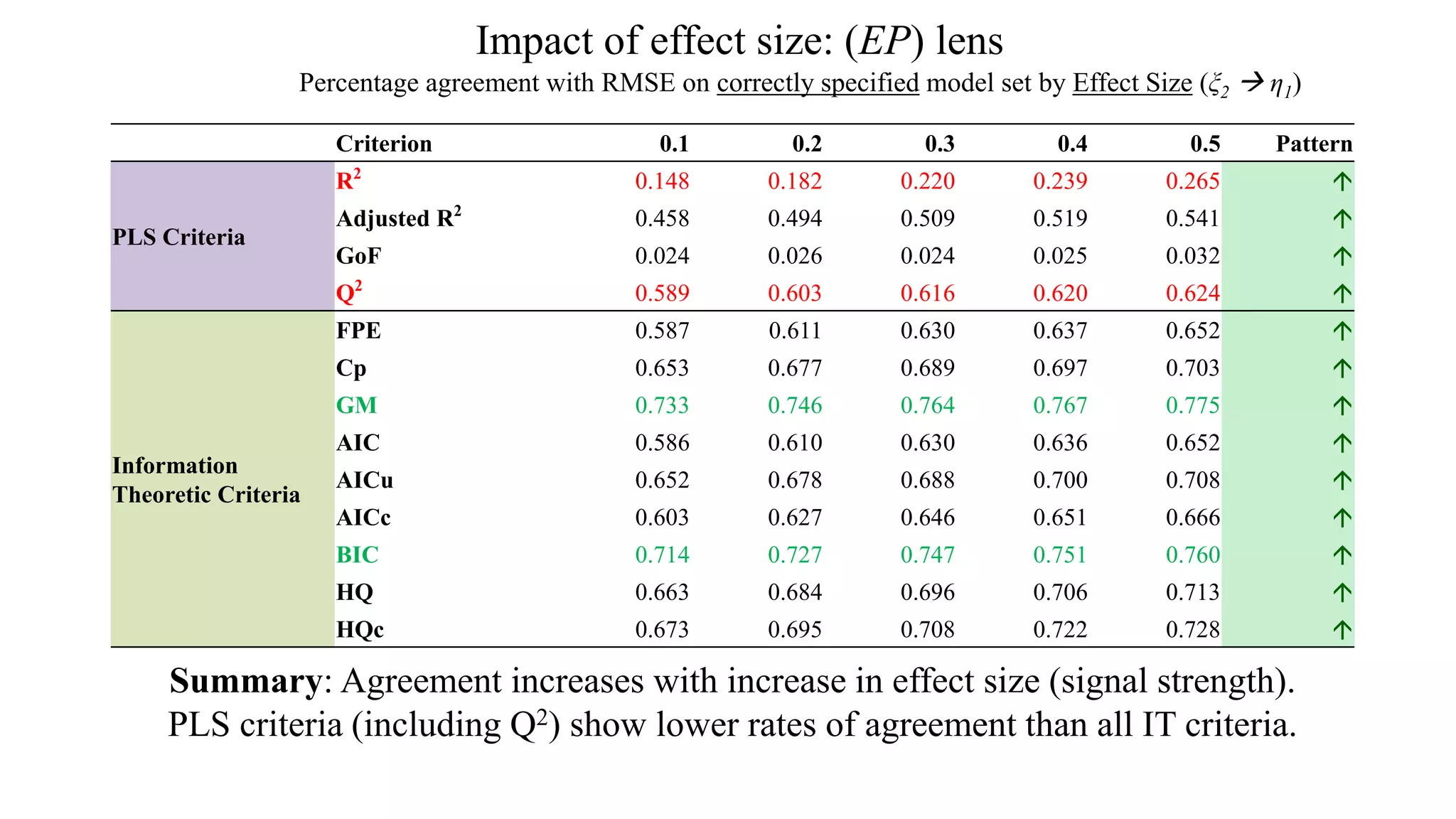
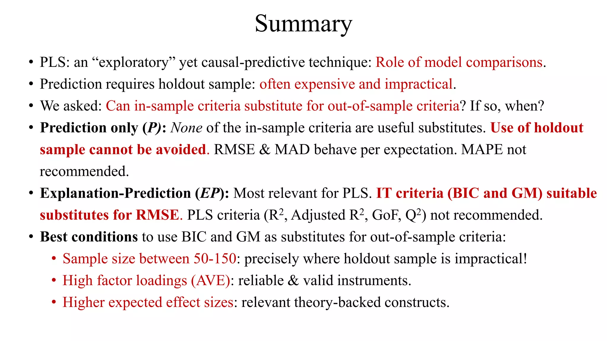
KEMBAR78
Prediction-based Model Selection in PLS-PM | PPTX
Prediction-oriented Model
Selection in PLS-PM
Pratyush Nidhi Sharma, University of Delaware
Galit Shmueli*, National Tsing Hua University
Marko Sarstedt, Otto-van-Guericke-University Magdeburg
Nicholas Danks, National Tsing Hua University
Soumya Ray, National Tsing Hua University
Goal of Study
• PLS: an “exploratory” yet causal-predictive technique. Role of model comparisons
is highlighted.
• Prediction requires holdout sample: often expensive and impractical.
• R2 and related in-sample criteria often (incorrectly) considered predictive
measures.
• Information theoretic criteria designed as in-sample predictive measures.
• We asked: Can in-sample criteria substitute for out-of-sample predictive
criteria? If so, in which conditions?
Information theoretic criteria
AIC = −2𝑙𝑜𝑔 𝐿 + 2𝑝 𝑘 AIC = 𝑛 𝑙𝑜𝑔
𝑆𝑆 𝑒𝑟𝑟𝑜𝑟 𝑘
𝑛
+
2𝑝 𝑘
𝑛
BIC = −2𝑙𝑜𝑔 𝐿 + 𝑝 𝑘 𝑙𝑜𝑔(𝑛) BIC = 𝑛 𝑙𝑜𝑔
𝑆𝑆 𝑒𝑟𝑟𝑜𝑟 𝑘
𝑛
+
𝑝 𝑘 𝑙𝑜𝑔(𝑛)
𝑛
HQ = −2𝑙𝑜𝑔 𝐿 + 2𝑝 𝑘 𝑙𝑜𝑔(𝑙𝑜𝑔 𝑛 ) HQ = 𝑛 𝑙𝑜𝑔
𝑆𝑆 𝑒𝑟𝑟𝑜𝑟 𝑘
𝑛
+
2𝑝 𝑘 𝑙𝑜𝑔(𝑙𝑜𝑔 𝑛 )
𝑛
SSerror(k) = sum of squared errors for kth model in a set of models
pk = number of coefficients in the kth model plus 1
• Well-developed for model comparison in parametric models
• Typically calculated using log-likelihood
• Under a normal error distribution assumption, the likelihood-based formulas can be
written in terms of SSerror (Burnham & Anderson, 2002; p.63; McQuarrie & Tsai, 1998):
Predictive model selection: Two lenses
1. Prediction only (P):
• Focus only on comparing the predictive accuracy of models (Gregor, 2006).
• Limited or no role of theory (no causal explanation).
• Select the model with best out-of-sample predictive accuracy.
• Out-of-sample criteria (e.g. RMSE) are the gold standard for judging.
• Exemplar technique: ANNs
• We ask: Can (& which) in-sample criteria be used (in place of RMSE)?
2. Explanation with Prediction (EP):
• Focus on balancing causal explanation and prediction (Gregor, 2006).
• Prominent role of theory (causal explanation is foremost).
• Requires trade-off in predictive power to accommodate explanatory power.
• Exemplar technique: PLS (“causal-predictive” (Jöreskog and Wold, 1982)).
• We ask: Can (& which) in-sample criteria be used?
Study Design: Eight Competing Models
Experimental Design
Simulate composite data using SEGIRLS package (Ringle et al. 2014) :
● 6 sample sizes (50, 100, 150, 200, 250, and 500)
● 5 effect sizes on structural path ξ2  η1 (0.1, 0.2, 0.3, 0.4, and 0.5)
● 3 factor loading patterns (AVEs):
o High AVE with loadings: (0.9, 0.9, 0.9)
o Moderate AVE with loadings: (0.8, 0.8, 0.8)
o Low AVE with loadings: (0.7, 0.7, 0.7)
200 replications for each of the 90 (6 x 5 x 3) conditions (18,000 runs)
Generate Predictions using PLSpredict (Shmueli et al. 2016)
Measure Outcomes:
PLS criteria: R2, Adjusted R2, Q2, GoF.
IT criteria: FPE, Cp, AIC, AICu, AICc, BIC, GM, HQ, HQc.
Out-of-sample criteria: RMSE, MAD, MAPE, SMAPE.
Procedure for assessing predictive model selection performance
Step # Details
1 Generate training & holdout data from data generating model (Model 5).
2 Estimate all 8 competing PLS models on the training data.
3 Compute the in-sample criteria for all 8 competing models using the training data.
4 Predict holdout items and compute out-of-sample criteria for all 8 competing models using
PLSPredict (Shmueli et al.’s 2016).
5 Compare the best model selected by each in-sample criterion to the RMSE-selected model.
Benchmarking: Which models are being selected by various criteria?
Overall proportion of model choice by each criterion (across all conditions)
Model # 1 2 3 4 5 6 7 8
PLS Criteria
R2 0.000 0.273 0.000 0.003 0.019 0.000 0.695 0.009
Adjusted R2 0.000 0.537 0.000 0.005 0.074 0.000 0.303 0.081
GoF 0.000 0.001 0.000 0.000 0.037 0.000 0.962 0.000
Q2 0.003 0.305 0.000 0.004 0.224 0.002 0.179 0.281
Information
Theoretic
Criteria
FPE 0.000 0.638 0.000 0.006 0.091 0.000 0.163 0.101
CP 0.000 0.686 0.000 0.006 0.100 0.001 0.096 0.111
GM 0.000 0.743 0.000 0.006 0.109 0.007 0.011 0.123
AIC 0.000 0.638 0.000 0.006 0.091 0.000 0.164 0.101
AICu 0.000 0.688 0.000 0.006 0.099 0.002 0.093 0.112
AICc 0.000 0.649 0.000 0.006 0.093 0.001 0.146 0.104
BIC 0.000 0.731 0.000 0.006 0.107 0.005 0.032 0.120
HQ 0.000 0.695 0.000 0.006 0.100 0.001 0.085 0.112
HQc 0.000 0.705 0.000 0.006 0.102 0.002 0.070 0.114
Out of Sample
Criteria
MAD 0.000 0.351 0.000 0.000 0.183 0.000 0.236 0.229
RMSE 0.000 0.365 0.000 0.000 0.186 0.000 0.218 0.230
MAPE 0.094 0.044 0.247 0.076 0.044 0.347 0.090 0.058
SMAPE 0.000 0.365 0.000 0.000 0.123 0.000 0.343 0.168
Summary: R2 and GoF overwhelmingly select saturated model 7. Adjusted R2 prefers model 2.
IT criteria select correctly-specified but parsimonious model 2 & avoid model 7.
RMSE, MAD, SMAPE, and Q2 select among models 2, 5, 7, and 8.
Exception: MAPE selects incorrect models (1, 3, 4, 6).
Assessing the performance in the P lens
Can (& which) in-sample criteria help select the
best predictive model?
(regardless of correct specification)
Prediction-only (P) lens
Percentage agreement with RMSE (across all conditions)
Model # 1 2 3 4 5 6 7 8 Success Rate
PLS Criteria
R2 0.000 0.092 0.000 0.000 0.003 0.000 0.128 0.001 0.224
Adjusted
R2 0.000 0.183 0.000 0.000 0.011 0.000 0.031 0.014 0.238
GoF 0.000 0.000 0.000 0.000 0.006 0.000 0.207 0.000 0.213
Q2 0.000 0.101 0.000 0.000 0.034 0.000 0.018 0.054 0.207
Information
Theoretic
Criteria
FPE 0.000 0.223 0.000 0.000 0.013 0.000 0.011 0.018 0.266
CP 0.000 0.244 0.000 0.000 0.015 0.000 0.006 0.021 0.285
GM 0.000 0.267 0.000 0.000 0.016 0.000 0.000 0.024 0.308
AIC 0.000 0.223 0.000 0.000 0.013 0.000 0.011 0.018 0.266
AICu 0.000 0.244 0.000 0.000 0.015 0.000 0.005 0.022 0.285
AICc 0.000 0.229 0.000 0.000 0.014 0.000 0.011 0.019 0.272
BIC 0.000 0.263 0.000 0.000 0.016 0.000 0.001 0.023 0.303
HQ 0.000 0.247 0.000 0.000 0.015 0.000 0.003 0.022 0.287
HQc 0.000 0.252 0.000 0.000 0.015 0.000 0.003 0.022 0.292
Summary: Success Rates (agreement with RMSE over specific model) too low!
None of the in-sample criteria can help when using the P lens.
Using RMSE (& holdout) cannot be avoided when using the P lens.
Assessing the performance in the EP lens
Can (& which) in-sample criteria help select a
correctly specified (w.r.t. η2)
but highly predictive model?
Study Design: Eight Competing Models
Explanation-Prediction (EP) lens
Percentage agreement with RMSE by model type (across all conditions)
Model Type
Correctly Specified
(Model 2 or 5 or 8)
Incorrectly Specified
(Model 1 or 3 or 4 or 6) Saturated (Model 7)
PLS Criteria
R2 0.211 0.000 0.128
Adjusted R2 0.504 0.000 0.031
GoF 0.026 0.000 0.207
Q2 0.611 0.000 0.018
Information
Theoretic
Criteria
FPE 0.623 0.000 0.011
CP 0.684 0.000 0.006
GM 0.757 0.000 0.000
AIC 0.623 0.000 0.011
AICu 0.685 0.000 0.005
AICc 0.639 0.000 0.011
BIC 0.740 0.000 0.001
HQ 0.692 0.000 0.003
HQc 0.705 0.000 0.003
Summary: Overall, IT criteria offer significant improvement over PLS criteria.
None of the PLS criteria provide comparable performance.
BIC & GM are best in-sample candidates when using EP lens.
How do experimental conditions affect model
selection in the EP lens?
Impact of sample size: (EP) lens
Percentage agreement with RMSE on correctly specified model set by Sample Size
Criterion 50 100 150 200 250 500 Pattern
PLS Criteria
R2
0.266 0.212 0.226 0.199 0.201 0.162 
Adjusted R2
0.589 0.544 0.528 0.479 0.477 0.409 
GoF 0.044 0.028 0.022 0.018 0.024 0.020 
Q2
0.685 0.663 0.636 0.599 0.583 0.497 
Information
Theoretic Criteria
FPE 0.704 0.676 0.661 0.605 0.591 0.504 
Cp 0.761 0.742 0.720 0.663 0.653 0.564 
GM 0.792 0.822 0.788 0.750 0.736 0.655 
AIC 0.702 0.675 0.659 0.605 0.591 0.504 
AICu 0.755 0.743 0.721 0.669 0.656 0.566 
AICc 0.737 0.697 0.675 0.612 0.603 0.509 
BIC 0.773 0.799 0.771 0.731 0.720 0.645 
HQ 0.742 0.743 0.726 0.682 0.674 0.589 
HQc 0.765 0.765 0.737 0.689 0.679 0.593 
Summary: Agreement decreases with increase in sample sizes for all cases.
PLS criteria (including Q2) show lower rates of agreement than all IT criteria.
BIC & GM “peak” (~80%) at sample sizes 50-150, precisely when holdout is impractical
Impact of effect size: (EP) lens
Percentage agreement with RMSE on correctly specified model set by Effect Size (ξ2  η1)
Criterion 0.1 0.2 0.3 0.4 0.5 Pattern
PLS Criteria
R2
0.148 0.182 0.220 0.239 0.265 
Adjusted R2
0.458 0.494 0.509 0.519 0.541 
GoF 0.024 0.026 0.024 0.025 0.032 
Q2
0.589 0.603 0.616 0.620 0.624 
Information
Theoretic Criteria
FPE 0.587 0.611 0.630 0.637 0.652 
Cp 0.653 0.677 0.689 0.697 0.703 
GM 0.733 0.746 0.764 0.767 0.775 
AIC 0.586 0.610 0.630 0.636 0.652 
AICu 0.652 0.678 0.688 0.700 0.708 
AICc 0.603 0.627 0.646 0.651 0.666 
BIC 0.714 0.727 0.747 0.751 0.760 
HQ 0.663 0.684 0.696 0.706 0.713 
HQc 0.673 0.695 0.708 0.722 0.728 
Summary: Agreement increases with increase in effect size (signal strength).
PLS criteria (including Q2) show lower rates of agreement than all IT criteria.
Impact of item loadings: (EP) lens
Percentage agreement with RMSE on correctly specified model set by Loading Values (AVE)
Criterion 0.7 0.8 0.9 Pattern
PLS Criteria
R2
0.264 0.218 0.152 
Adjusted R2
0.504 0.510 0.499 
GoF 0.038 0.026 0.014 
Q2
0.603 0.610 0.618 
Information Theoretic
Criteria
FPE 0.606 0.626 0.639 
Cp 0.648 0.688 0.716 
GM 0.726 0.762 0.784 
AIC 0.605 0.625 0.639 
AICu 0.658 0.689 0.708 
AICc 0.619 0.641 0.656 
BIC 0.708 0.744 0.767 
HQ 0.666 0.696 0.716 
HQc 0.678 0.708 0.729 
Summary: R2, Adj-R2, GoF decrease in agreement as AVE increases (start preferring model 7)
Q2 improves with an increase in AVE; however it is inferior to BIC and GM.
IT criteria improve with AVE; BIC & GM show best performance.
Summary
• PLS: an “exploratory” yet causal-predictive technique: Role of model comparisons.
• Prediction requires holdout sample: often expensive and impractical.
• We asked: Can in-sample criteria substitute for out-of-sample criteria? If so, when?
• Prediction only (P): None of the in-sample criteria are useful substitutes. Use of holdout
sample cannot be avoided. RMSE & MAD behave per expectation. MAPE not
recommended.
• Explanation-Prediction (EP): Most relevant for PLS. IT criteria (BIC and GM) suitable
substitutes for RMSE. PLS criteria (R2, Adjusted R2, GoF, Q2) not recommended.
• Best conditions to use BIC and GM as substitutes for out-of-sample criteria:
• Sample size between 50-150: precisely where holdout sample is impractical!
• High factor loadings (AVE): reliable & valid instruments.
• Higher expected effect sizes: relevant theory-backed constructs.
Robustness check!
What if the data generation model is not included in the
competing model set-up?
We introduce: Data generating Model X with hidden variable ξ4. Model X is out of reach!
• Results almost perfectly mimic the earlier (main) results.
• Conclusion: BIC & GM provide best predictive model selection ability regardless
of whether data generation is included or excluded (out of reach)!
• PLS criteria (R2, Adjusted R2, GoF, Q2) are not recommended.
Thank you!

Prediction-based Model Selection in PLS-PM

  • 1.
    Prediction-oriented Model Selection inPLS-PM Pratyush Nidhi Sharma, University of Delaware Galit Shmueli*, National Tsing Hua University Marko Sarstedt, Otto-van-Guericke-University Magdeburg Nicholas Danks, National Tsing Hua University Soumya Ray, National Tsing Hua University
  • 2.
    Goal of Study •PLS: an “exploratory” yet causal-predictive technique. Role of model comparisons is highlighted. • Prediction requires holdout sample: often expensive and impractical. • R2 and related in-sample criteria often (incorrectly) considered predictive measures. • Information theoretic criteria designed as in-sample predictive measures. • We asked: Can in-sample criteria substitute for out-of-sample predictive criteria? If so, in which conditions?
  • 3.
    Information theoretic criteria AIC= −2𝑙𝑜𝑔 𝐿 + 2𝑝 𝑘 AIC = 𝑛 𝑙𝑜𝑔 𝑆𝑆 𝑒𝑟𝑟𝑜𝑟 𝑘 𝑛 + 2𝑝 𝑘 𝑛 BIC = −2𝑙𝑜𝑔 𝐿 + 𝑝 𝑘 𝑙𝑜𝑔(𝑛) BIC = 𝑛 𝑙𝑜𝑔 𝑆𝑆 𝑒𝑟𝑟𝑜𝑟 𝑘 𝑛 + 𝑝 𝑘 𝑙𝑜𝑔(𝑛) 𝑛 HQ = −2𝑙𝑜𝑔 𝐿 + 2𝑝 𝑘 𝑙𝑜𝑔(𝑙𝑜𝑔 𝑛 ) HQ = 𝑛 𝑙𝑜𝑔 𝑆𝑆 𝑒𝑟𝑟𝑜𝑟 𝑘 𝑛 + 2𝑝 𝑘 𝑙𝑜𝑔(𝑙𝑜𝑔 𝑛 ) 𝑛 SSerror(k) = sum of squared errors for kth model in a set of models pk = number of coefficients in the kth model plus 1 • Well-developed for model comparison in parametric models • Typically calculated using log-likelihood • Under a normal error distribution assumption, the likelihood-based formulas can be written in terms of SSerror (Burnham & Anderson, 2002; p.63; McQuarrie & Tsai, 1998):
  • 4.
    Predictive model selection:Two lenses 1. Prediction only (P): • Focus only on comparing the predictive accuracy of models (Gregor, 2006). • Limited or no role of theory (no causal explanation). • Select the model with best out-of-sample predictive accuracy. • Out-of-sample criteria (e.g. RMSE) are the gold standard for judging. • Exemplar technique: ANNs • We ask: Can (& which) in-sample criteria be used (in place of RMSE)? 2. Explanation with Prediction (EP): • Focus on balancing causal explanation and prediction (Gregor, 2006). • Prominent role of theory (causal explanation is foremost). • Requires trade-off in predictive power to accommodate explanatory power. • Exemplar technique: PLS (“causal-predictive” (Jöreskog and Wold, 1982)). • We ask: Can (& which) in-sample criteria be used?
  • 5.
    Study Design: EightCompeting Models
  • 6.
    Experimental Design Simulate compositedata using SEGIRLS package (Ringle et al. 2014) : ● 6 sample sizes (50, 100, 150, 200, 250, and 500) ● 5 effect sizes on structural path ξ2  η1 (0.1, 0.2, 0.3, 0.4, and 0.5) ● 3 factor loading patterns (AVEs): o High AVE with loadings: (0.9, 0.9, 0.9) o Moderate AVE with loadings: (0.8, 0.8, 0.8) o Low AVE with loadings: (0.7, 0.7, 0.7) 200 replications for each of the 90 (6 x 5 x 3) conditions (18,000 runs) Generate Predictions using PLSpredict (Shmueli et al. 2016) Measure Outcomes: PLS criteria: R2, Adjusted R2, Q2, GoF. IT criteria: FPE, Cp, AIC, AICu, AICc, BIC, GM, HQ, HQc. Out-of-sample criteria: RMSE, MAD, MAPE, SMAPE.
  • 7.
    Procedure for assessingpredictive model selection performance Step # Details 1 Generate training & holdout data from data generating model (Model 5). 2 Estimate all 8 competing PLS models on the training data. 3 Compute the in-sample criteria for all 8 competing models using the training data. 4 Predict holdout items and compute out-of-sample criteria for all 8 competing models using PLSPredict (Shmueli et al.’s 2016). 5 Compare the best model selected by each in-sample criterion to the RMSE-selected model.
  • 9.
    Benchmarking: Which modelsare being selected by various criteria? Overall proportion of model choice by each criterion (across all conditions) Model # 1 2 3 4 5 6 7 8 PLS Criteria R2 0.000 0.273 0.000 0.003 0.019 0.000 0.695 0.009 Adjusted R2 0.000 0.537 0.000 0.005 0.074 0.000 0.303 0.081 GoF 0.000 0.001 0.000 0.000 0.037 0.000 0.962 0.000 Q2 0.003 0.305 0.000 0.004 0.224 0.002 0.179 0.281 Information Theoretic Criteria FPE 0.000 0.638 0.000 0.006 0.091 0.000 0.163 0.101 CP 0.000 0.686 0.000 0.006 0.100 0.001 0.096 0.111 GM 0.000 0.743 0.000 0.006 0.109 0.007 0.011 0.123 AIC 0.000 0.638 0.000 0.006 0.091 0.000 0.164 0.101 AICu 0.000 0.688 0.000 0.006 0.099 0.002 0.093 0.112 AICc 0.000 0.649 0.000 0.006 0.093 0.001 0.146 0.104 BIC 0.000 0.731 0.000 0.006 0.107 0.005 0.032 0.120 HQ 0.000 0.695 0.000 0.006 0.100 0.001 0.085 0.112 HQc 0.000 0.705 0.000 0.006 0.102 0.002 0.070 0.114 Out of Sample Criteria MAD 0.000 0.351 0.000 0.000 0.183 0.000 0.236 0.229 RMSE 0.000 0.365 0.000 0.000 0.186 0.000 0.218 0.230 MAPE 0.094 0.044 0.247 0.076 0.044 0.347 0.090 0.058 SMAPE 0.000 0.365 0.000 0.000 0.123 0.000 0.343 0.168 Summary: R2 and GoF overwhelmingly select saturated model 7. Adjusted R2 prefers model 2. IT criteria select correctly-specified but parsimonious model 2 & avoid model 7. RMSE, MAD, SMAPE, and Q2 select among models 2, 5, 7, and 8. Exception: MAPE selects incorrect models (1, 3, 4, 6).
  • 10.
    Assessing the performancein the P lens Can (& which) in-sample criteria help select the best predictive model? (regardless of correct specification)
  • 11.
    Prediction-only (P) lens Percentageagreement with RMSE (across all conditions) Model # 1 2 3 4 5 6 7 8 Success Rate PLS Criteria R2 0.000 0.092 0.000 0.000 0.003 0.000 0.128 0.001 0.224 Adjusted R2 0.000 0.183 0.000 0.000 0.011 0.000 0.031 0.014 0.238 GoF 0.000 0.000 0.000 0.000 0.006 0.000 0.207 0.000 0.213 Q2 0.000 0.101 0.000 0.000 0.034 0.000 0.018 0.054 0.207 Information Theoretic Criteria FPE 0.000 0.223 0.000 0.000 0.013 0.000 0.011 0.018 0.266 CP 0.000 0.244 0.000 0.000 0.015 0.000 0.006 0.021 0.285 GM 0.000 0.267 0.000 0.000 0.016 0.000 0.000 0.024 0.308 AIC 0.000 0.223 0.000 0.000 0.013 0.000 0.011 0.018 0.266 AICu 0.000 0.244 0.000 0.000 0.015 0.000 0.005 0.022 0.285 AICc 0.000 0.229 0.000 0.000 0.014 0.000 0.011 0.019 0.272 BIC 0.000 0.263 0.000 0.000 0.016 0.000 0.001 0.023 0.303 HQ 0.000 0.247 0.000 0.000 0.015 0.000 0.003 0.022 0.287 HQc 0.000 0.252 0.000 0.000 0.015 0.000 0.003 0.022 0.292 Summary: Success Rates (agreement with RMSE over specific model) too low! None of the in-sample criteria can help when using the P lens. Using RMSE (& holdout) cannot be avoided when using the P lens.
  • 12.
    Assessing the performancein the EP lens Can (& which) in-sample criteria help select a correctly specified (w.r.t. η2) but highly predictive model?
  • 13.
    Study Design: EightCompeting Models
  • 14.
    Explanation-Prediction (EP) lens Percentageagreement with RMSE by model type (across all conditions) Model Type Correctly Specified (Model 2 or 5 or 8) Incorrectly Specified (Model 1 or 3 or 4 or 6) Saturated (Model 7) PLS Criteria R2 0.211 0.000 0.128 Adjusted R2 0.504 0.000 0.031 GoF 0.026 0.000 0.207 Q2 0.611 0.000 0.018 Information Theoretic Criteria FPE 0.623 0.000 0.011 CP 0.684 0.000 0.006 GM 0.757 0.000 0.000 AIC 0.623 0.000 0.011 AICu 0.685 0.000 0.005 AICc 0.639 0.000 0.011 BIC 0.740 0.000 0.001 HQ 0.692 0.000 0.003 HQc 0.705 0.000 0.003 Summary: Overall, IT criteria offer significant improvement over PLS criteria. None of the PLS criteria provide comparable performance. BIC & GM are best in-sample candidates when using EP lens.
  • 15.
    How do experimentalconditions affect model selection in the EP lens?
  • 16.
    Impact of samplesize: (EP) lens Percentage agreement with RMSE on correctly specified model set by Sample Size Criterion 50 100 150 200 250 500 Pattern PLS Criteria R2 0.266 0.212 0.226 0.199 0.201 0.162  Adjusted R2 0.589 0.544 0.528 0.479 0.477 0.409  GoF 0.044 0.028 0.022 0.018 0.024 0.020  Q2 0.685 0.663 0.636 0.599 0.583 0.497  Information Theoretic Criteria FPE 0.704 0.676 0.661 0.605 0.591 0.504  Cp 0.761 0.742 0.720 0.663 0.653 0.564  GM 0.792 0.822 0.788 0.750 0.736 0.655  AIC 0.702 0.675 0.659 0.605 0.591 0.504  AICu 0.755 0.743 0.721 0.669 0.656 0.566  AICc 0.737 0.697 0.675 0.612 0.603 0.509  BIC 0.773 0.799 0.771 0.731 0.720 0.645  HQ 0.742 0.743 0.726 0.682 0.674 0.589  HQc 0.765 0.765 0.737 0.689 0.679 0.593  Summary: Agreement decreases with increase in sample sizes for all cases. PLS criteria (including Q2) show lower rates of agreement than all IT criteria. BIC & GM “peak” (~80%) at sample sizes 50-150, precisely when holdout is impractical
  • 17.
    Impact of effectsize: (EP) lens Percentage agreement with RMSE on correctly specified model set by Effect Size (ξ2  η1) Criterion 0.1 0.2 0.3 0.4 0.5 Pattern PLS Criteria R2 0.148 0.182 0.220 0.239 0.265  Adjusted R2 0.458 0.494 0.509 0.519 0.541  GoF 0.024 0.026 0.024 0.025 0.032  Q2 0.589 0.603 0.616 0.620 0.624  Information Theoretic Criteria FPE 0.587 0.611 0.630 0.637 0.652  Cp 0.653 0.677 0.689 0.697 0.703  GM 0.733 0.746 0.764 0.767 0.775  AIC 0.586 0.610 0.630 0.636 0.652  AICu 0.652 0.678 0.688 0.700 0.708  AICc 0.603 0.627 0.646 0.651 0.666  BIC 0.714 0.727 0.747 0.751 0.760  HQ 0.663 0.684 0.696 0.706 0.713  HQc 0.673 0.695 0.708 0.722 0.728  Summary: Agreement increases with increase in effect size (signal strength). PLS criteria (including Q2) show lower rates of agreement than all IT criteria.
  • 18.
    Impact of itemloadings: (EP) lens Percentage agreement with RMSE on correctly specified model set by Loading Values (AVE) Criterion 0.7 0.8 0.9 Pattern PLS Criteria R2 0.264 0.218 0.152  Adjusted R2 0.504 0.510 0.499  GoF 0.038 0.026 0.014  Q2 0.603 0.610 0.618  Information Theoretic Criteria FPE 0.606 0.626 0.639  Cp 0.648 0.688 0.716  GM 0.726 0.762 0.784  AIC 0.605 0.625 0.639  AICu 0.658 0.689 0.708  AICc 0.619 0.641 0.656  BIC 0.708 0.744 0.767  HQ 0.666 0.696 0.716  HQc 0.678 0.708 0.729  Summary: R2, Adj-R2, GoF decrease in agreement as AVE increases (start preferring model 7) Q2 improves with an increase in AVE; however it is inferior to BIC and GM. IT criteria improve with AVE; BIC & GM show best performance.
  • 19.
    Summary • PLS: an“exploratory” yet causal-predictive technique: Role of model comparisons. • Prediction requires holdout sample: often expensive and impractical. • We asked: Can in-sample criteria substitute for out-of-sample criteria? If so, when? • Prediction only (P): None of the in-sample criteria are useful substitutes. Use of holdout sample cannot be avoided. RMSE & MAD behave per expectation. MAPE not recommended. • Explanation-Prediction (EP): Most relevant for PLS. IT criteria (BIC and GM) suitable substitutes for RMSE. PLS criteria (R2, Adjusted R2, GoF, Q2) not recommended. • Best conditions to use BIC and GM as substitutes for out-of-sample criteria: • Sample size between 50-150: precisely where holdout sample is impractical! • High factor loadings (AVE): reliable & valid instruments. • Higher expected effect sizes: relevant theory-backed constructs.
  • 20.
    Robustness check! What ifthe data generation model is not included in the competing model set-up? We introduce: Data generating Model X with hidden variable ξ4. Model X is out of reach! • Results almost perfectly mimic the earlier (main) results. • Conclusion: BIC & GM provide best predictive model selection ability regardless of whether data generation is included or excluded (out of reach)! • PLS criteria (R2, Adjusted R2, GoF, Q2) are not recommended.
  • 21.