Introduction
A classifieris used to predict an outcome of a test data
Such a prediction is useful in many applications
Business forecasting, cause-and-effect analysis, etc.
A number of classifiers have been evolved to support the activities.
Each has their own merits and demerits
There is a need to estimate the accuracy and performance of the classifier with
respect to few controlling parameters in data sensitivity
As a task of sensitivity analysis, we have to focus on
Estimation strategy
Metrics for measuring accuracy
Metrics for measuring performance 3
Planning for Estimation
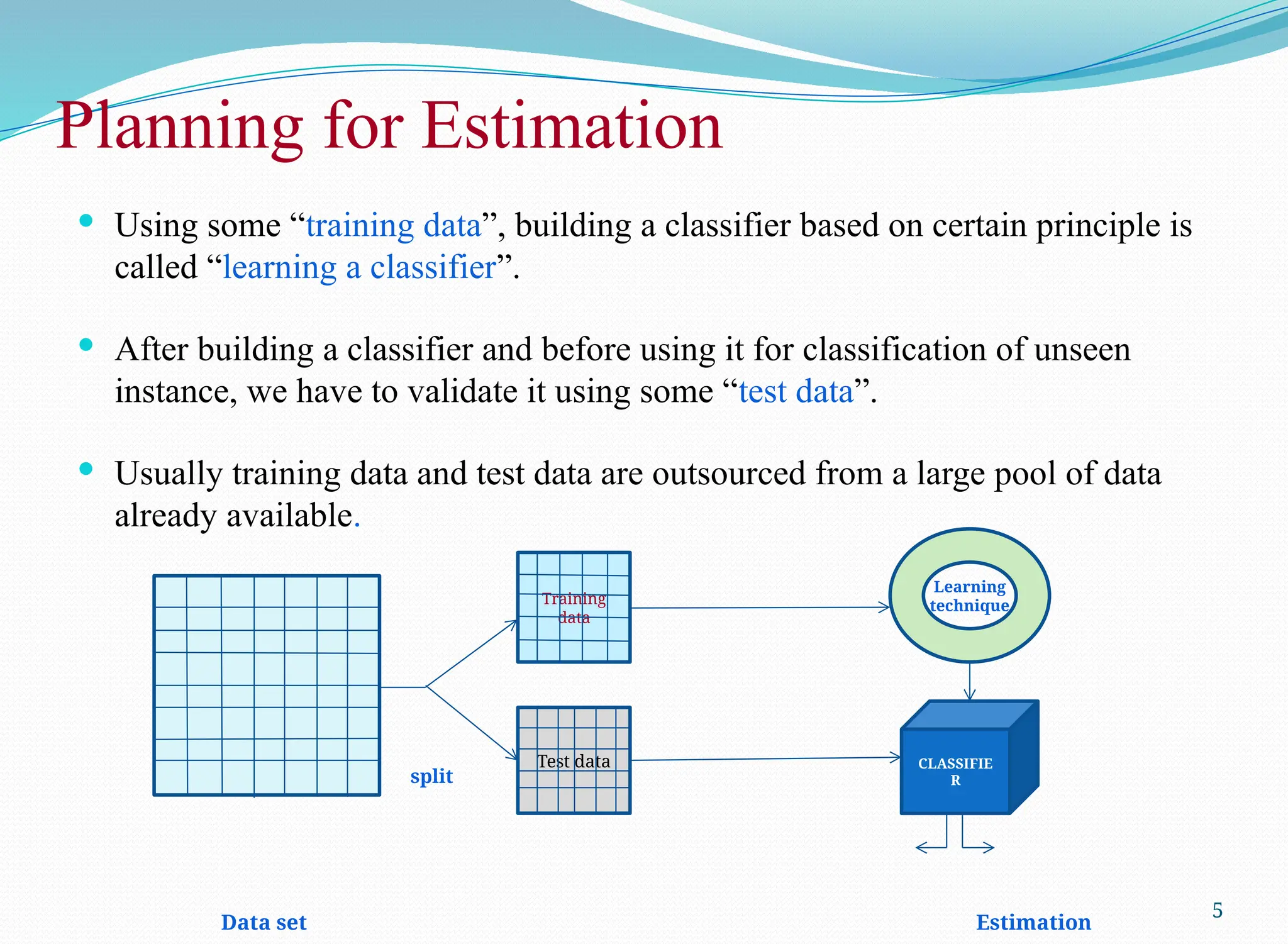
Using some “training data”, building a classifier based on certain principle is
called “learning a classifier”.
After building a classifier and before using it for classification of unseen
instance, we have to validate it using some “test data”.
Usually training data and test data are outsourced from a large pool of data
already available.
split
Data set Estimation
5
Training
data
Test data
Learning
technique
CLASSIFIE
R
6.
Estimation Strategies
Accuracyand performance measurement should follow a strategy.
As the topic is important, many strategies have been advocated so
far. Most widely used strategies are
Holdout method
Random subsampling
Cross-validation
Bootstrap approach
6
7.
Holdout Method
Thisis a basic concept of estimating a prediction.
Given a dataset, it is partitioned into two disjoint sets called training set and
testing set.
Classifier is learned based on the training set and get evaluated with testing set.
Proportion of training and testing sets is at the discretion of analyst; typically
1:1 or 2:1, and there is a trade-off between these sizes of these two sets.
If the training set is too large, then model may be good enough, but estimation
may be less reliable due to small testing set and vice-versa.
7
8.
Random Subsampling
Itis a variation of Holdout method to overcome the drawback of over-
presenting a class in one set thus under-presenting it in the other set and
vice-versa.
In this method, Holdout method is repeated k times, and in each time, two
disjoint sets are chosen at random with a predefined sizes.
Overall estimation is taken as the average of estimations obtained from
each iteration.
8
9.
Cross-Validation
The maindrawback of Random subsampling is, it does not have
control over the number of times each tuple is used for training and
testing.
Cross-validation is proposed to overcome this problem.
There are two variations in the cross-validation method.
k-fold cross-validation
N-fold cross-validation
9
10.
k-fold Cross-Validation
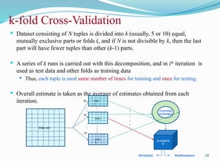
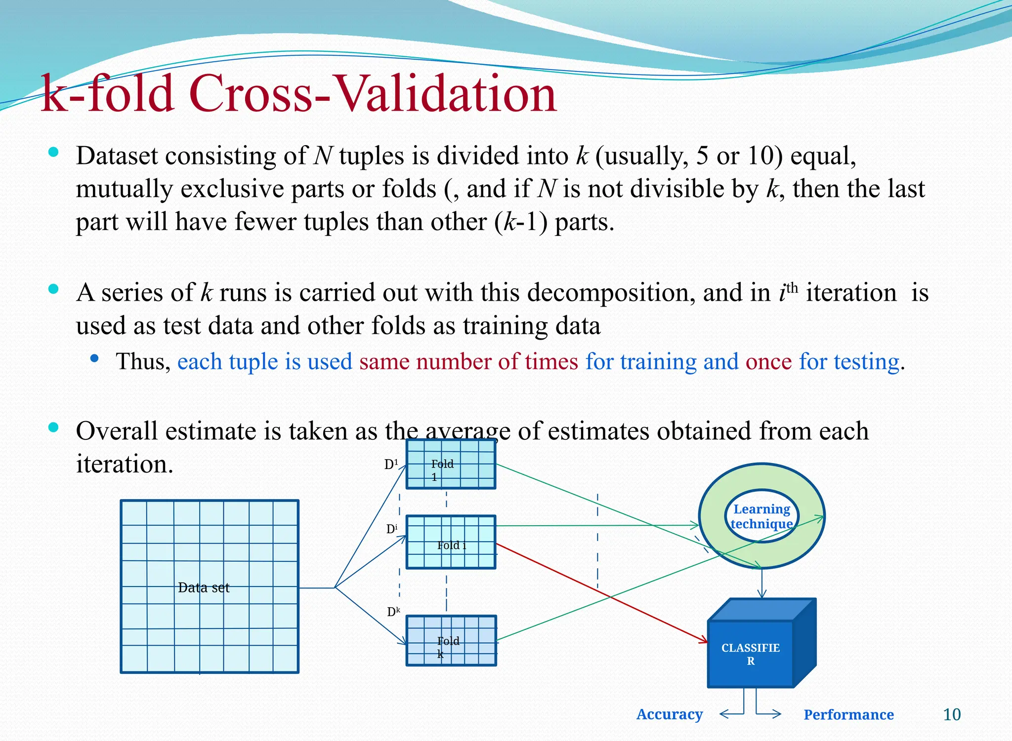
Datasetconsisting of N tuples is divided into k (usually, 5 or 10) equal,
mutually exclusive parts or folds (, and if N is not divisible by k, then the last
part will have fewer tuples than other (k-1) parts.
A series of k runs is carried out with this decomposition, and in ith
iteration is
used as test data and other folds as training data
Thus, each tuple is used same number of times for training and once for testing.
Overall estimate is taken as the average of estimates obtained from each
iteration.
10
Learning
technique
CLASSIFIE
R
D1
Di
Dk
Data set
Fold
1
Fold i
Fold
k
Accuracy Performance
11.
N-fold Cross-Validation
Ink-fold cross-validation method, part of the given data is used in training
with k-tests.
N-fold cross-validation is an extreme case of k-fold cross validation, often
known as “Leave-one-out’’ cross-validation.
Here, dataset is divided into as many folds as there are instances; thus, all
most each tuple forming a training set, building N classifiers.
In this method, therefore, N classifiers are built each with N-1 instances,
and one tuple is used to classify with a single test instance.
Test sets are mutually exclusive and effectively cover the entire set (in
sequence). This is as if trained by entire data as well as tested by entire data
set.
Overall estimation is then averaged out of the results of N classifiers.
11
12.
N-fold Cross-Validation :Issue
So far the estimation of accuracy and performance of a classifier model is
concerned, the N-fold cross-validation is comparable to the others we have
just discussed.
The drawback of N-fold cross validation strategy is that it is
computationally expensive, as here we have to repeat the run N times; this
is practically infeasible when data set is large.
In practice, the method is extremely beneficial with very small data set
only, where as much data as possible to need to be used to train a classifier.
12
13.
Bootstrap Method
TheBootstrap method is a variation of repeated version of Random
sampling method.
The method suggests the sampling of training records with replacement.
Each time a record is selected for training set, is put back into the original pool of
records, so that it is equally likely to be redrawn in the next run.
In other words, the Bootstrap method samples the given data set uniformly
with replacement.
The rational of having this strategy is that let some records be occur more
than once in the samples of both training as well as testing.
What is the probability that a record will be selected more than once?
13
14.
Bootstrap Method
Suppose,we have given a data set of N records. The data set is sampled N times
with replacement, resulting in a bootstrap sample (i.e., training set) of I samples.
Note that the entire runs are called a bootstrap sample in this method.
There are certain chance (i.e., probability) that a particular tuple occurs one or
more times in the training set
If they do not appear in the training set, then they will end up in the test set.
Each tuple has a probability of being selected (and the probability of not being
selected is .
We have to select N times, so the probability that a record will not be chosen during
the whole run is
Thus, the probability that a record is chosen by a bootstrap sample is
For a large value of N, it can be proved that
record chosen in a bootstrap sample is = 0.632
14
15.
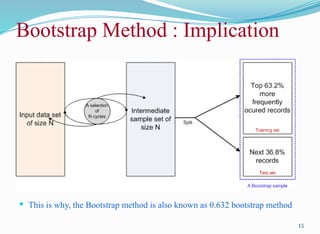
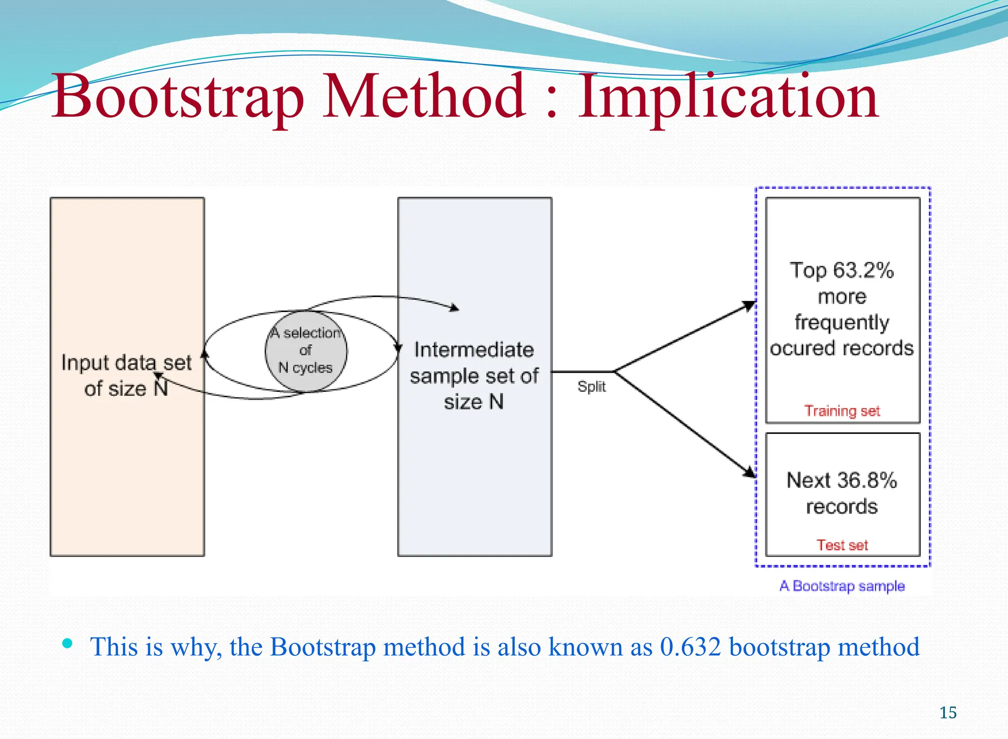
Bootstrap Method :Implication
15
This is why, the Bootstrap method is also known as 0.632 bootstrap method
Accuracy Estimation
Wehave learned how a classifier system can be tested. Next, we are to learn
the metrics with which a classifier should be estimated.
There are mainly to things to be measured for a given classifier
Accuracy
Performance
Accuracy estimation
If N is the number of instances with which a classifier is tested and p is the number
of correctly classified instances, the accuracy can be denoted as
Also, we can say the error rate (i.e., is misclassification rate) denoted by is denoted
by
17
18.
Accuracy : Trueand Predictive
Now, this accuracy may be true (or absolute) accuracy or predicted (or
optimistic) accuracy.
True accuracy of a classifier is the accuracy when the classifier is tested
with all possible unseen instances in the given classification space.
However, the number of possible unseen instances is potentially very large
(if it is not infinite)
For example, classifying a hand-written character
Hence, measuring the true accuracy beyond the dispute is impractical.
Predictive accuracy of a classifier is an accuracy estimation for a given
test data (which are mutually exclusive with training data).
If the predictive accuracy for test set is and if we test the classifier with a
different test set it is very likely that a different accuracy would be obtained.
The predictive accuracy when estimated with a given test set it should be
acceptable without any objection
18
19.
Predictive Accuracy
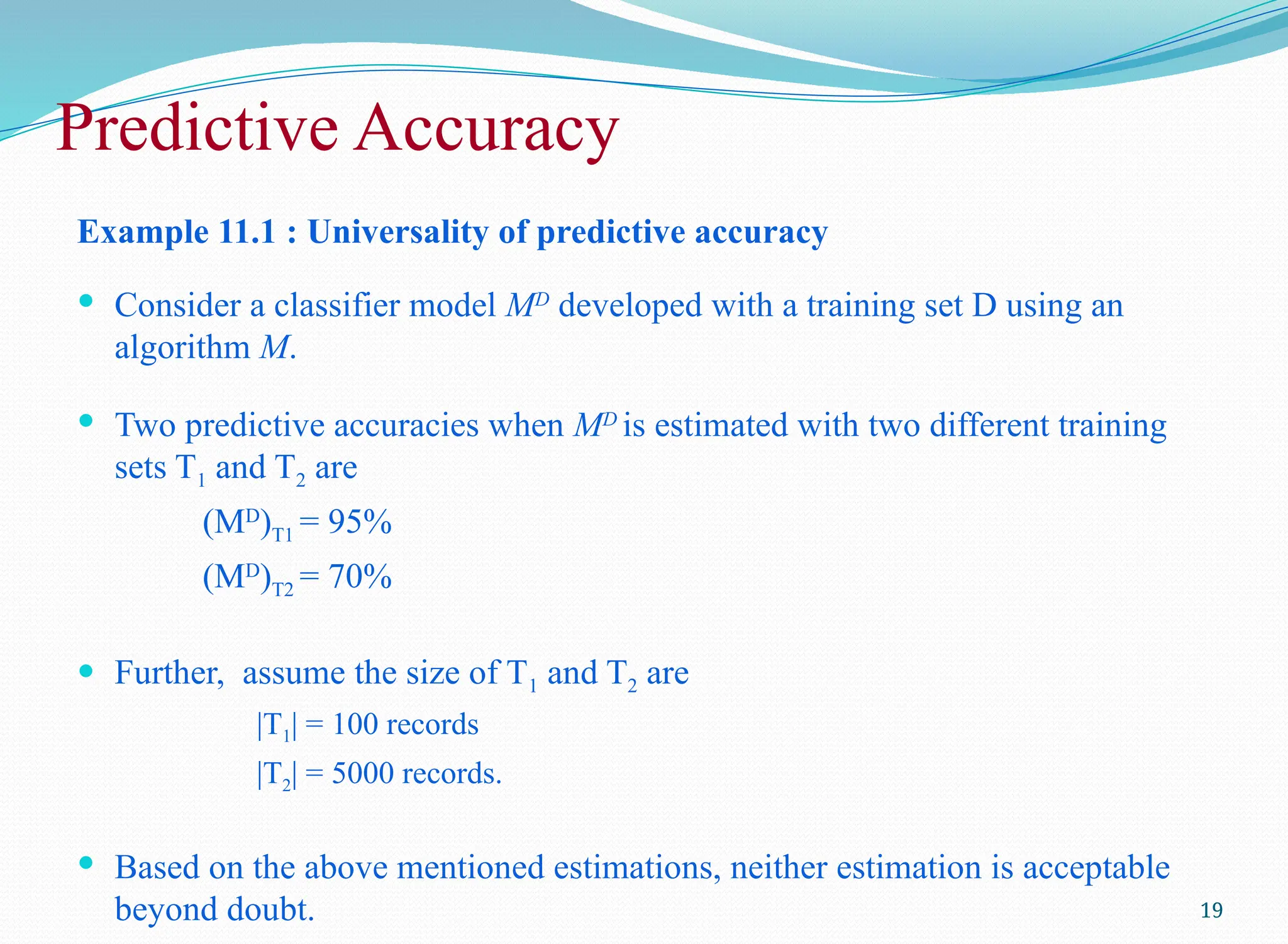
Example 11.1: Universality of predictive accuracy
Consider a classifier model MD
developed with a training set D using an
algorithm M.
Two predictive accuracies when MD
is estimated with two different training
sets T1 and T2 are
(MD
)T1 = 95%
(MD
)T2 = 70%
Further, assume the size of T1 and T2 are
|T1| = 100 records
|T2| = 5000 records.
Based on the above mentioned estimations, neither estimation is acceptable
beyond doubt. 19
20.
With theabove-mentioned issue in mind, researchers have proposed two
heuristic measures
Error estimation using Loss Functions
Statistical Estimation using Confidence Level
In the next few slides, we will discus about the two estimations
20
Predictive Accuracy
21.
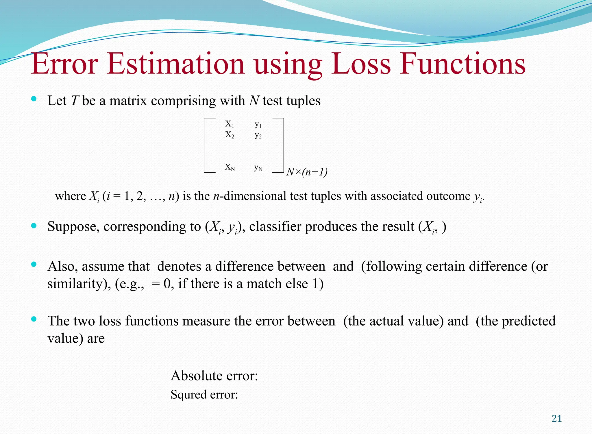
Let Tbe a matrix comprising with N test tuples
where Xi (i = 1, 2, …, n) is the n-dimensional test tuples with associated outcome yi.
Suppose, corresponding to (Xi, yi), classifier produces the result (Xi, )
Also, assume that denotes a difference between and (following certain difference (or
similarity), (e.g., = 0, if there is a match else 1)
The two loss functions measure the error between (the actual value) and (the predicted
value) are
Absolute error:
Squred error:
21
Error Estimation using Loss Functions
N×(n+1)
X1 y1
X2 y2
XN yN
22.
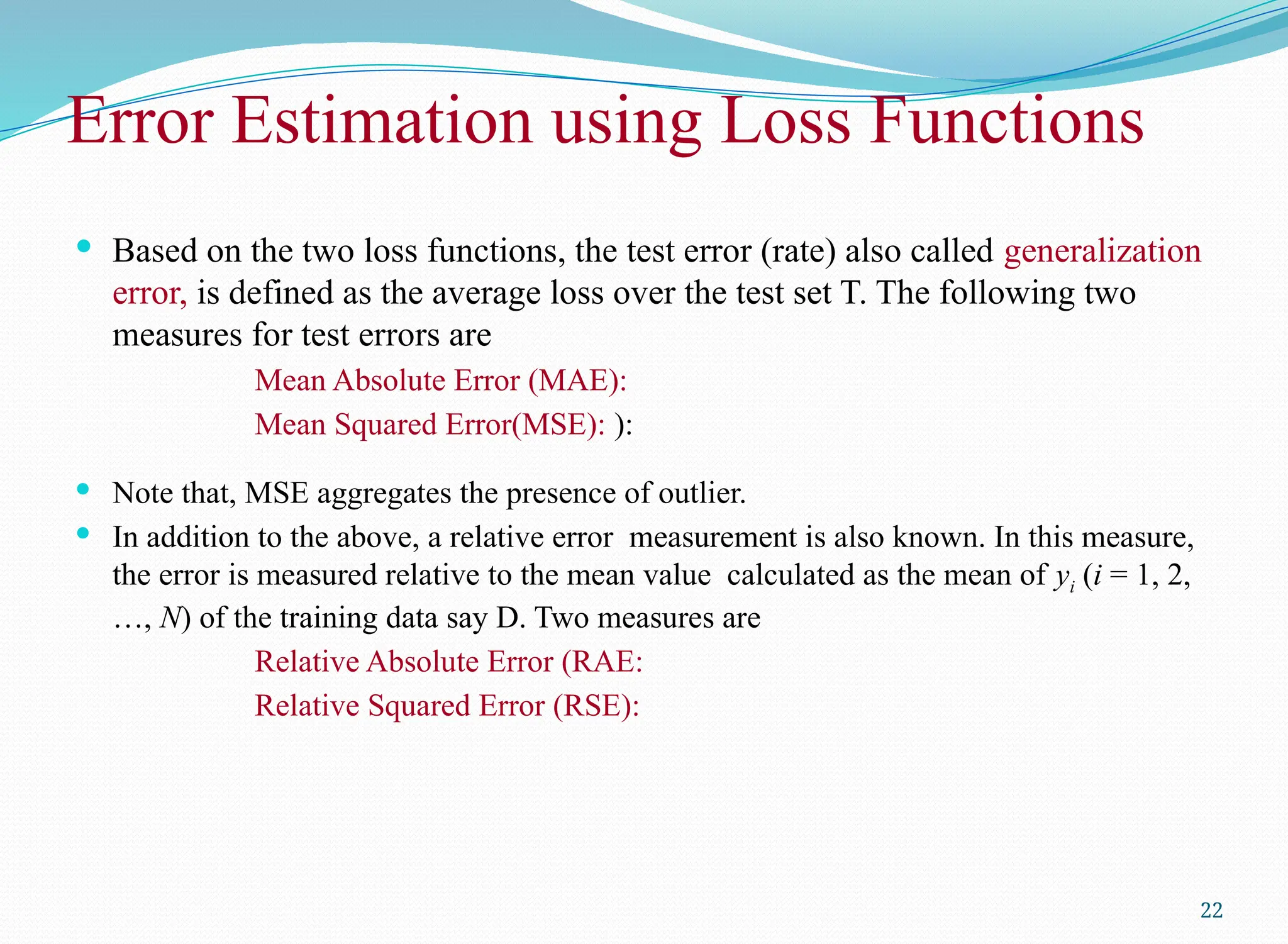
Based onthe two loss functions, the test error (rate) also called generalization
error, is defined as the average loss over the test set T. The following two
measures for test errors are
Mean Absolute Error (MAE):
Mean Squared Error(MSE): ):
Note that, MSE aggregates the presence of outlier.
In addition to the above, a relative error measurement is also known. In this measure,
the error is measured relative to the mean value calculated as the mean of yi (i = 1, 2,
…, N) of the training data say D. Two measures are
Relative Absolute Error (RAE:
Relative Squared Error (RSE):
22
Error Estimation using Loss Functions
23.
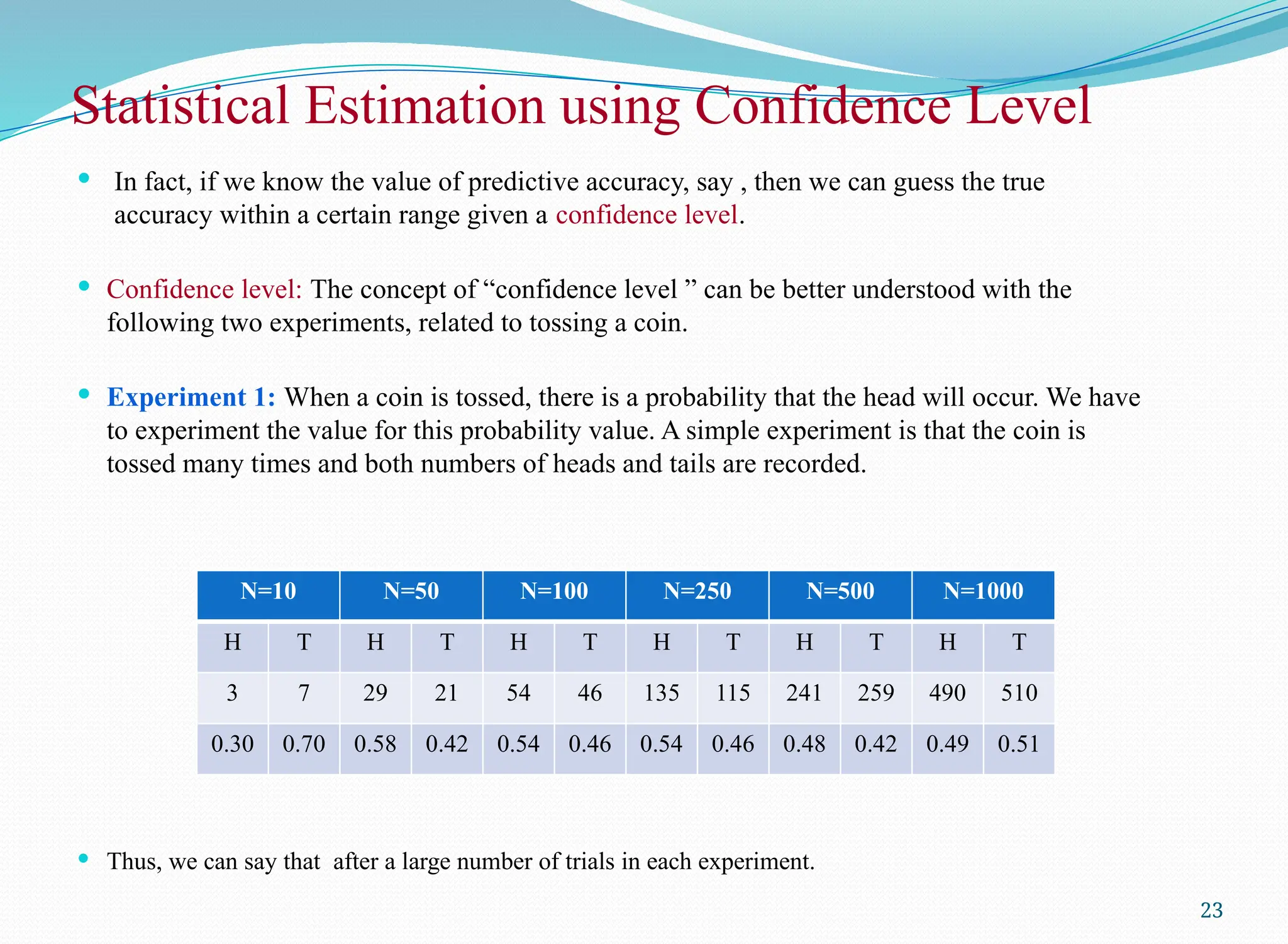
In fact,if we know the value of predictive accuracy, say , then we can guess the true
accuracy within a certain range given a confidence level.
Confidence level: The concept of “confidence level ” can be better understood with the
following two experiments, related to tossing a coin.
Experiment 1: When a coin is tossed, there is a probability that the head will occur. We have
to experiment the value for this probability value. A simple experiment is that the coin is
tossed many times and both numbers of heads and tails are recorded.
Thus, we can say that after a large number of trials in each experiment.
N=10 N=50 N=100 N=250 N=500 N=1000
H T H T H T H T H T H T
3 7 29 21 54 46 135 115 241 259 490 510
0.30 0.70 0.58 0.42 0.54 0.46 0.54 0.46 0.48 0.42 0.49 0.51
Statistical Estimation using Confidence Level
23
24.
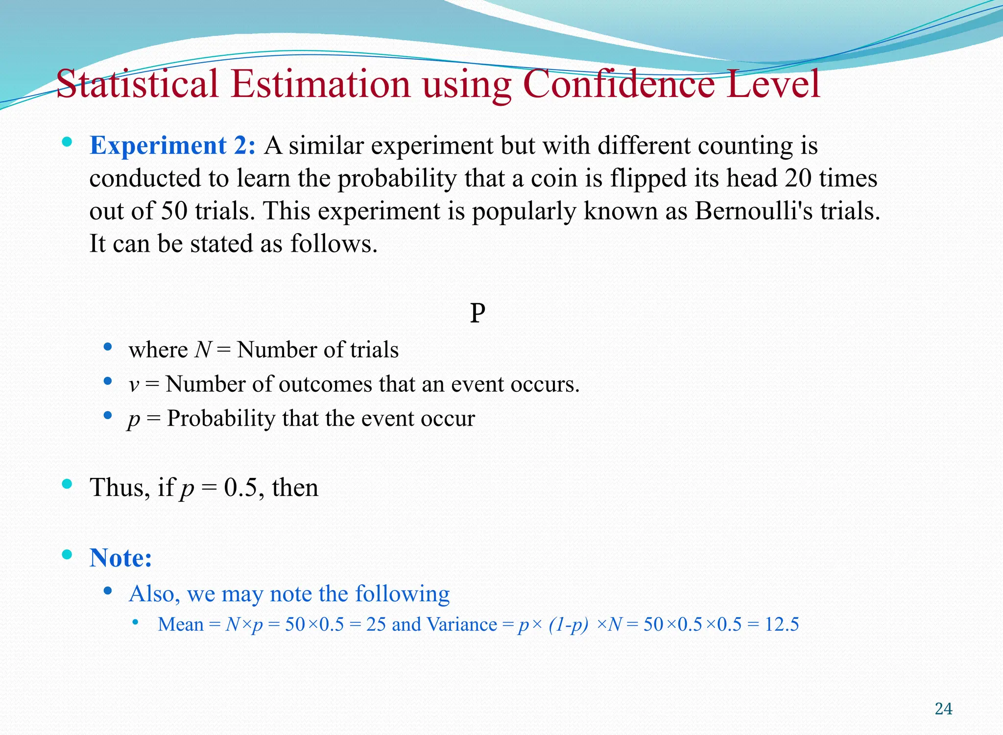
Experiment 2:A similar experiment but with different counting is
conducted to learn the probability that a coin is flipped its head 20 times
out of 50 trials. This experiment is popularly known as Bernoulli's trials.
It can be stated as follows.
P
where N = Number of trials
v = Number of outcomes that an event occurs.
p = Probability that the event occur
Thus, if p = 0.5, then
Note:
Also, we may note the following
Mean = N×p = 50×0.5 = 25 and Variance = p× (1-p) ×N = 50×0.5×0.5 = 12.5
Statistical Estimation using Confidence Level
24
25.
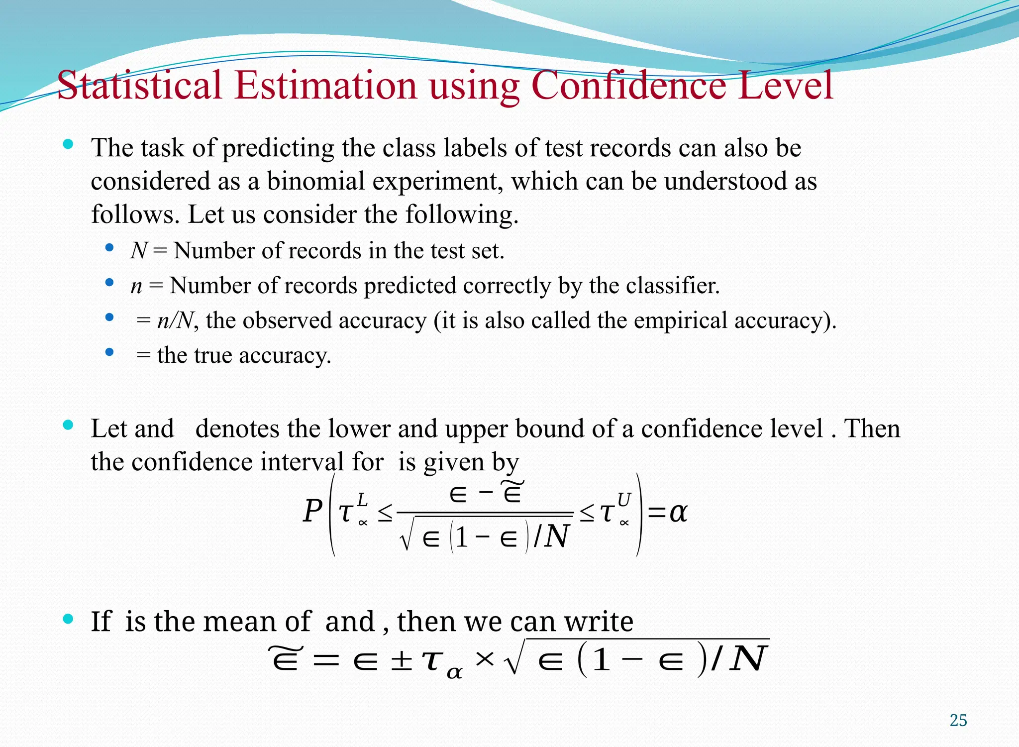
The taskof predicting the class labels of test records can also be
considered as a binomial experiment, which can be understood as
follows. Let us consider the following.
N = Number of records in the test set.
n = Number of records predicted correctly by the classifier.
= n/N, the observed accuracy (it is also called the empirical accuracy).
= the true accuracy.
Let and denotes the lower and upper bound of a confidence level . Then
the confidence interval for is given by
If is the mean of and , then we can write
Statistical Estimation using Confidence Level
25
𝑃
(𝜏∝
𝐿
≤
∈−~
∈
√∈(1−∈)/𝑁
≤𝜏∝
𝑈
)=𝛼
~
∈=∈± 𝜏𝛼 ×√∈(1 −∈)/ 𝑁
26.
A tableof with different values of can be obtained from any book on
statistics. A small part of the same is given below.
Thus, given a confidence level , we shall be able to know the value of and
hence the true accuracy (), if we have the value of the observed accuracy ().
Thus, knowing a test data set of size N, it is possible to estimate the true
accuracy!
Statistical Estimation using Confidence Level
26
0.5 0.7 0.8 0.9 0.95 0.98 0.99
0.67 1.04 1.28 1.65 1.96 2.33 2.58
~
∈=∈±𝝉𝜶 ×√∈(𝟏−∈)/𝑵
27.
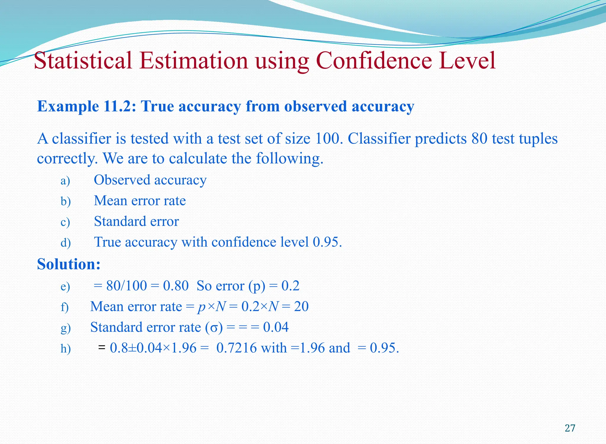
Example 11.2: Trueaccuracy from observed accuracy
A classifier is tested with a test set of size 100. Classifier predicts 80 test tuples
correctly. We are to calculate the following.
a) Observed accuracy
b) Mean error rate
c) Standard error
d) True accuracy with confidence level 0.95.
Solution:
e) = 80/100 = 0.80 So error (p) = 0.2
f) Mean error rate = p×N = 0.2×N = 20
g) Standard error rate (σ) = = = 0.04
h) = 0.8±0.04×1.96 = 0.7216 with =1.96 and = 0.95.
27
Statistical Estimation using Confidence Level
28.
Note:
Suppose, aclassifier is tested k times with k different test sets. If i denotes the
predicted accuracy when tested with test set Ni in the i-th run (1≤ i ≤ k), then
the overall predicted accuracy is
Thus, is the weighted average of values. The standard error and true accuracy
at a confidence are
28
Statistical Estimation using Confidence Level
Performance Estimation ofa Classifier
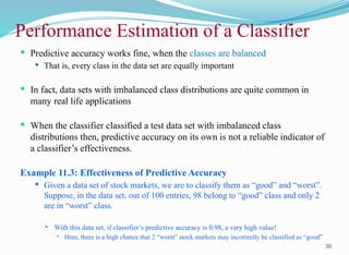
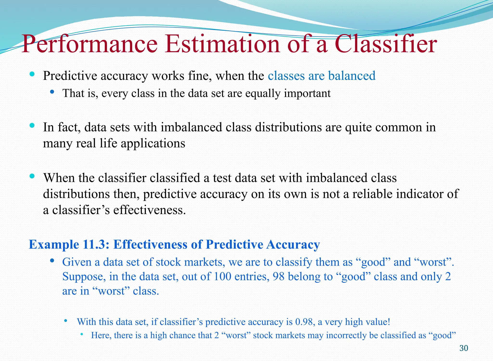
Predictive accuracy works fine, when the classes are balanced
That is, every class in the data set are equally important
In fact, data sets with imbalanced class distributions are quite common in
many real life applications
When the classifier classified a test data set with imbalanced class
distributions then, predictive accuracy on its own is not a reliable indicator of
a classifier’s effectiveness.
Example 11.3: Effectiveness of Predictive Accuracy
Given a data set of stock markets, we are to classify them as “good” and “worst”.
Suppose, in the data set, out of 100 entries, 98 belong to “good” class and only 2
are in “worst” class.
With this data set, if classifier’s predictive accuracy is 0.98, a very high value!
Here, there is a high chance that 2 “worst” stock markets may incorrectly be classified as “good”
30
31.
Performance Estimation ofa Classifier
Thus, when the classifier classified a test data set with imbalanced class
distributions, then predictive accuracy on its own is not a reliable indicator of
a classifier’s effectiveness.
This necessitates an alternative metrics to judge the classifier.
Before exploring them, we introduce the concept of Confusion matrix.
31
32.
Confusion Matrix
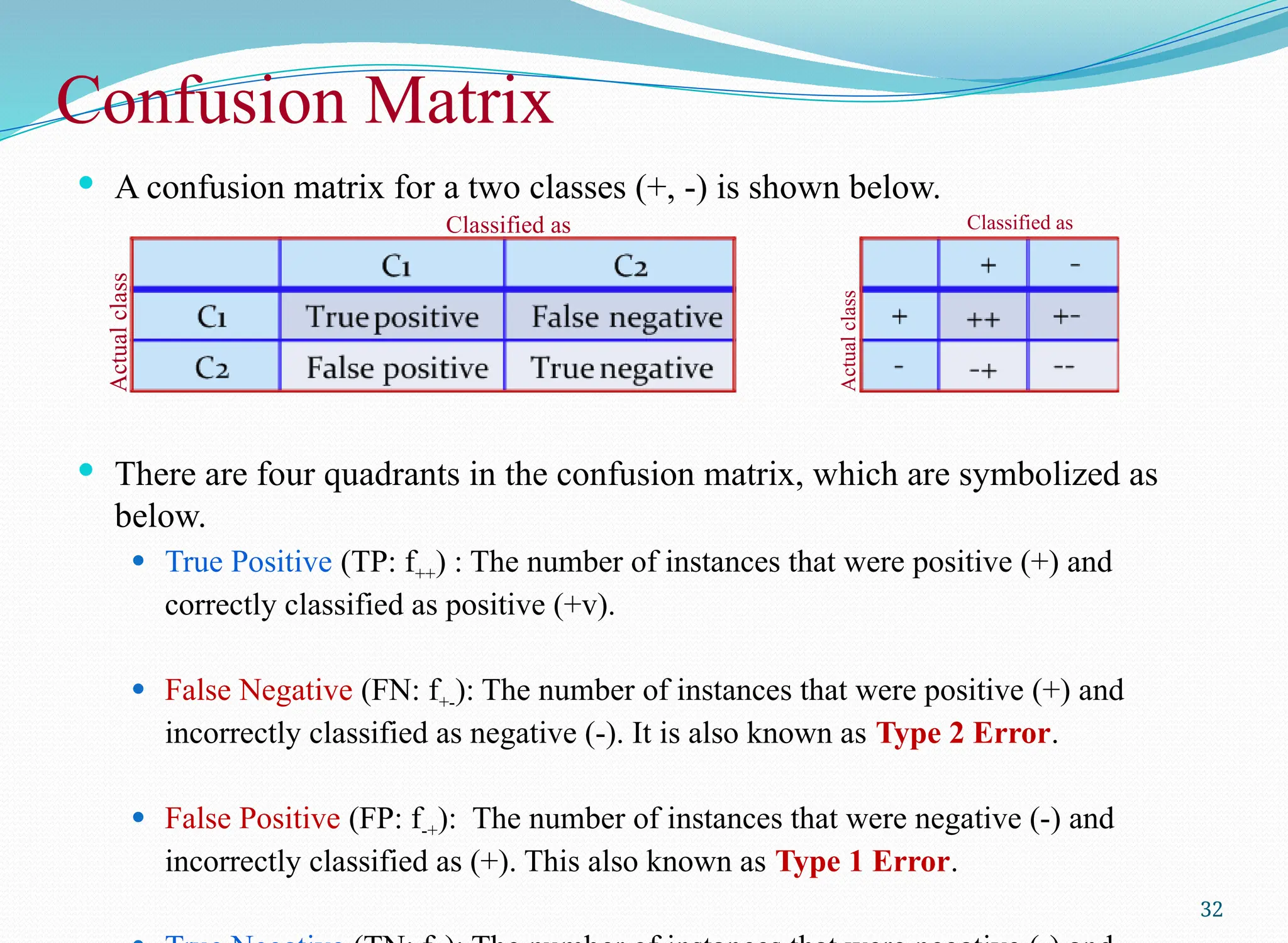
Aconfusion matrix for a two classes (+, -) is shown below.
There are four quadrants in the confusion matrix, which are symbolized as
below.
True Positive (TP: f++) : The number of instances that were positive (+) and
correctly classified as positive (+v).
False Negative (FN: f+-): The number of instances that were positive (+) and
incorrectly classified as negative (-). It is also known as Type 2 Error.
False Positive (FP: f-+): The number of instances that were negative (-) and
incorrectly classified as (+). This also known as Type 1 Error.
32
Classified as
Actual
class
Classified as
Actual
class
33.
Confusion Matrix: SummaryInformation
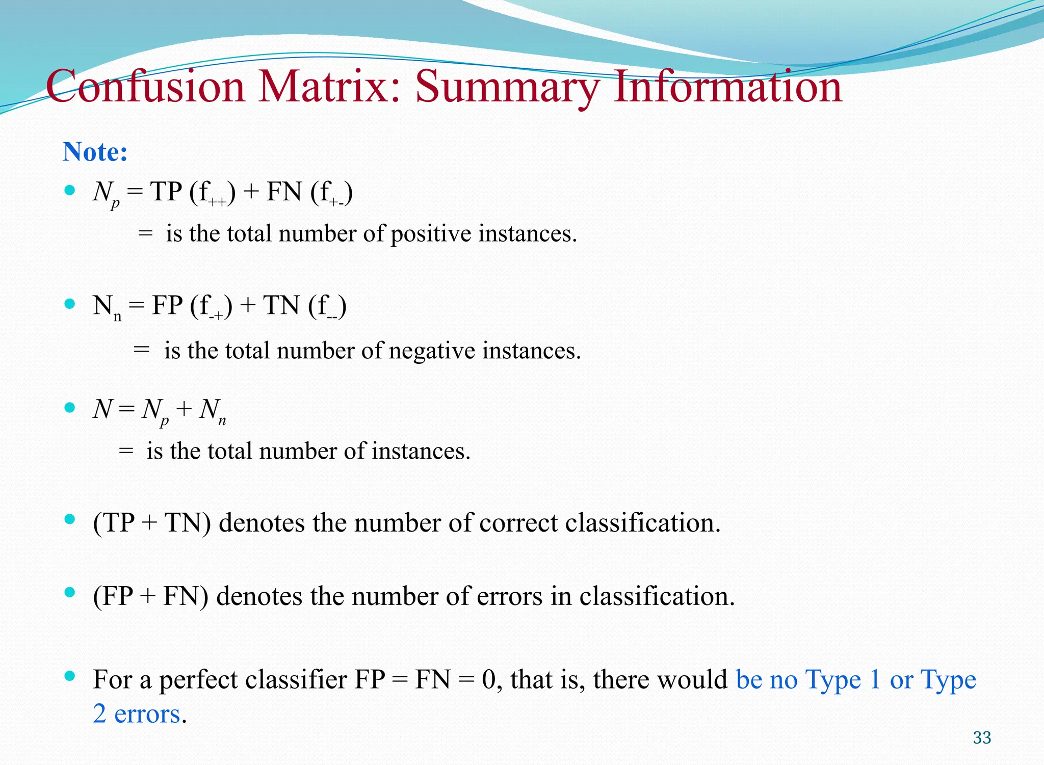
Note:
Np = TP (f++) + FN (f+-)
= is the total number of positive instances.
Nn = FP (f-+) + TN (f--)
= is the total number of negative instances.
N = Np + Nn
= is the total number of instances.
(TP + TN) denotes the number of correct classification.
(FP + FN) denotes the number of errors in classification.
For a perfect classifier FP = FN = 0, that is, there would be no Type 1 or Type
2 errors.
33
34.
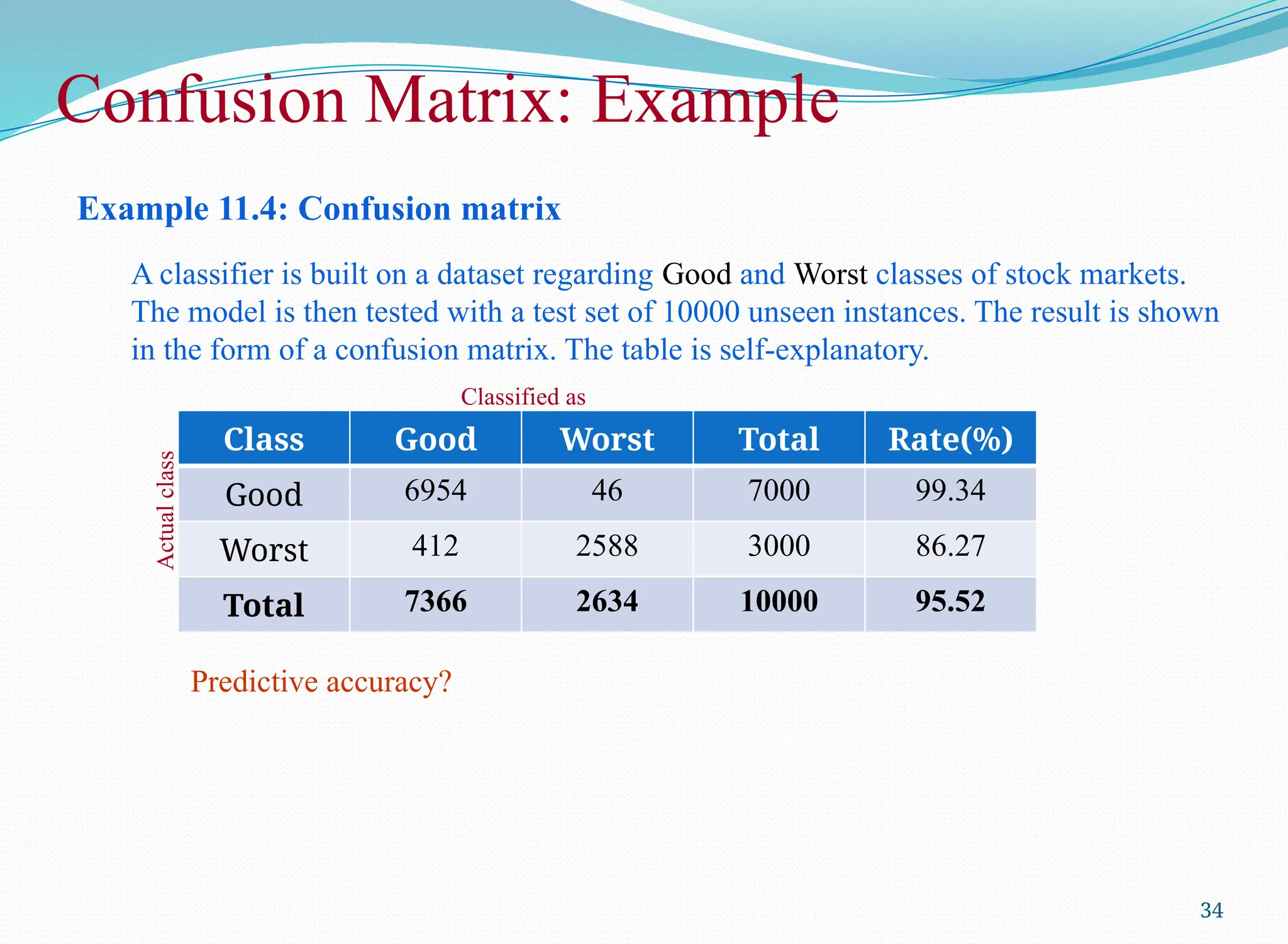
Example 11.4: Confusionmatrix
A classifier is built on a dataset regarding Good and Worst classes of stock markets.
The model is then tested with a test set of 10000 unseen instances. The result is shown
in the form of a confusion matrix. The table is self-explanatory.
34
Class Good Worst Total Rate(%)
Good 6954 46 7000 99.34
Worst 412 2588 3000 86.27
Total 7366 2634 10000 95.52
Confusion Matrix: Example
Predictive accuracy?
Classified as
Actual
class
35.
Confusion Matrix forMulticlass Classifier
Having m classes, confusion matrix is a table of size m×m , where,
element at (i, j) indicates the number of instances of class i but
classified as class j.
To have good accuracy for a classifier, ideally most diagonal entries
should have large values with the rest of entries being close to zero.
Note:
Confusion matrix may have additional rows or columns to provide total
or recognition rates per class.
35
36.
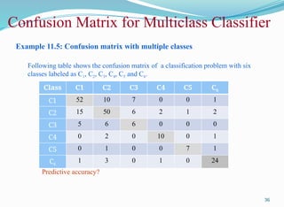
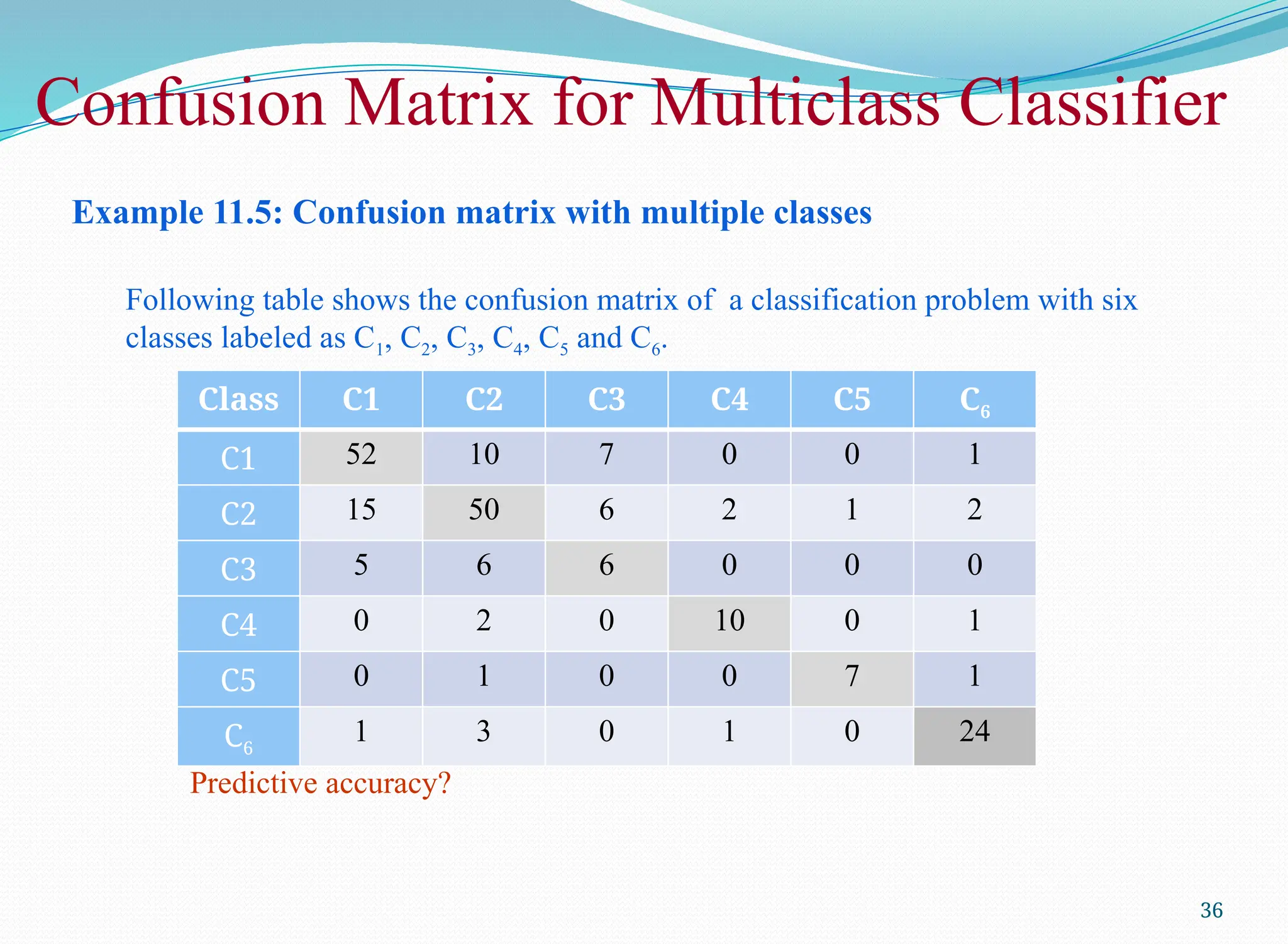
Example 11.5: Confusionmatrix with multiple classes
Following table shows the confusion matrix of a classification problem with six
classes labeled as C1, C2, C3, C4, C5 and C6.
36
Class C1 C2 C3 C4 C5 C6
C1 52 10 7 0 0 1
C2 15 50 6 2 1 2
C3 5 6 6 0 0 0
C4 0 2 0 10 0 1
C5 0 1 0 0 7 1
C6
1 3 0 1 0 24
Confusion Matrix for Multiclass Classifier
Predictive accuracy?
37.
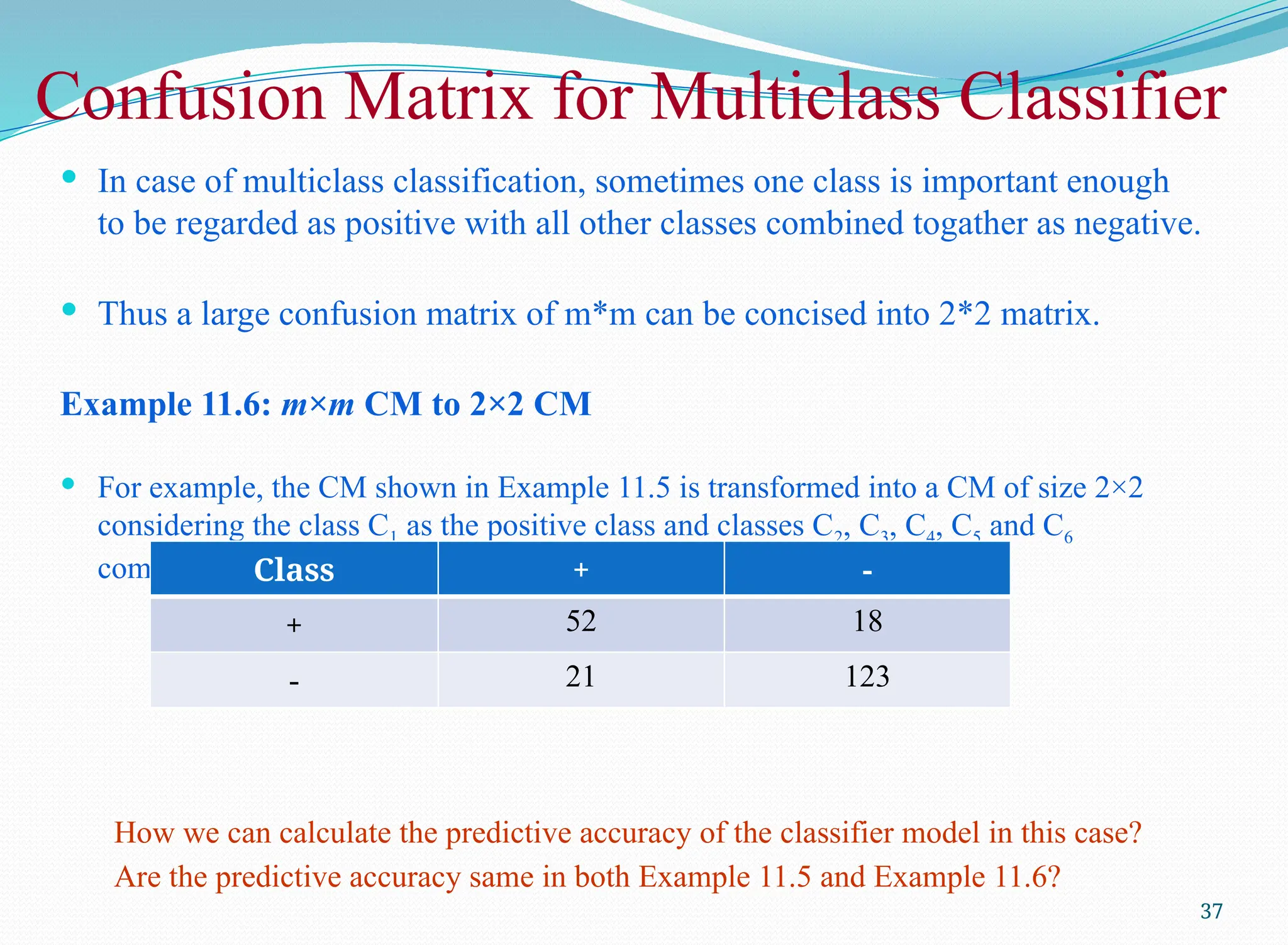
In caseof multiclass classification, sometimes one class is important enough
to be regarded as positive with all other classes combined togather as negative.
Thus a large confusion matrix of m*m can be concised into 2*2 matrix.
Example 11.6: m×m CM to 2×2 CM
For example, the CM shown in Example 11.5 is transformed into a CM of size 2×2
considering the class C1 as the positive class and classes C2, C3, C4, C5 and C6
combined together as negative.
How we can calculate the predictive accuracy of the classifier model in this case?
Are the predictive accuracy same in both Example 11.5 and Example 11.6?
37
Class + -
+ 52 18
- 21 123
Confusion Matrix for Multiclass Classifier
38.
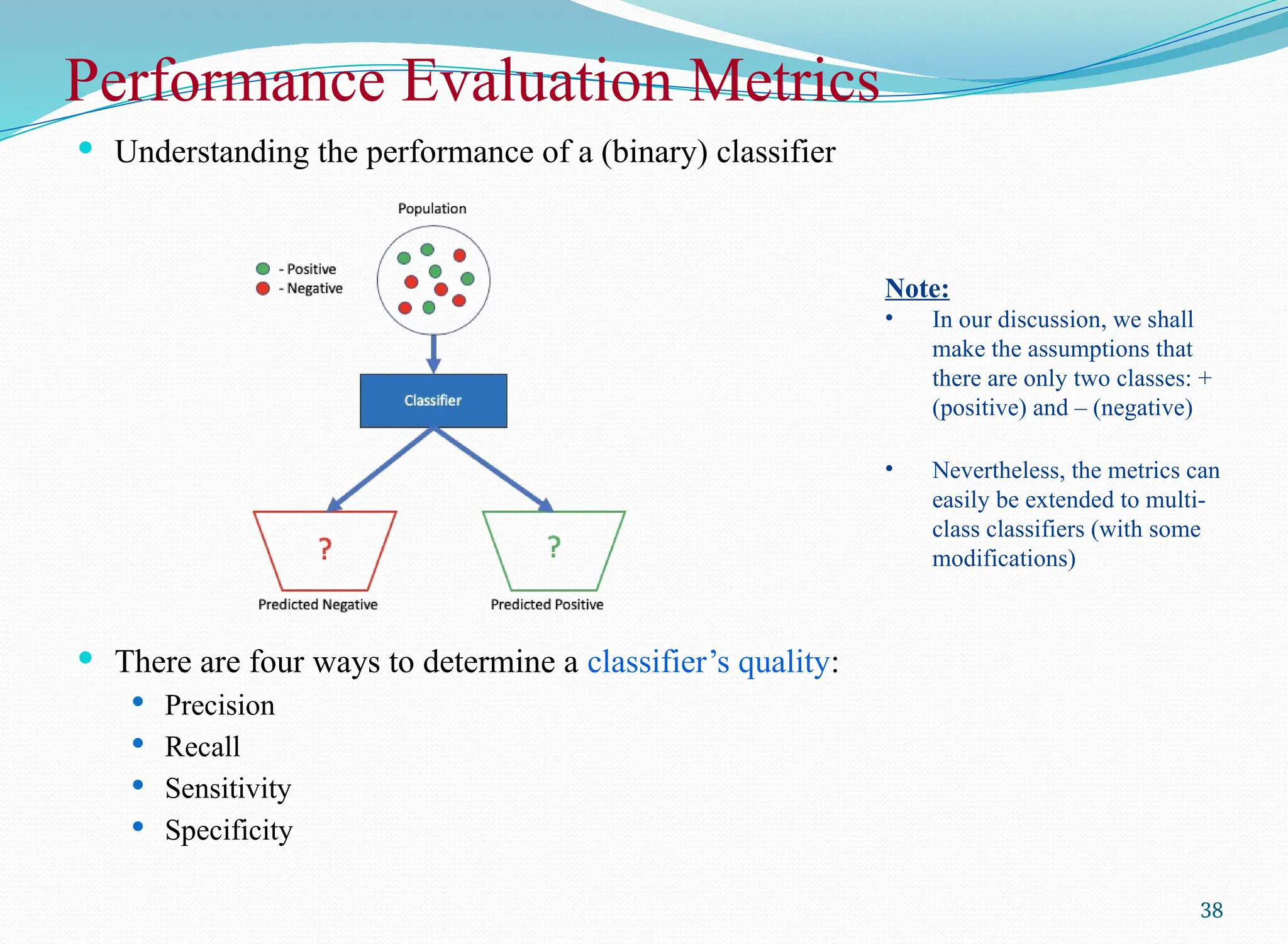
Performance Evaluation Metrics
Understanding the performance of a (binary) classifier
There are four ways to determine a classifier’s quality:
Precision
Recall
Sensitivity
Specificity
38
Note:
• In our discussion, we shall
make the assumptions that
there are only two classes: +
(positive) and – (negative)
• Nevertheless, the metrics can
easily be extended to multi-
class classifiers (with some
modifications)
39.
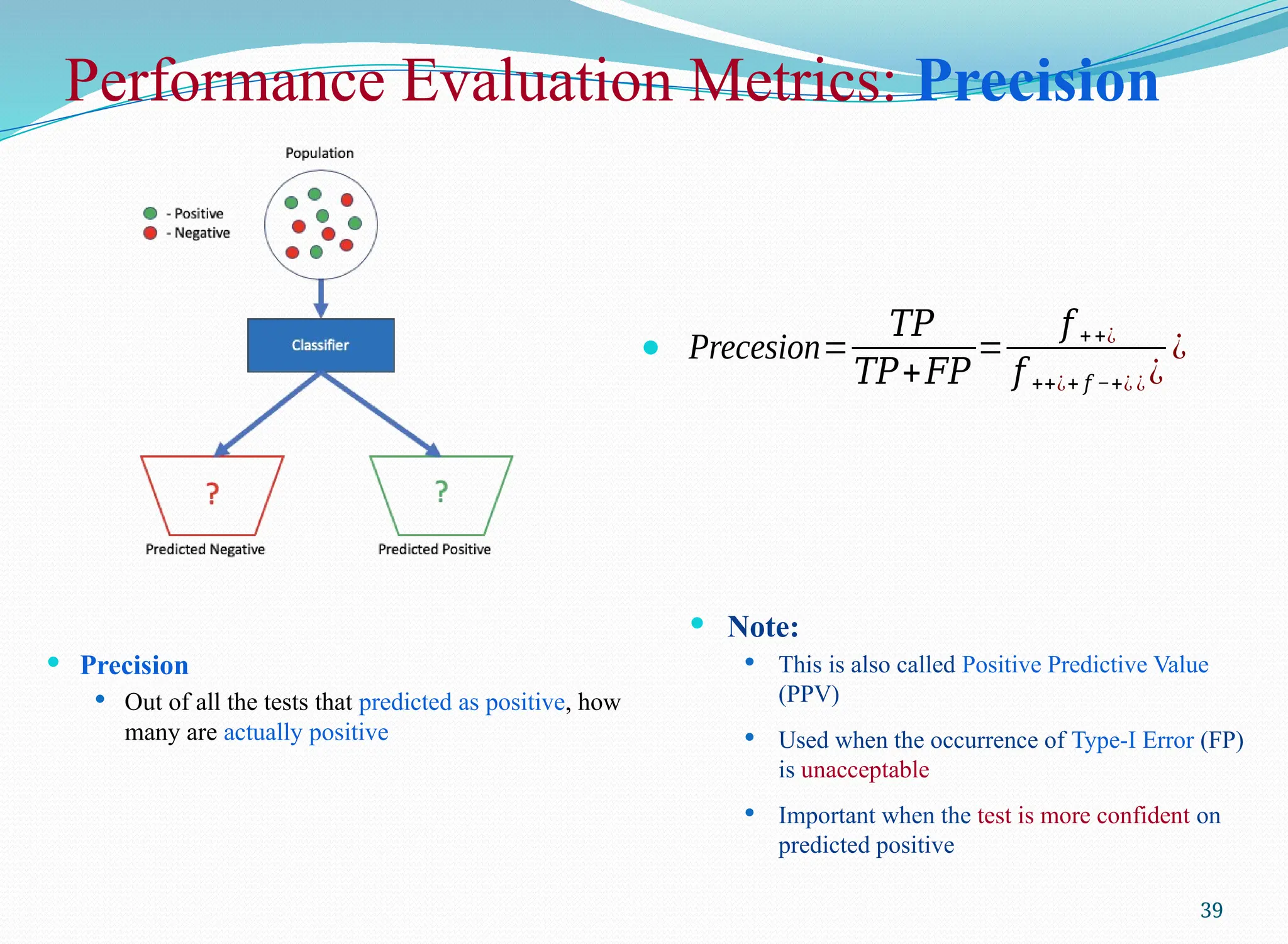
Performance Evaluation Metrics:Precision
Precision
Out of all the tests that predicted as positive, how
many are actually positive
39
Precesion=
𝑇𝑃
𝑇𝑃+𝐹𝑃
=
𝑓 ++¿
𝑓 ++¿+ 𝑓 −+¿ ¿ ¿
¿
Note:
This is also called Positive Predictive Value
(PPV)
Used when the occurrence of Type-I Error (FP)
is unacceptable
Important when the test is more confident on
predicted positive
40.
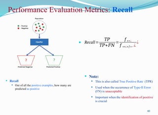
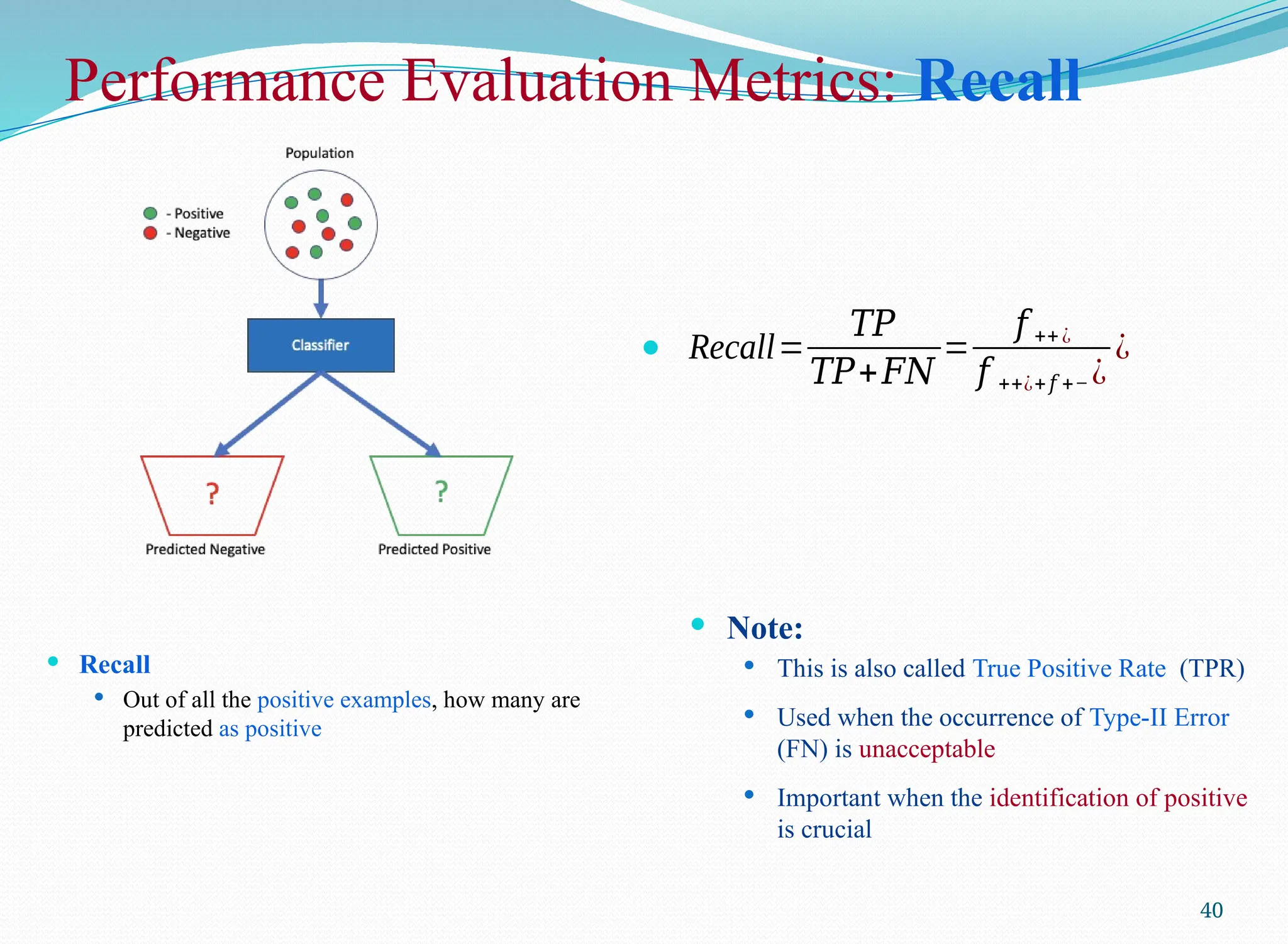
Performance Evaluation Metrics:Recall
Recall
Out of all the positive examples, how many are
predicted as positive
40
Recall=
𝑇𝑃
𝑇𝑃+𝐹𝑁
=
𝑓 ++¿
𝑓 ++¿+𝑓 +− ¿
¿
Note:
This is also called True Positive Rate (TPR)
Used when the occurrence of Type-II Error
(FN) is unacceptable
Important when the identification of positive
is crucial
41.
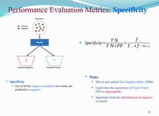
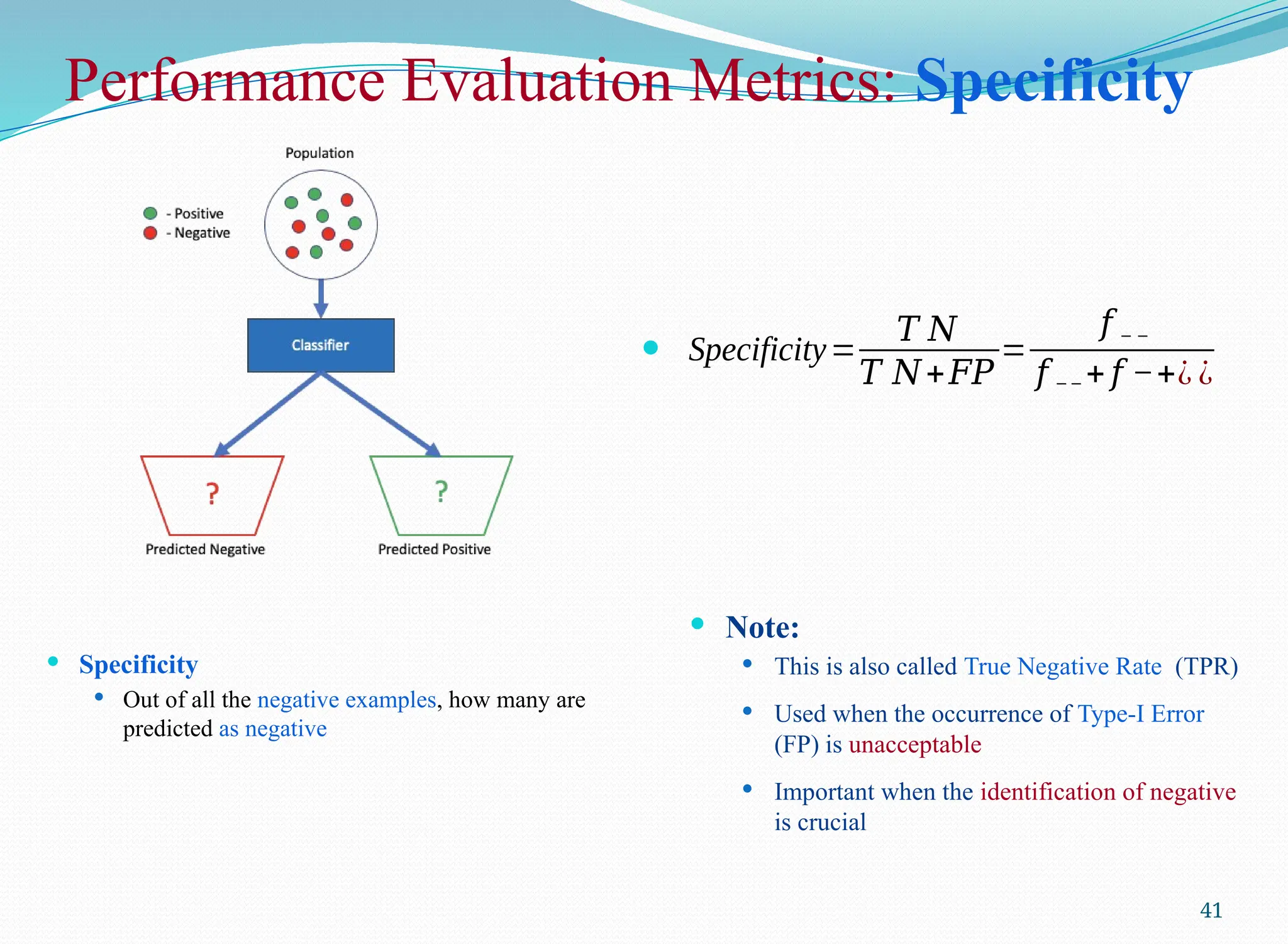
Performance Evaluation Metrics:Specificity
Specificity
Out of all the negative examples, how many are
predicted as negative
41
Specificity=
𝑇 𝑁
𝑇 𝑁+𝐹𝑃
=
𝑓 − −
𝑓 −− + 𝑓 −+¿ ¿
Note:
This is also called True Negative Rate (TPR)
Used when the occurrence of Type-I Error
(FP) is unacceptable
Important when the identification of negative
is crucial
42.
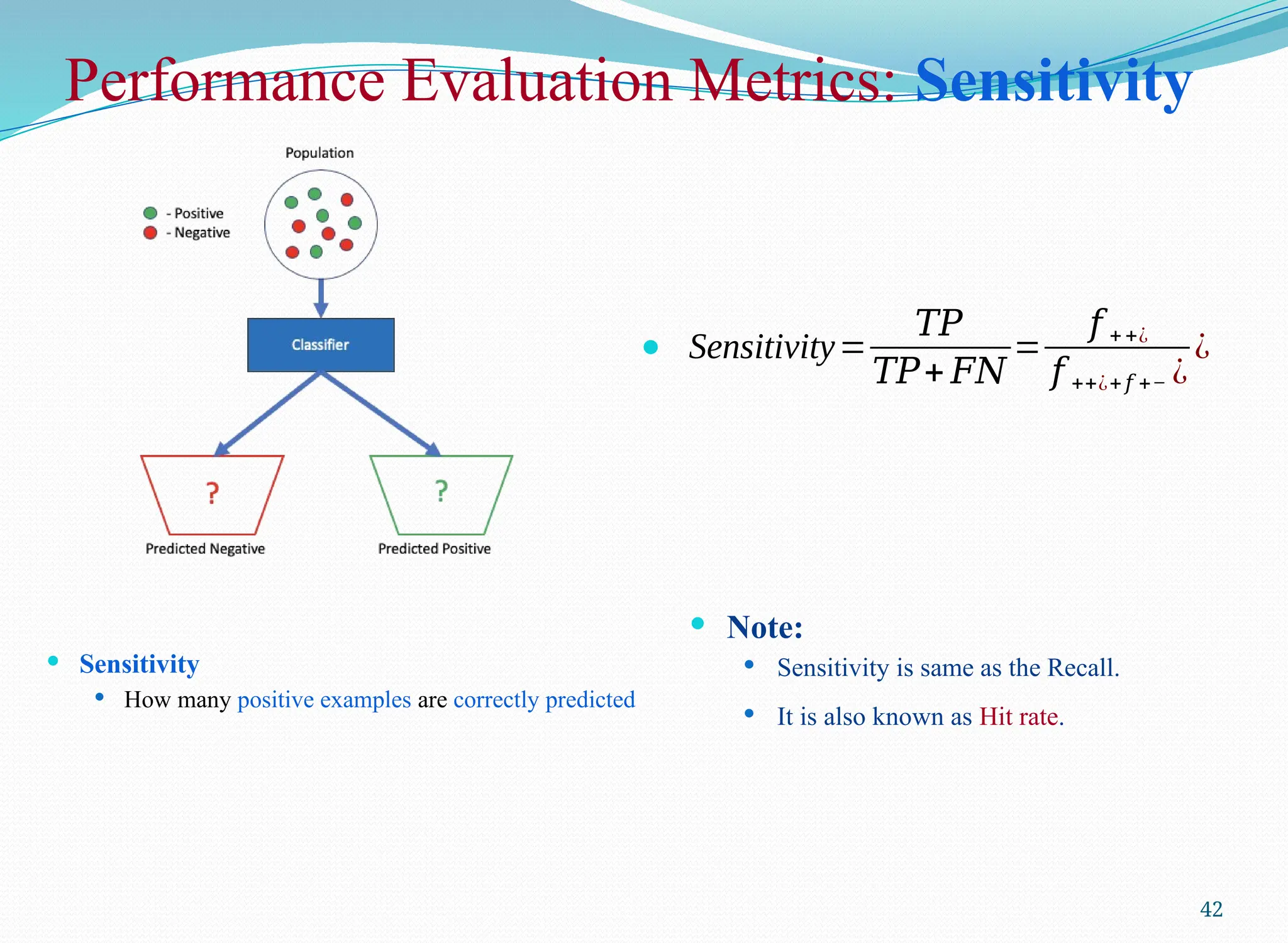
Performance Evaluation Metrics:Sensitivity
Sensitivity
How many positive examples are correctly predicted
42
Sensitivity=
𝑇𝑃
𝑇𝑃+ 𝐹𝑁
=
𝑓 ++¿
𝑓 ++¿+𝑓 +− ¿
¿
Note:
Sensitivity is same as the Recall.
It is also known as Hit rate.
43.
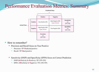
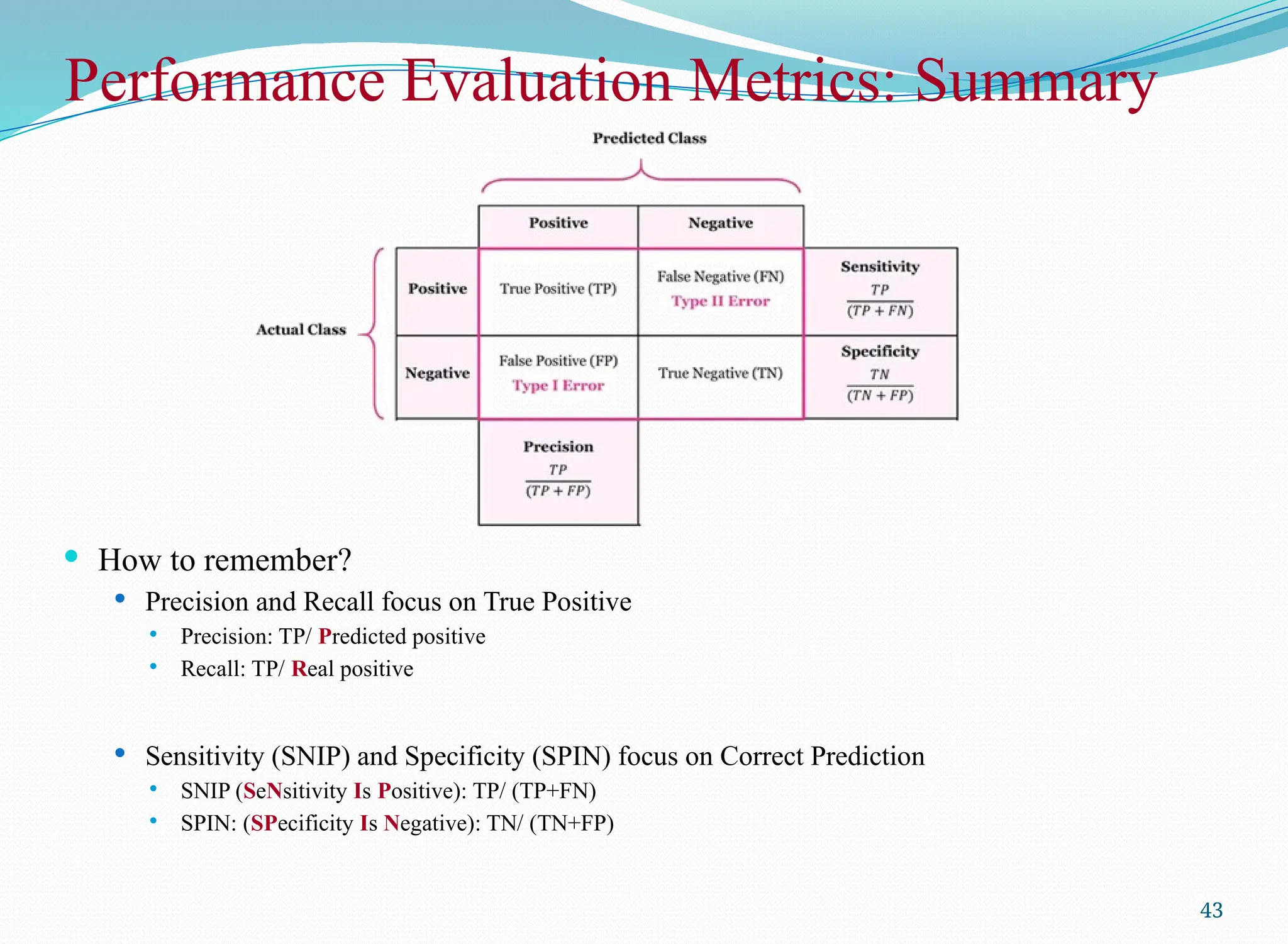
Performance Evaluation Metrics:Summary
How to remember?
Precision and Recall focus on True Positive
Precision: TP/ Predicted positive
Recall: TP/ Real positive
Sensitivity (SNIP) and Specificity (SPIN) focus on Correct Prediction
SNIP (SeNsitivity Is Positive): TP/ (TP+FN)
SPIN: (SPecificity Is Negative): TN/ (TN+FP)
43
44.
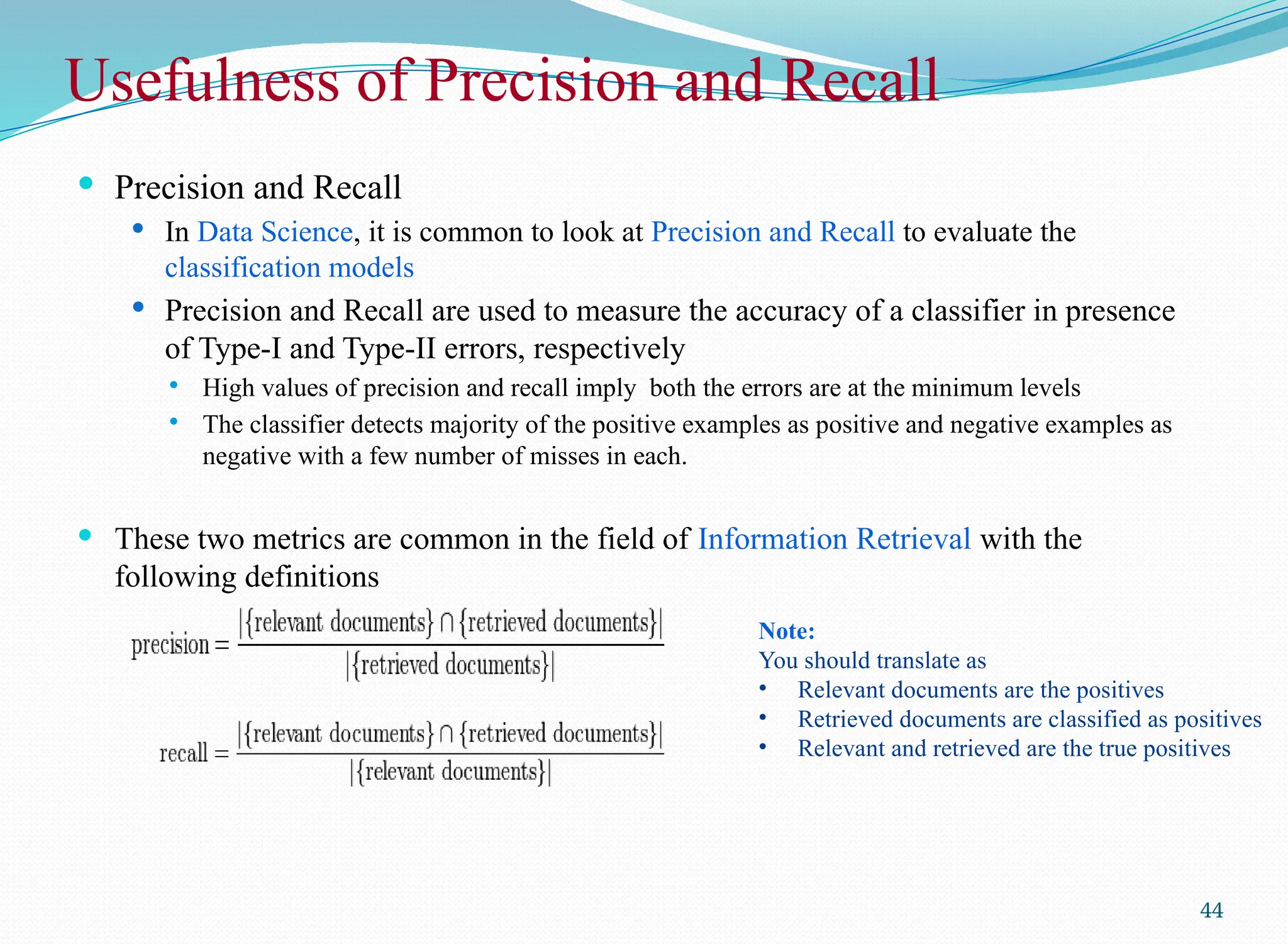
Usefulness of Precisionand Recall
Precision and Recall
In Data Science, it is common to look at Precision and Recall to evaluate the
classification models
Precision and Recall are used to measure the accuracy of a classifier in presence
of Type-I and Type-II errors, respectively
High values of precision and recall imply both the errors are at the minimum levels
The classifier detects majority of the positive examples as positive and negative examples as
negative with a few number of misses in each.
These two metrics are common in the field of Information Retrieval with the
following definitions
44
Note:
You should translate as
• Relevant documents are the positives
• Retrieved documents are classified as positives
• Relevant and retrieved are the true positives
45.
45
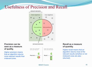
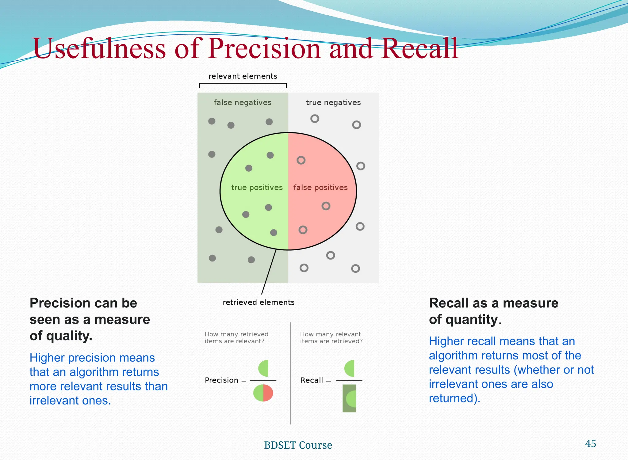
Usefulness of Precisionand Recall
BDSET Course
Precision can be
seen as a measure
of quality.
Recall as a measure
of quantity.
Higher precision means
that an algorithm returns
more relevant results than
irrelevant ones.
Higher recall means that an
algorithm returns most of the
relevant results (whether or not
irrelevant ones are also
returned).
46.
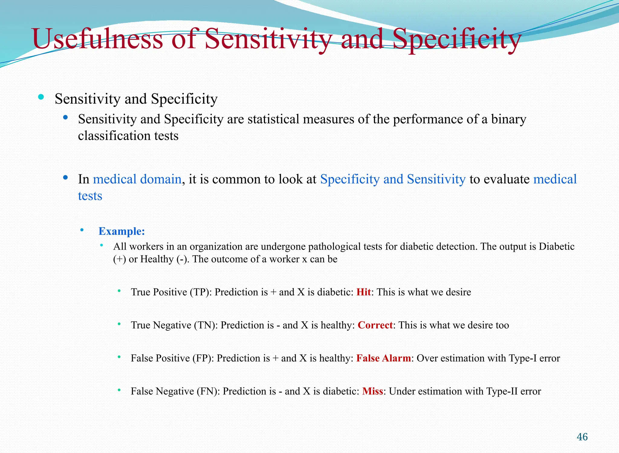
Usefulness of Sensitivityand Specificity
Sensitivity and Specificity
Sensitivity and Specificity are statistical measures of the performance of a binary
classification tests
In medical domain, it is common to look at Specificity and Sensitivity to evaluate medical
tests
Example:
All workers in an organization are undergone pathological tests for diabetic detection. The output is Diabetic
(+) or Healthy (-). The outcome of a worker x can be
True Positive (TP): Prediction is + and X is diabetic: Hit: This is what we desire
True Negative (TN): Prediction is - and X is healthy: Correct: This is what we desire too
False Positive (FP): Prediction is + and X is healthy: False Alarm: Over estimation with Type-I error
False Negative (FN): Prediction is - and X is diabetic: Miss: Under estimation with Type-II error
46
47.
47
Sensitivity and Specificity
BDSETCourse
Sensitivity refers to a test's
ability to designate an
individual with disease as
positive.
A highly sensitive test means
that there are few false
negative results, and thus
fewer cases of disease are
missed.
Specificity refers to a test's
ability to designate an
individual who does not
have a disease as negative.
A high specificity test means
that there less miss
classification.
48.
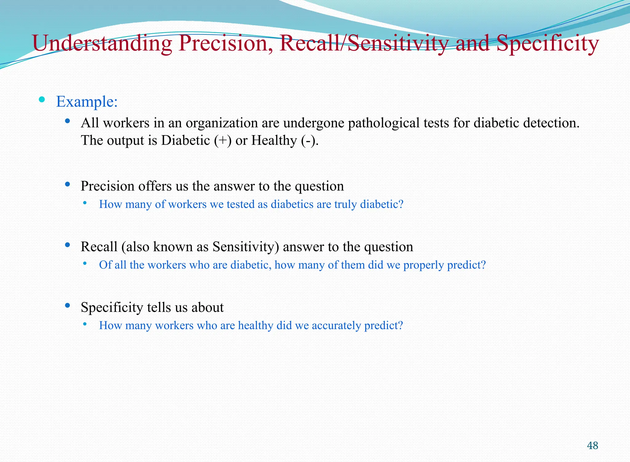
Understanding Precision, Recall/Sensitivityand Specificity
Example:
All workers in an organization are undergone pathological tests for diabetic detection.
The output is Diabetic (+) or Healthy (-).
Precision offers us the answer to the question
How many of workers we tested as diabetics are truly diabetic?
Recall (also known as Sensitivity) answer to the question
Of all the workers who are diabetic, how many of them did we properly predict?
Specificity tells us about
How many workers who are healthy did we accurately predict?
48
49.
Performance Evaluation Metrics
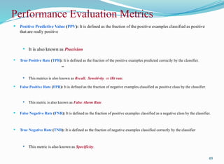
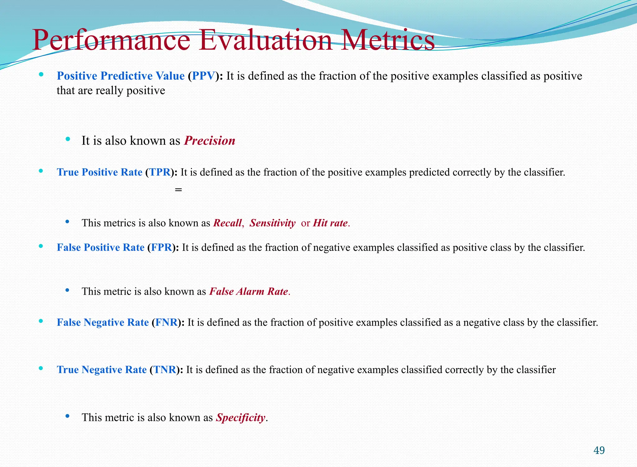
Positive Predictive Value (PPV): It is defined as the fraction of the positive examples classified as positive
that are really positive
It is also known as Precision
True Positive Rate (TPR): It is defined as the fraction of the positive examples predicted correctly by the classifier.
=
This metrics is also known as Recall, Sensitivity or Hit rate.
False Positive Rate (FPR): It is defined as the fraction of negative examples classified as positive class by the classifier.
This metric is also known as False Alarm Rate.
False Negative Rate (FNR): It is defined as the fraction of positive examples classified as a negative class by the classifier.
True Negative Rate (TNR): It is defined as the fraction of negative examples classified correctly by the classifier
This metric is also known as Specificity.
49
50.
50
F1 Score(F1): Recall (r) and Precision (p) are two widely used metrics employed in
analysis, where detection of one of the classes is considered more significant than the others.
It is defined in terms of (r or TPR) and (p or PPV) as follows.
Note
F1 represents the harmonic mean between recall and precision
High value of F1 score ensures that both Precision and Recall are reasonably high.
Performance Evaluation Metrics: F1 Score
51.
51
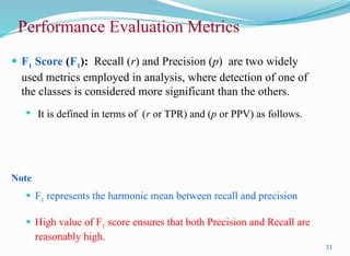
F1 Score(F1): Recall (r) and Precision (p) are two widely
used metrics employed in analysis, where detection of one of
the classes is considered more significant than the others.
It is defined in terms of (r or TPR) and (p or PPV) as follows.
Note
F1 represents the harmonic mean between recall and precision
High value of F1 score ensures that both Precision and Recall are
reasonably high.
Performance Evaluation Metrics
52.
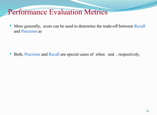
More generally,score can be used to determine the trade-off between Recall
and Precision as
Both, Precision and Recall are special cases of when and , respectively.
52
Performance Evaluation Metrics
53.
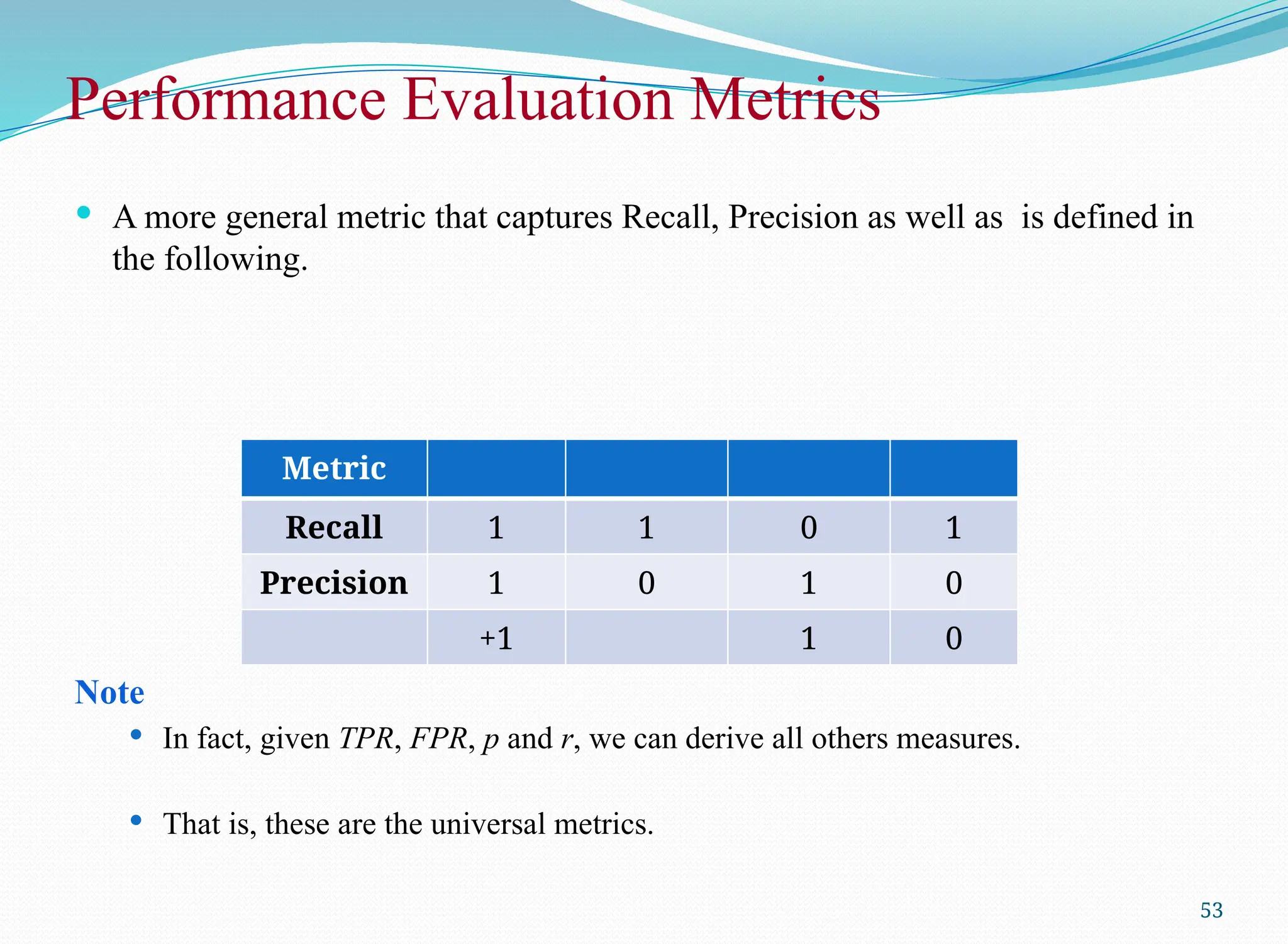
A moregeneral metric that captures Recall, Precision as well as is defined in
the following.
Note
In fact, given TPR, FPR, p and r, we can derive all others measures.
That is, these are the universal metrics.
53
Metric
Recall 1 1 0 1
Precision 1 0 1 0
+1 1 0
Performance Evaluation Metrics
54.
Predictive Accuracy (ε)
It is defined as the fraction of the number of examples that are correctly
classified by the classifier to the total number of instances.
This accuracy is equivalent to Fw with w1= w2= w3= w4=1.
54
55.
Error Rate ()
The error rate is defined as the fraction of the examples that are
incorrectly classified.
Note
.
55
56.
Predictive accuracy() can be expressed in terms of sensitivity and specificity.
We can write
Thus,
56
Accuracy, Sensitivity and Specificity
57.
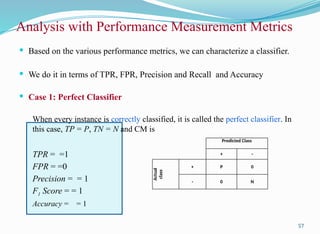
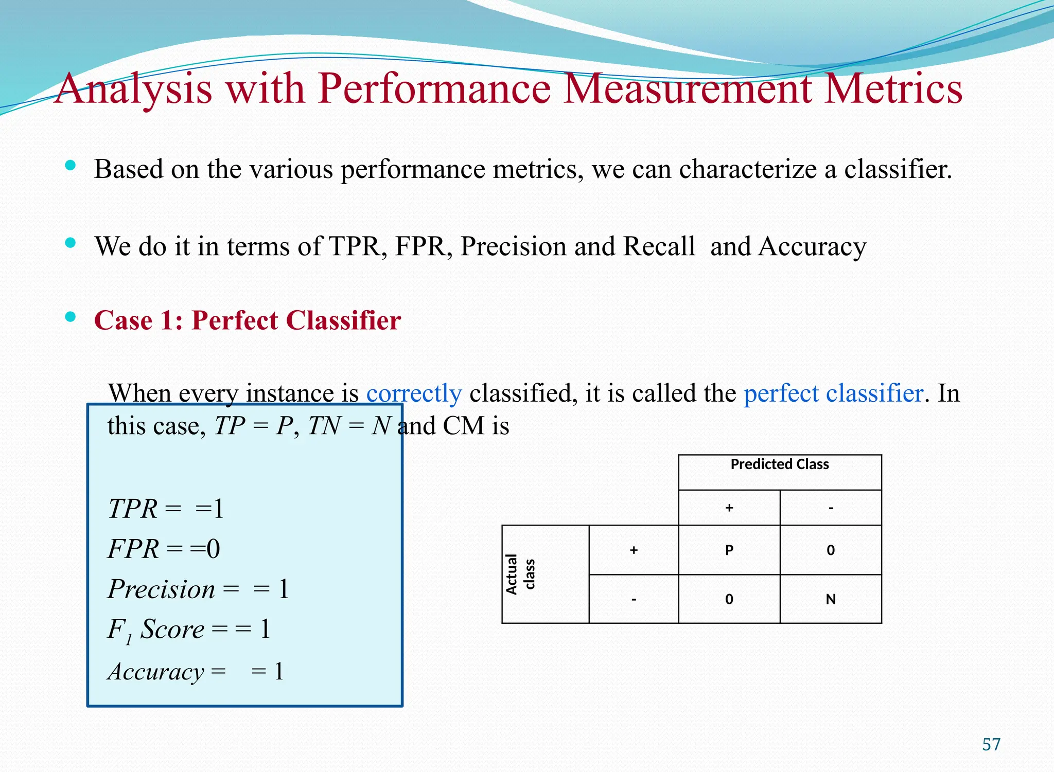
Analysis with PerformanceMeasurement Metrics
Based on the various performance metrics, we can characterize a classifier.
We do it in terms of TPR, FPR, Precision and Recall and Accuracy
Case 1: Perfect Classifier
When every instance is correctly classified, it is called the perfect classifier. In
this case, TP = P, TN = N and CM is
TPR = =1
FPR = =0
Precision = = 1
F1 Score = = 1
Accuracy = = 1
57
Predicted Class
+ -
Actual
class
+ P 0
- 0 N
58.
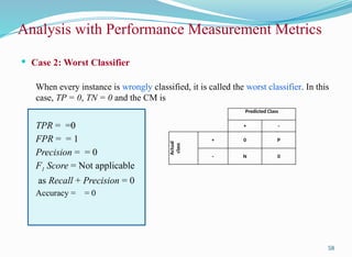
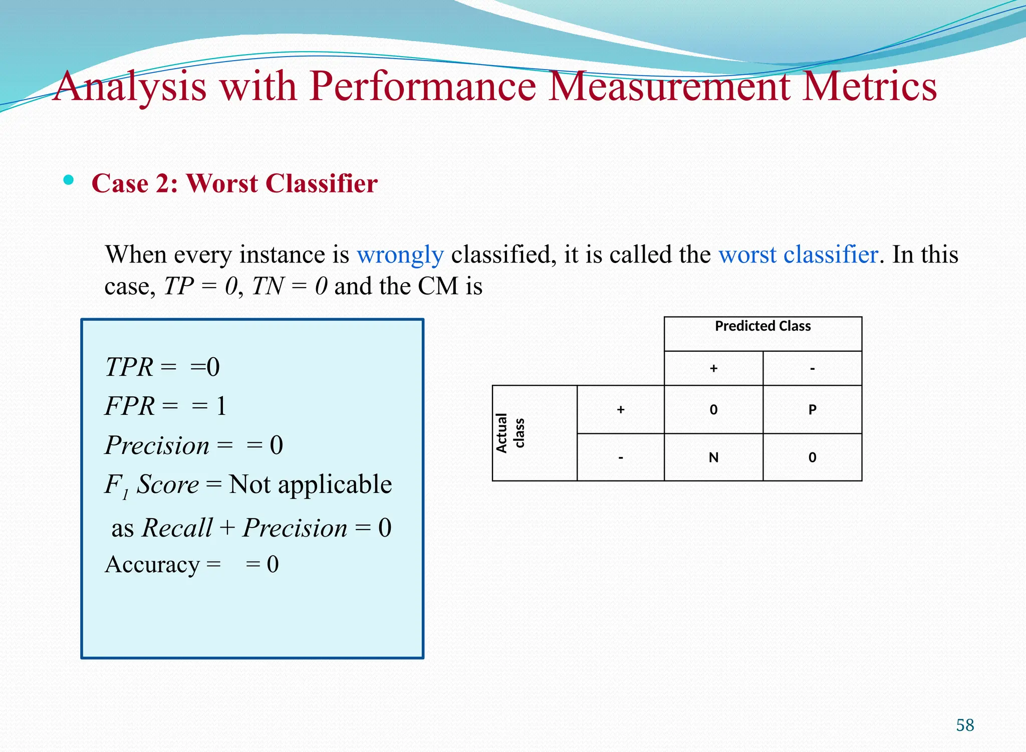
Analysis with PerformanceMeasurement Metrics
Case 2: Worst Classifier
When every instance is wrongly classified, it is called the worst classifier. In this
case, TP = 0, TN = 0 and the CM is
TPR = =0
FPR = = 1
Precision = = 0
F1 Score = Not applicable
as Recall + Precision = 0
Accuracy = = 0
58
Predicted Class
+ -
Actual
class
+ 0 P
- N 0
59.
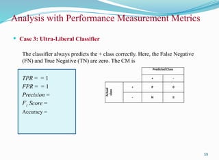
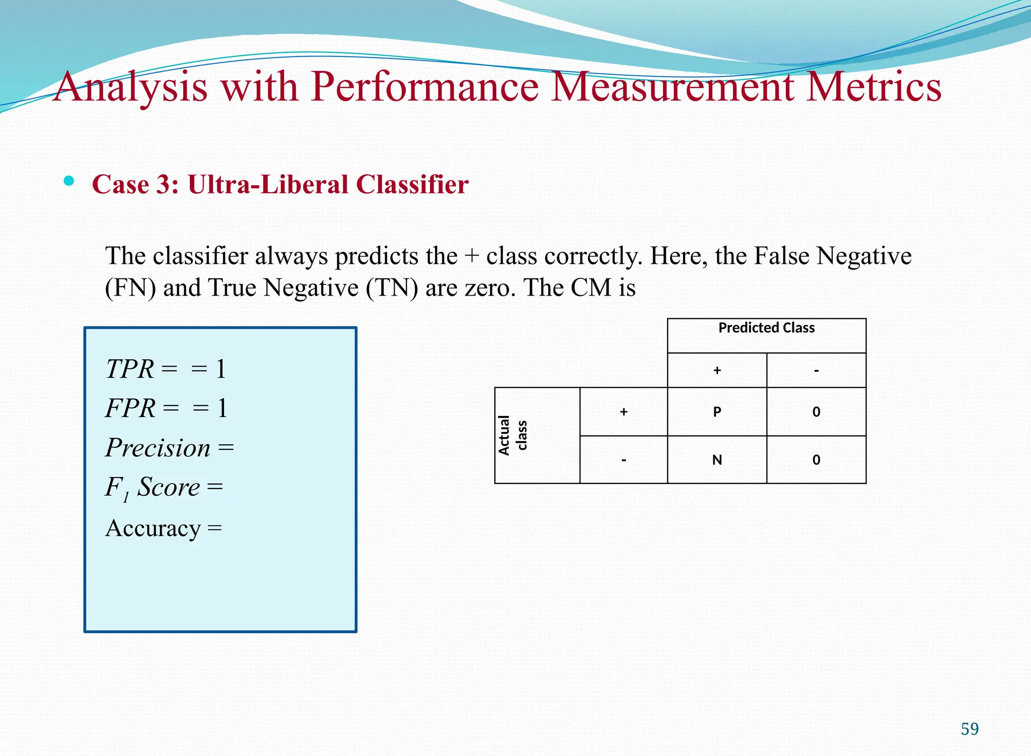
Analysis with PerformanceMeasurement Metrics
Case 3: Ultra-Liberal Classifier
The classifier always predicts the + class correctly. Here, the False Negative
(FN) and True Negative (TN) are zero. The CM is
TPR = = 1
FPR = = 1
Precision =
F1 Score =
Accuracy =
59
Predicted Class
+ -
Actual
class
+ P 0
- N 0
60.
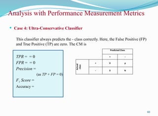
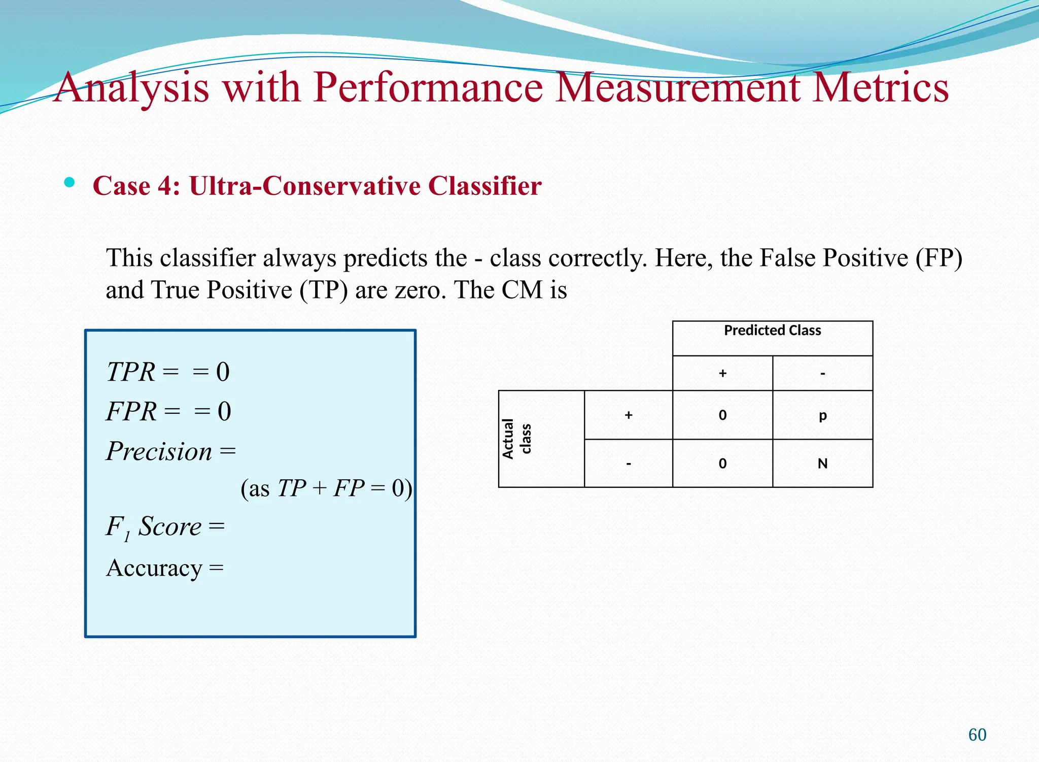
Analysis with PerformanceMeasurement Metrics
Case 4: Ultra-Conservative Classifier
This classifier always predicts the - class correctly. Here, the False Positive (FP)
and True Positive (TP) are zero. The CM is
TPR = = 0
FPR = = 0
Precision =
(as TP + FP = 0)
F1 Score =
Accuracy =
60
Predicted Class
+ -
Actual
class
+ 0 p
- 0 N
61.
Predictive Accuracy versusTPR and FPR
One strength of characterizing a classifier by its TPR and FPR is that they do
not depend on the relative size of P and N.
The same is also applicable for FNR and TNR and others measures from CM.
In contrast, the Predictive Accuracy, Precision, Error Rate, F1 Score, etc. are
affected by the relative size of P and N.
FPR, TPR, FNR and TNR are calculated from the different rows of the CM.
On the other hand Predictive Accuracy, etc. are derived from the values in both
rows.
This suggests that FPR, TPR, FNR and TNR are more effective than
Predictive Accuracy, etc.
61
ROC Curves
ROCis an abbreviation of Receiver Operating Characteristic come from the
signal detection theory, developed during World War 2 for analysis of radar
images.
In the context of classifier, ROC plot is a useful tool to study the behaviour of
a classifier or comparing two or more classifiers.
A ROC plot is a two-dimensional graph, where, X-axis represents FP rate
(FPR) and Y-axis represents TP rate (TPR).
Since, the values of FPR and TPR varies from 0 to 1 both inclusive, the two
axes thus from 0 to 1 only.
Each point (x, y) on the plot indicating that the FPR has value x and the TPR
value y.
63
64.
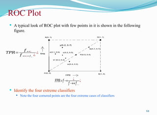
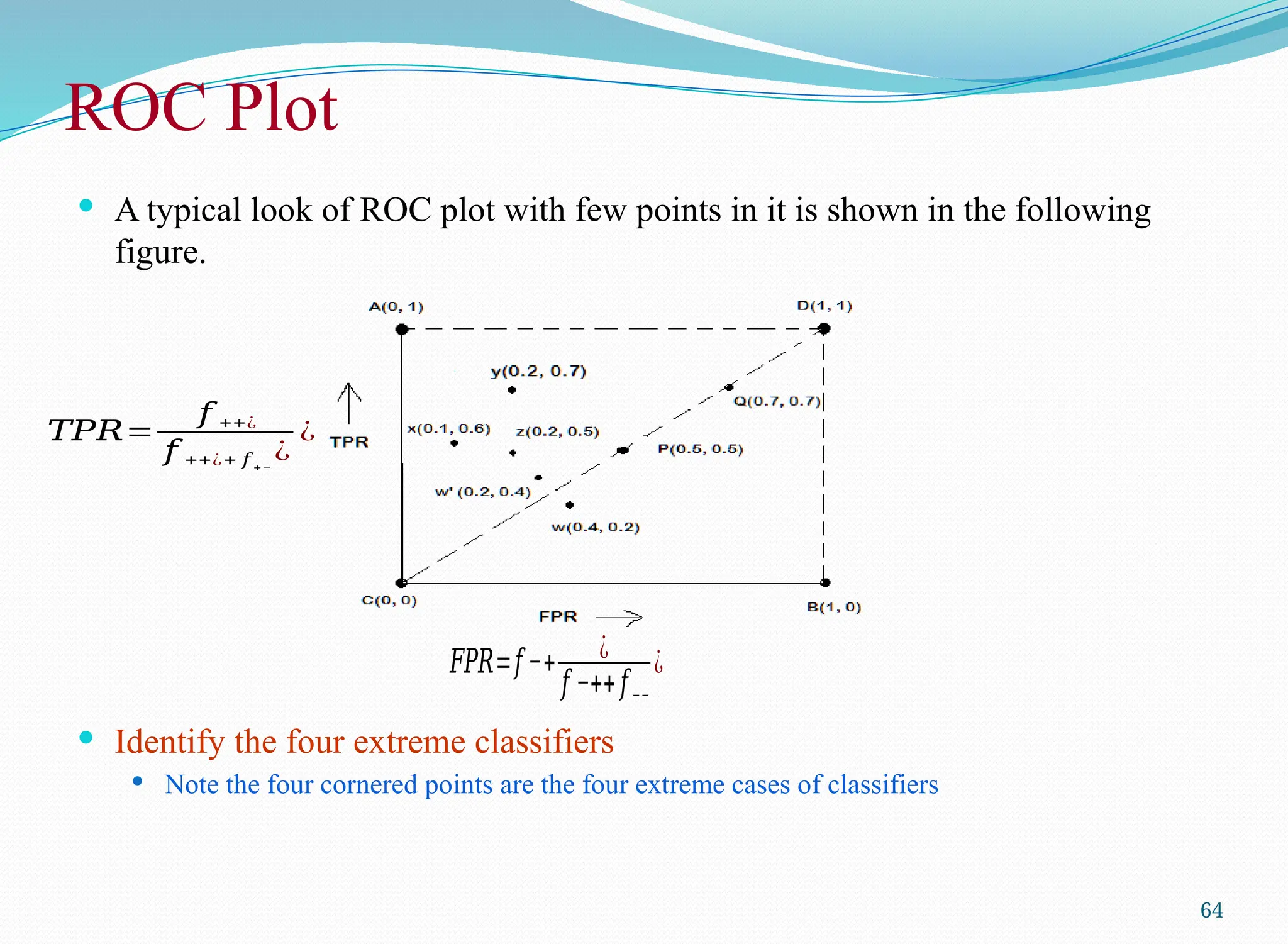
ROC Plot
Atypical look of ROC plot with few points in it is shown in the following
figure.
Identify the four extreme classifiers
Note the four cornered points are the four extreme cases of classifiers
64
𝑇𝑃𝑅=
𝑓 ++¿
𝑓 ++¿+ 𝑓 +−
¿
¿
𝐹𝑃𝑅=𝑓 −+ ¿
𝑓 −++𝑓−−
¿
65.
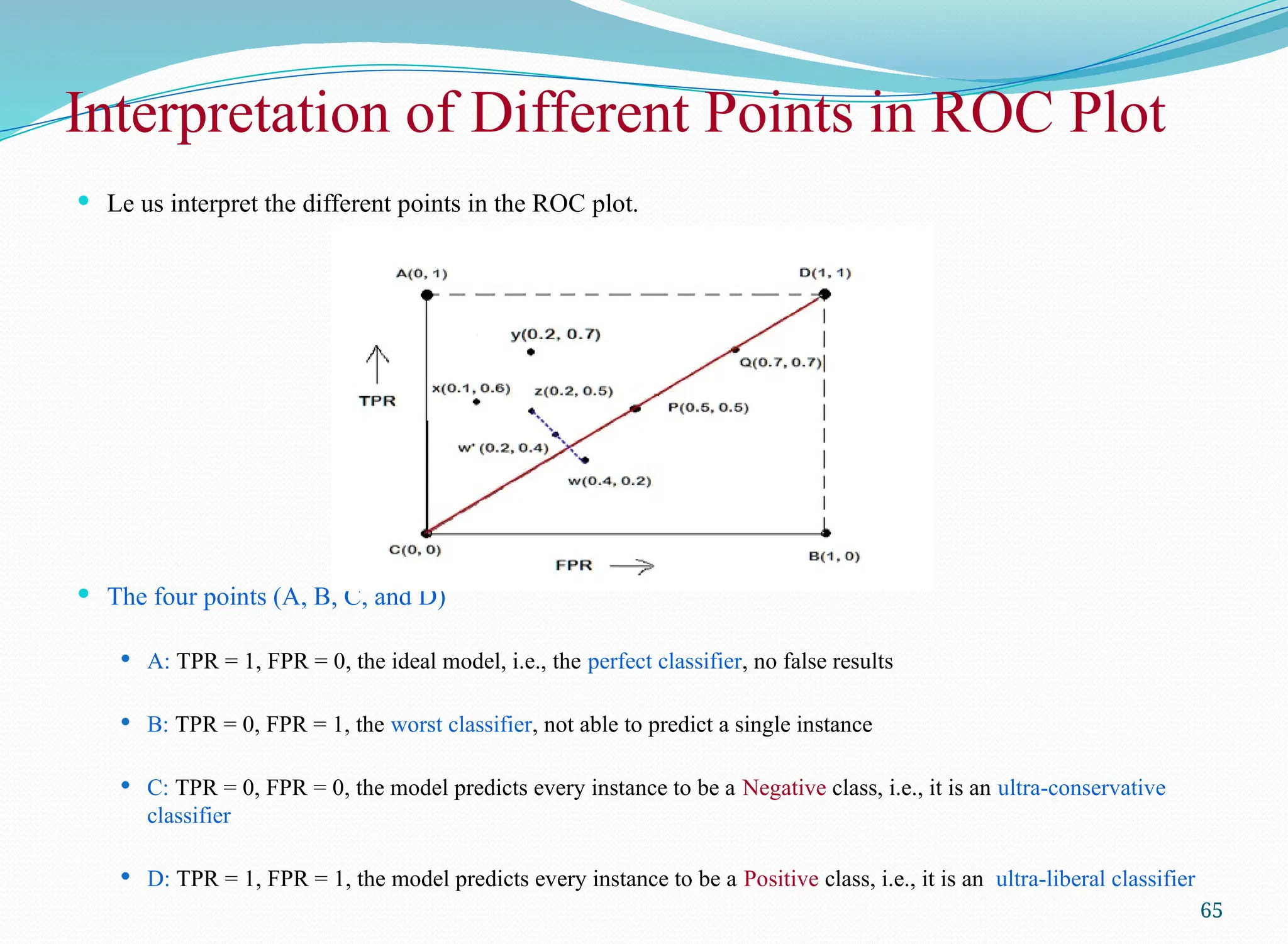
Interpretation of DifferentPoints in ROC Plot
Le us interpret the different points in the ROC plot.
The four points (A, B, C, and D)
A: TPR = 1, FPR = 0, the ideal model, i.e., the perfect classifier, no false results
B: TPR = 0, FPR = 1, the worst classifier, not able to predict a single instance
C: TPR = 0, FPR = 0, the model predicts every instance to be a Negative class, i.e., it is an ultra-conservative
classifier
D: TPR = 1, FPR = 1, the model predicts every instance to be a Positive class, i.e., it is an ultra-liberal classifier
65
66.
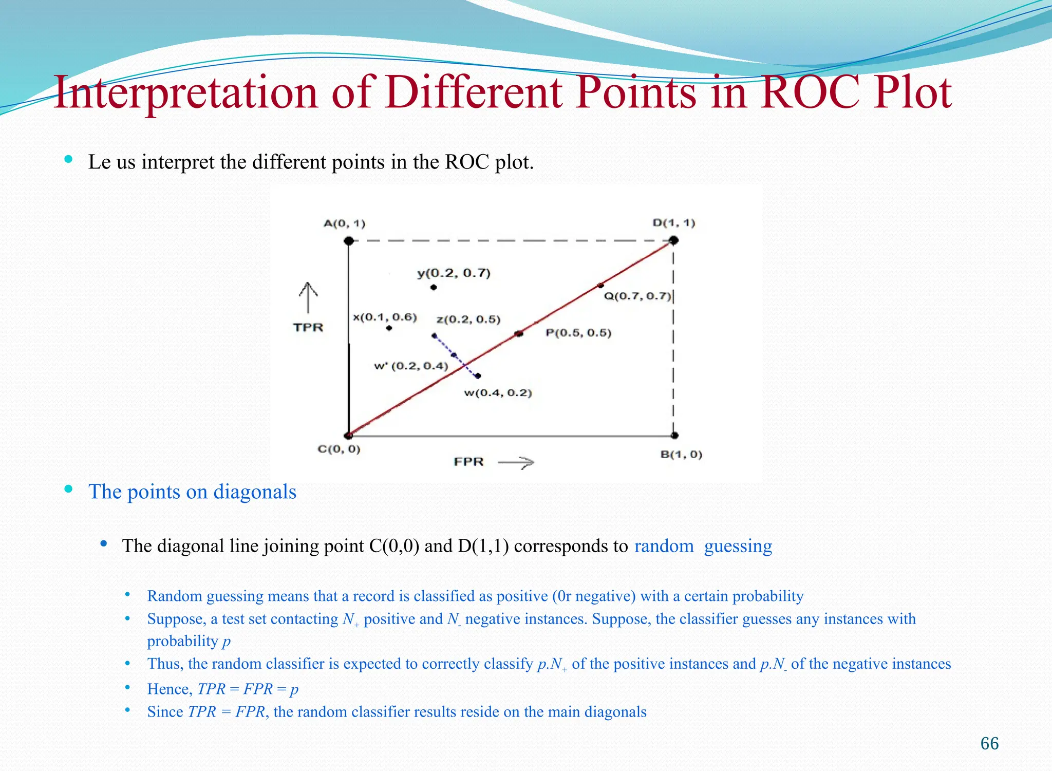
Interpretation of DifferentPoints in ROC Plot
Le us interpret the different points in the ROC plot.
The points on diagonals
The diagonal line joining point C(0,0) and D(1,1) corresponds to random guessing
Random guessing means that a record is classified as positive (0r negative) with a certain probability
Suppose, a test set contacting N+ positive and N- negative instances. Suppose, the classifier guesses any instances with
probability p
Thus, the random classifier is expected to correctly classify p.N+ of the positive instances and p.N- of the negative instances
Hence, TPR = FPR = p
Since TPR = FPR, the random classifier results reside on the main diagonals
66
67.
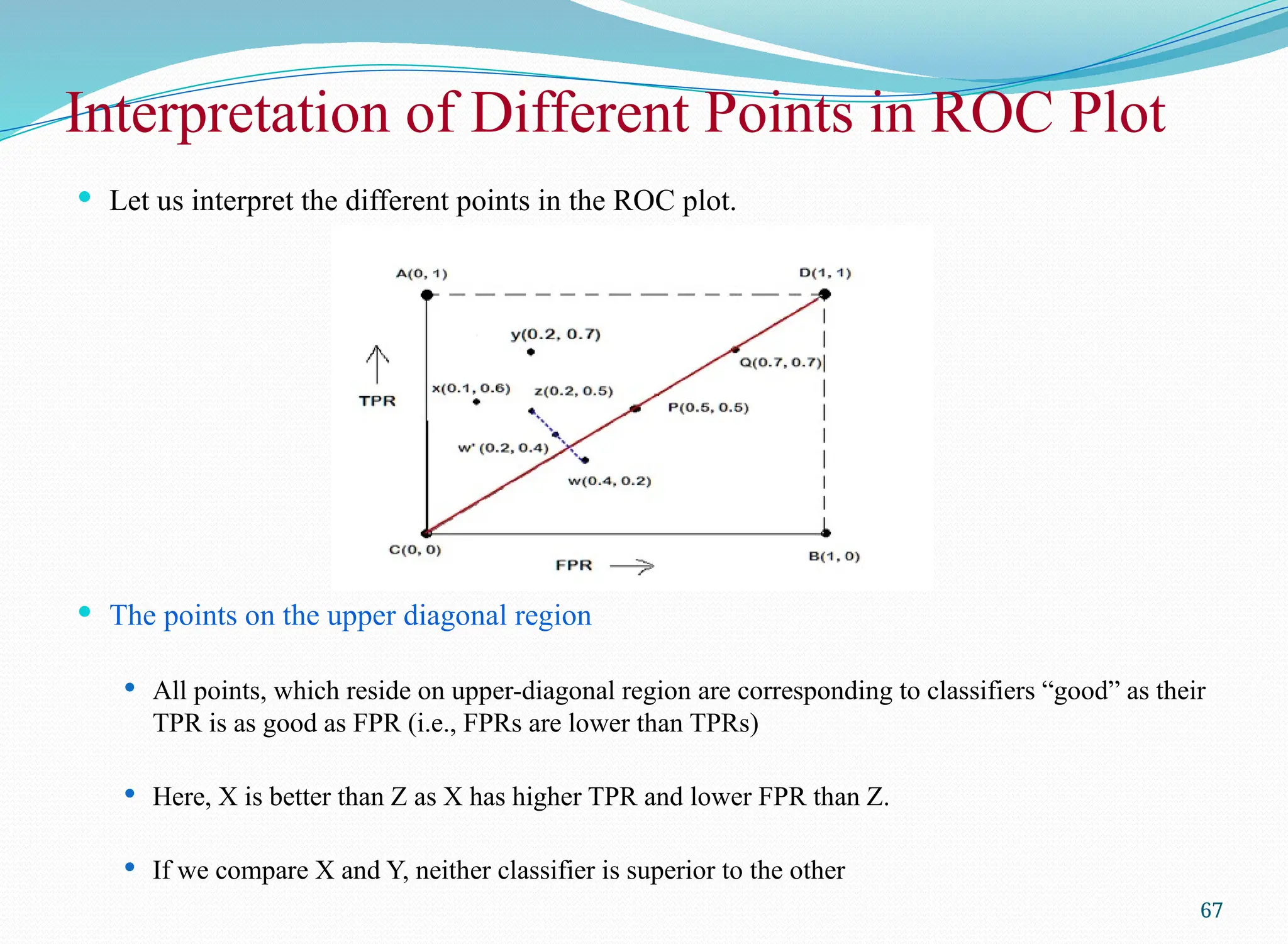
Interpretation of DifferentPoints in ROC Plot
Let us interpret the different points in the ROC plot.
The points on the upper diagonal region
All points, which reside on upper-diagonal region are corresponding to classifiers “good” as their
TPR is as good as FPR (i.e., FPRs are lower than TPRs)
Here, X is better than Z as X has higher TPR and lower FPR than Z.
If we compare X and Y, neither classifier is superior to the other
67
68.
Interpretation of DifferentPoints in ROC Plot
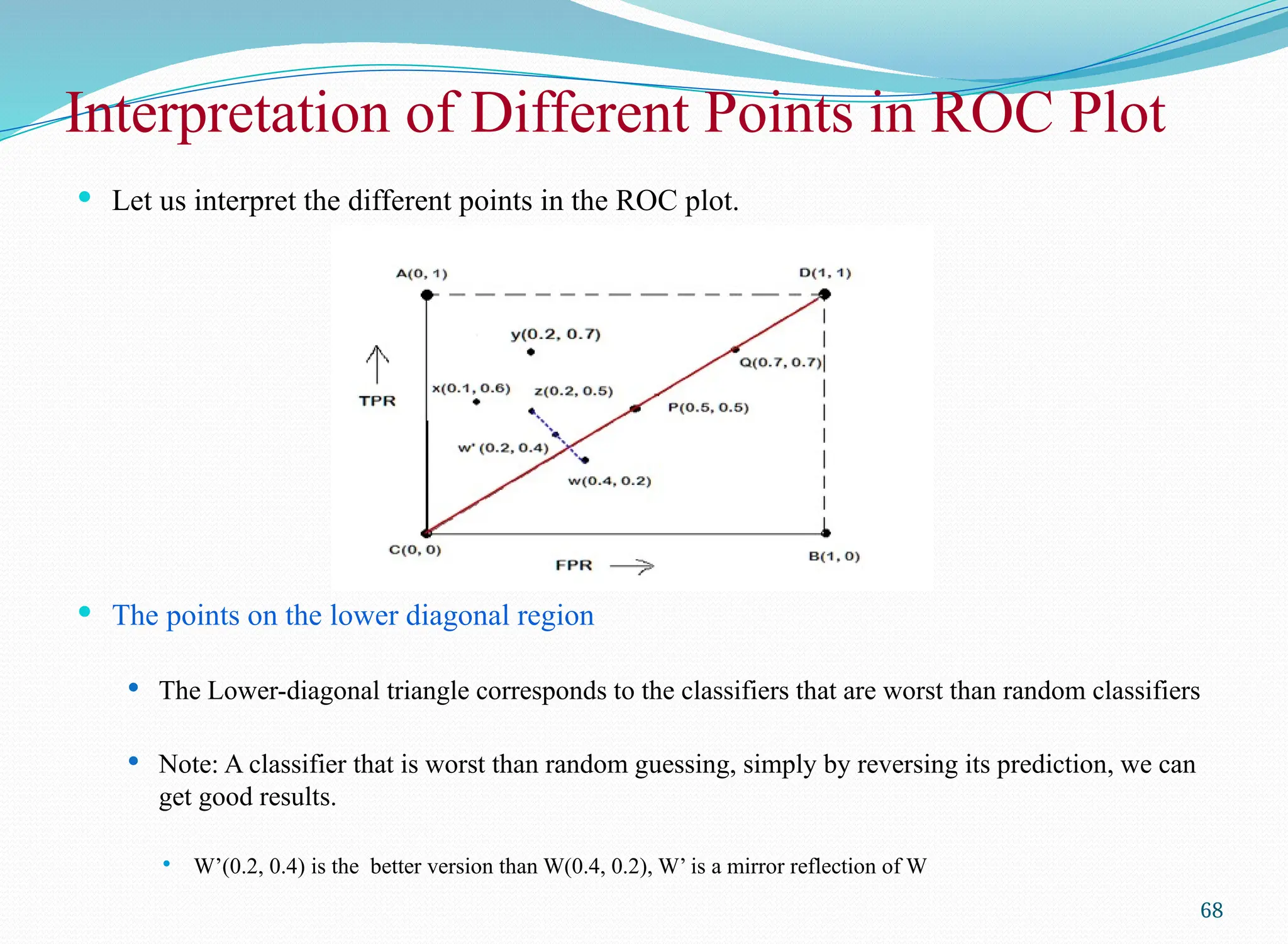
Let us interpret the different points in the ROC plot.
The points on the lower diagonal region
The Lower-diagonal triangle corresponds to the classifiers that are worst than random classifiers
Note: A classifier that is worst than random guessing, simply by reversing its prediction, we can
get good results.
W’(0.2, 0.4) is the better version than W(0.4, 0.2), W’ is a mirror reflection of W
68
69.
Tuning a Classifierthrough ROC Plot
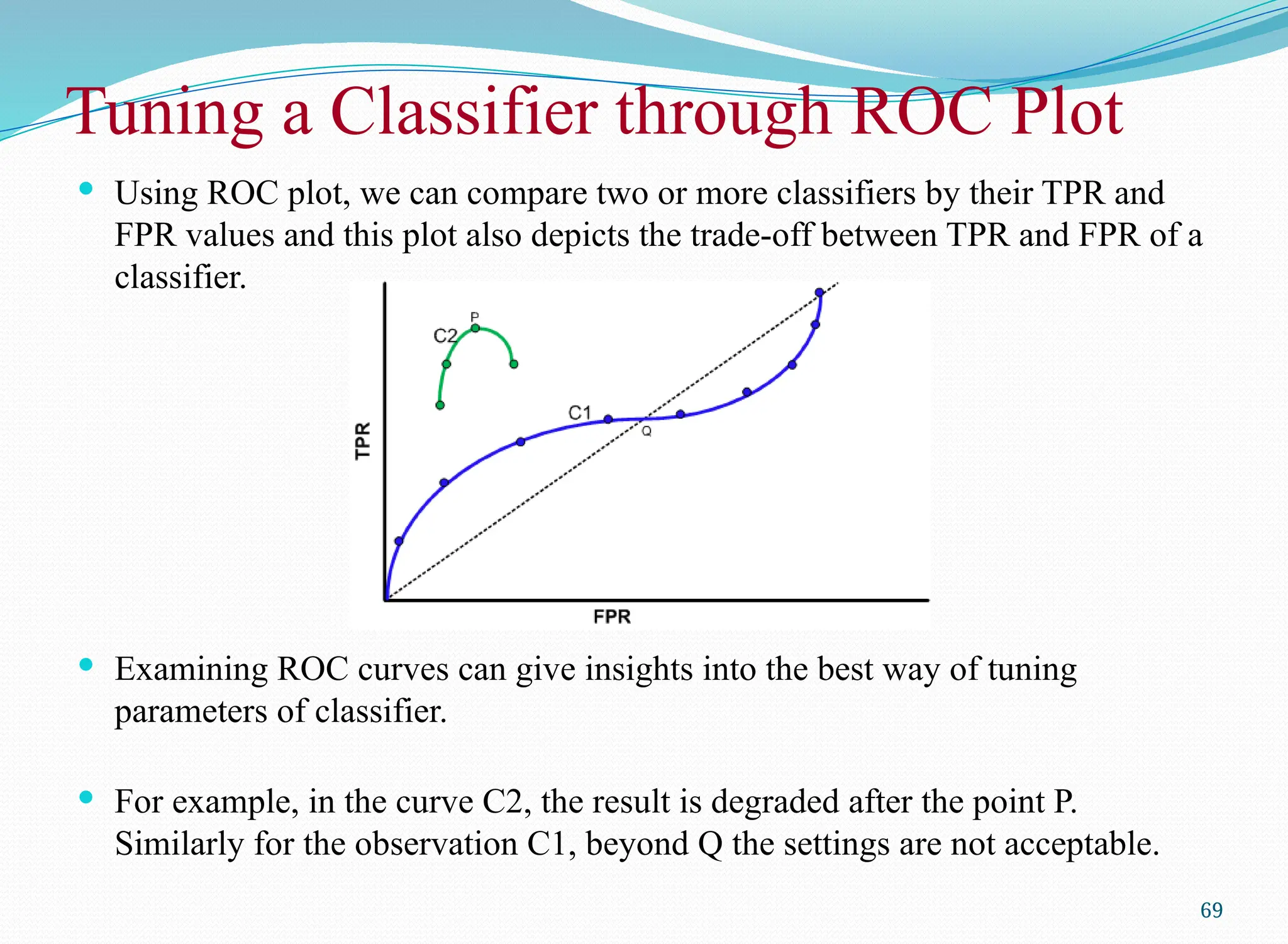
Using ROC plot, we can compare two or more classifiers by their TPR and
FPR values and this plot also depicts the trade-off between TPR and FPR of a
classifier.
Examining ROC curves can give insights into the best way of tuning
parameters of classifier.
For example, in the curve C2, the result is degraded after the point P.
Similarly for the observation C1, beyond Q the settings are not acceptable.
69
70.
Comparing Classifiers troughROC Plot
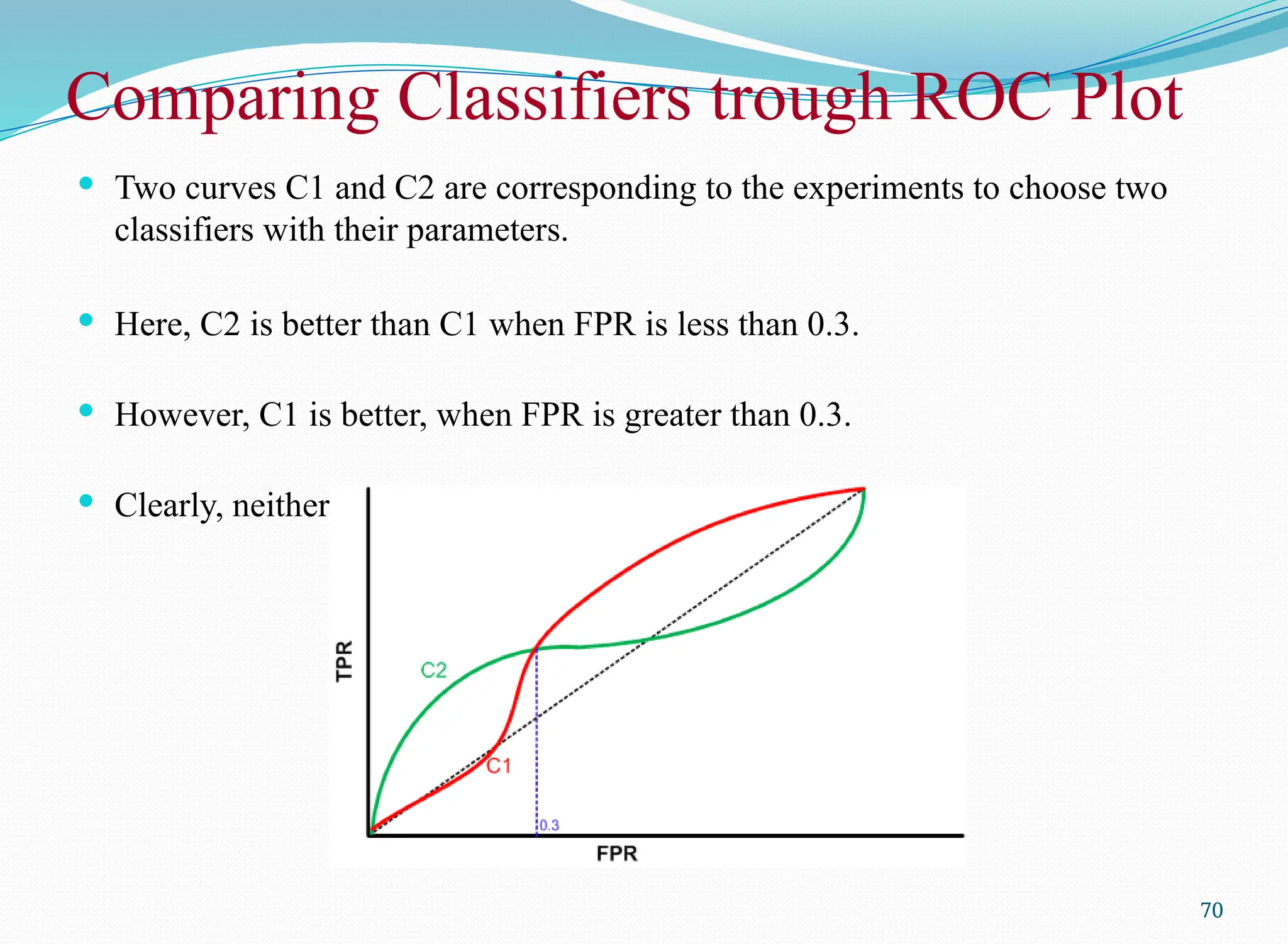
Two curves C1 and C2 are corresponding to the experiments to choose two
classifiers with their parameters.
Here, C2 is better than C1 when FPR is less than 0.3.
However, C1 is better, when FPR is greater than 0.3.
Clearly, neither of these two classifiers dominates the other.
70
71.
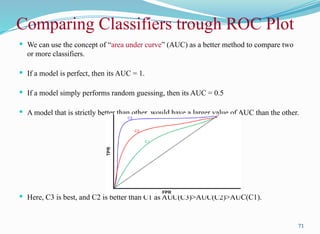
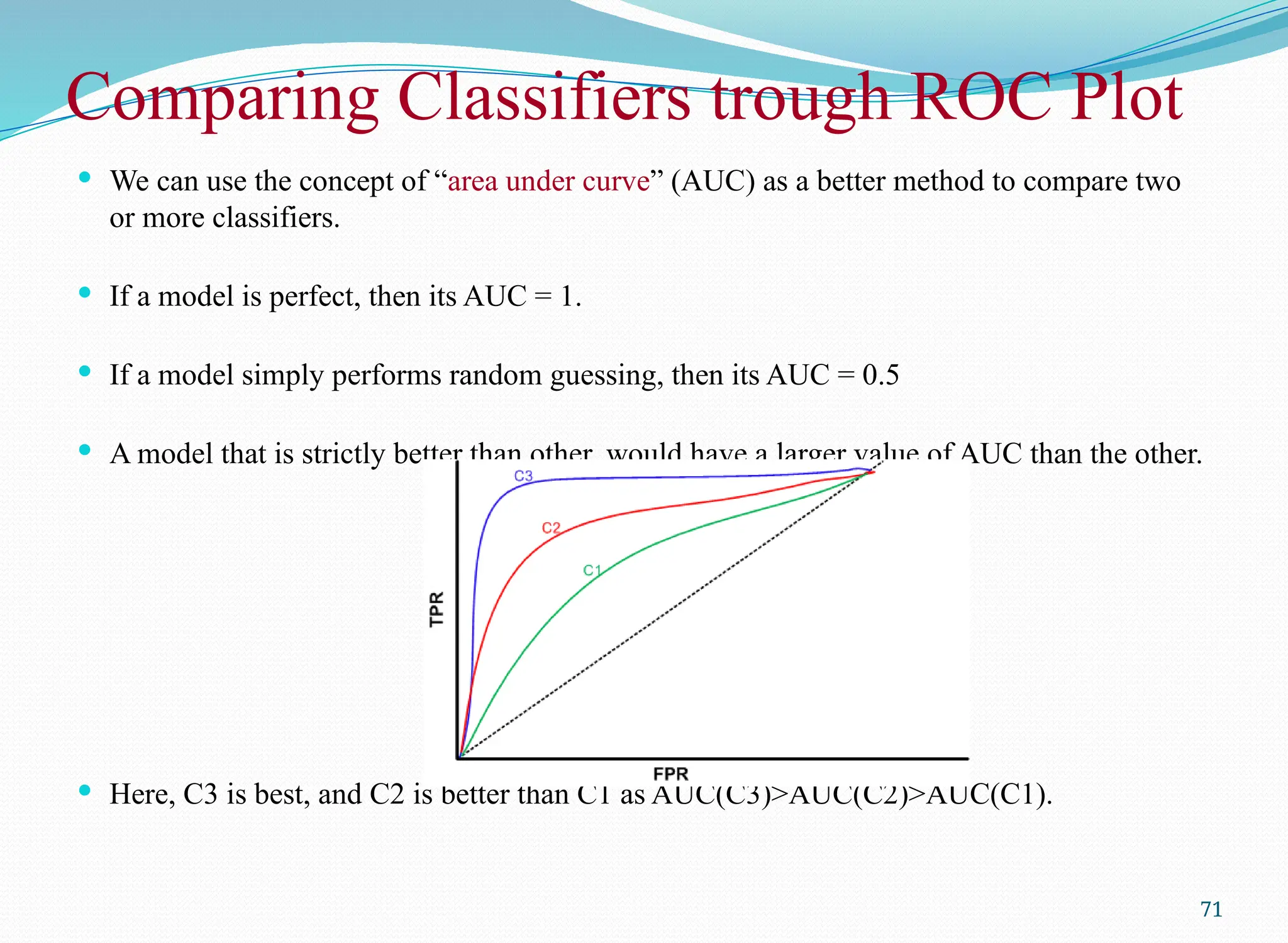
We canuse the concept of “area under curve” (AUC) as a better method to compare two
or more classifiers.
If a model is perfect, then its AUC = 1.
If a model simply performs random guessing, then its AUC = 0.5
A model that is strictly better than other, would have a larger value of AUC than the other.
Here, C3 is best, and C2 is better than C1 as AUC(C3)>AUC(C2)>AUC(C1).
71
Comparing Classifiers trough ROC Plot
72.
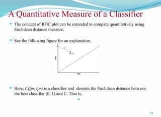
A Quantitative Measureof a Classifier
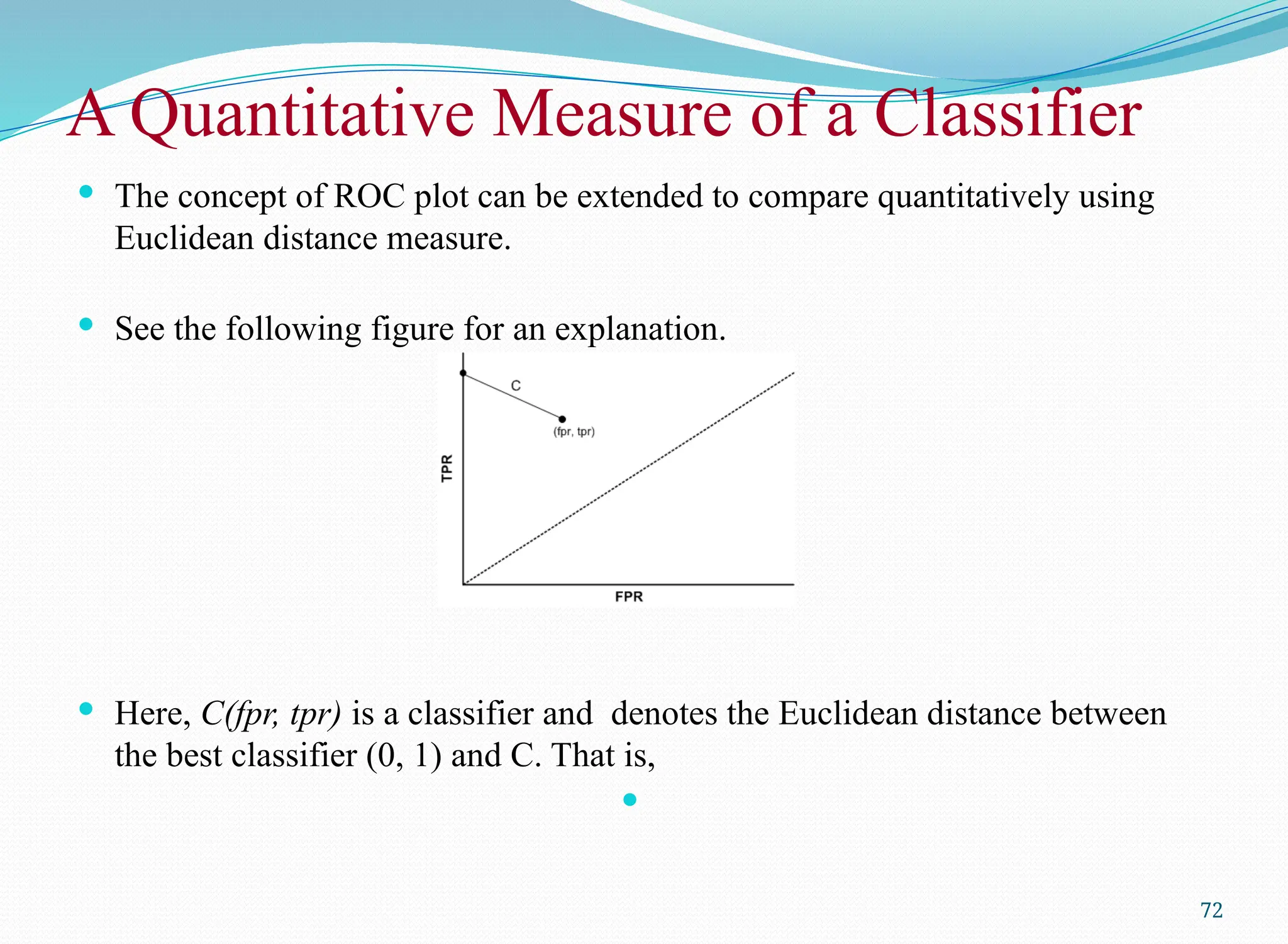
The concept of ROC plot can be extended to compare quantitatively using
Euclidean distance measure.
See the following figure for an explanation.
Here, C(fpr, tpr) is a classifier and denotes the Euclidean distance between
the best classifier (0, 1) and C. That is,
72
73.
A Quantitative Measureof a Classifier
The smallest possible value of is 0
The largest possible values of i(when (fpr = 1 and tpr = 0).
We could hypothesise that the smaller the value of , the better the classifier.
is a useful measure, but does not take into account the relative importance of true and false positive
rates.
We can specify the relative importance of making TPR as close to 1 and FPR as close 0 by a weight w
between 0 to 1.
We can define weighted (denoted by ) as
Note
If w = 0, it reduces to = fpr, i.e., FP Rate.
If w = 1, it reduces to = 1 – tpr, i.e., we are only interested to maximizing TP Rate.
73
74.
Reference
74
The detailmaterial related to this lecture can be found in
Data Mining: Concepts and Techniques, (3rd
Edn.), Jiawei Han, Micheline Kamber,
Morgan Kaufmann, 2015.
Introduction to Data Mining, Pang-Ning Tan, Michael Steinbach, and Vipin Kumar,
Addison-Wesley, 2014