Download to read offline


![Problem 4.
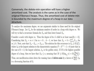
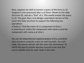
The least common ancestor (sometimes called lowest common
ancestor) of nodes v and w in an n node rooted tree T is the node
furthest from the root that is an ancestor of both v and w. The
following algorithm solves the offline problem. That is, given a set
of query pairs, it computes all of the answers quickly. It makes use a
unionfind data structure. You may want to review this data
structure (cf. [CLRS], Chapter 21), and in particular the union
by
rank heuristic. Offline LCA: Associate with each node an extra field
“name”. Process the nodes of T in post order. To process a node,
consider all of the query pairs it is a member of. For each pair, if the
other endpoint has not yet been processed, do nothing. If the other
endpoint has been processed do a find on it, and record the
“name” of the result as the LCA of this pair. After considering all of
the pairs, union the node with its parent, and set the “name” of the
set representative to be the parent](https://image.slidesharecdn.com/ppt05-240812114721-bfd38455/85/RProgrammingassignmenthPPT_05-07-24-pptx-11-320.jpg)

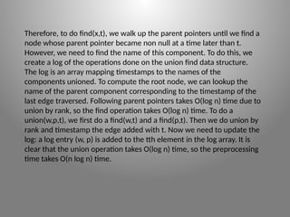


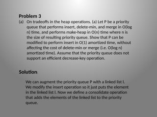
![Problem 4.
The least common ancestor (sometimes called lowest common
ancestor) of nodes v and w in an n node rooted tree T is the node
furthest from the root that is an ancestor of both v and w. The
following algorithm solves the offline problem. That is, given a set
of query pairs, it computes all of the answers quickly. It makes use a
unionfind data structure. You may want to review this data
structure (cf. [CLRS], Chapter 21), and in particular the union
by
rank heuristic. Offline LCA: Associate with each node an extra field
“name”. Process the nodes of T in post order. To process a node,
consider all of the query pairs it is a member of. For each pair, if the
other endpoint has not yet been processed, do nothing. If the other
endpoint has been processed do a find on it, and record the
“name” of the result as the LCA of this pair. After considering all of
the pairs, union the node with its parent, and set the “name” of the
set representative to be the parent](https://image.slidesharecdn.com/ppt05-240812114721-bfd38455/75/RProgrammingassignmenthPPT_05-07-24-pptx-11-2048.jpg)

The document presents an advanced algorithms assignment focused on R programming, detailing solutions and analyses regarding Fibonacci heaps, priority queues, and least common ancestors in trees. It discusses various problems, providing step-by-step explanations and modifications to improve operations while maintaining efficiency. The document also emphasizes the use of persistent data structures for efficiently answering least common ancestor queries online.