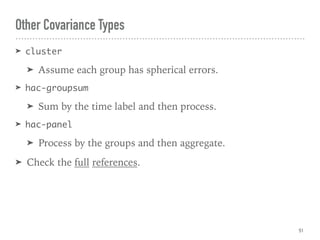
Download as PDF, PPTX
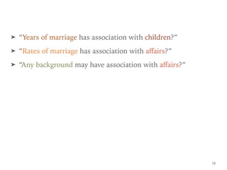
![Define Assumptions
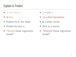
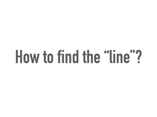
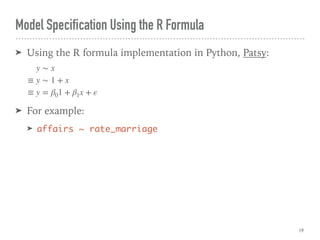
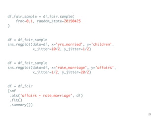
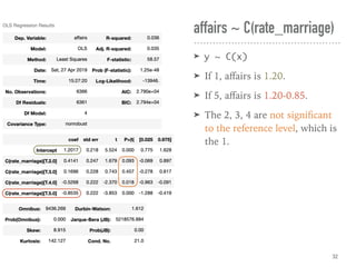
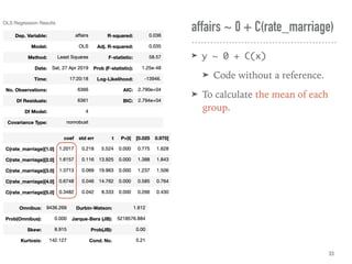
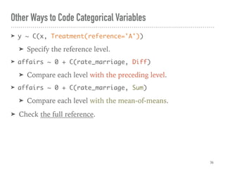
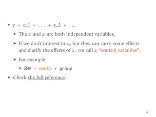
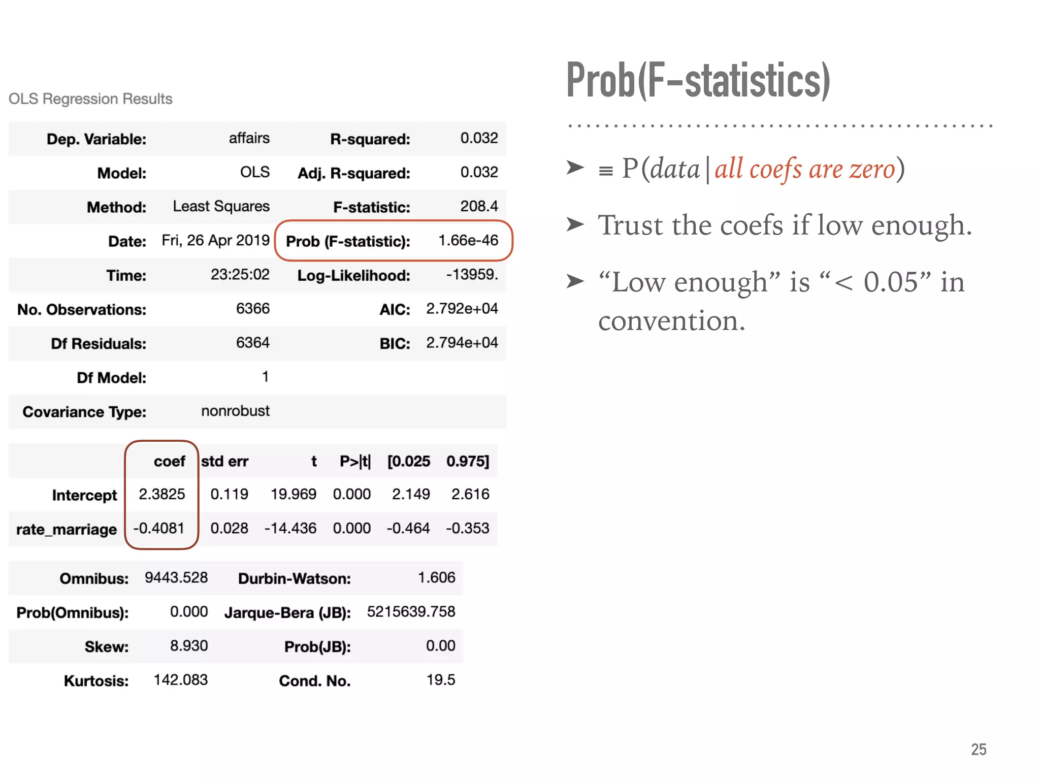
➤ The regression analysis:
➤ Suitable to measure the relationship between variables.
➤ Can model most of the hypothesis testing. [ref]
➤ Can predict.
9](https://image.slidesharecdn.com/statisticalregressionwithpython-190511114627/85/Statistical-Regression-With-Python-9-320.jpg)
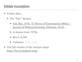

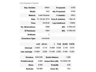
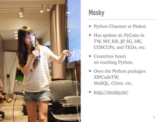
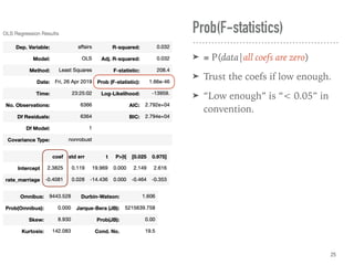
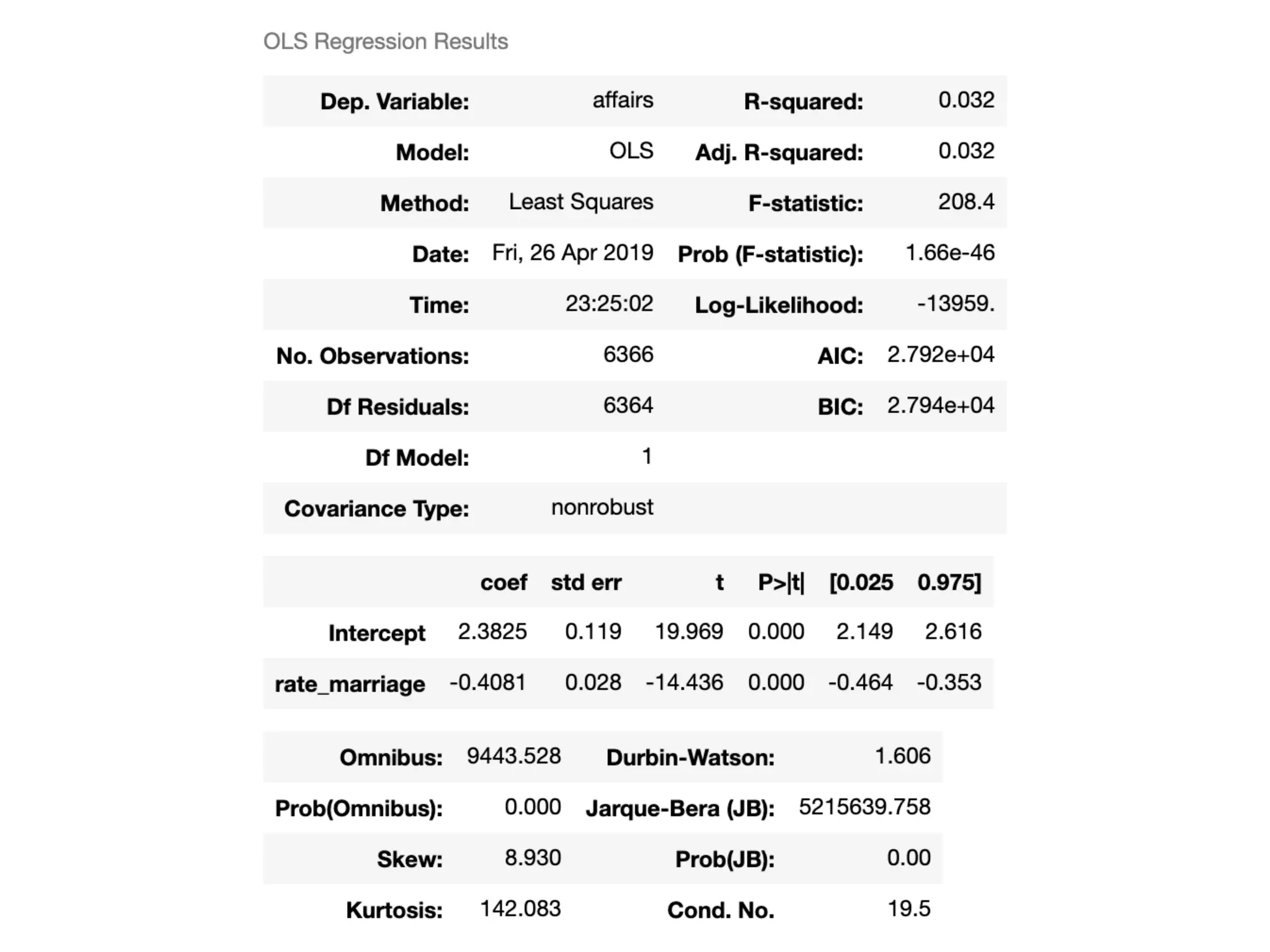
![Adj. R-squared
➤ ≡ explained var. by X / var. of y
and adjusted by no. of X
➤ ∈ [0, 1], usually.
➤ Can compare among models.
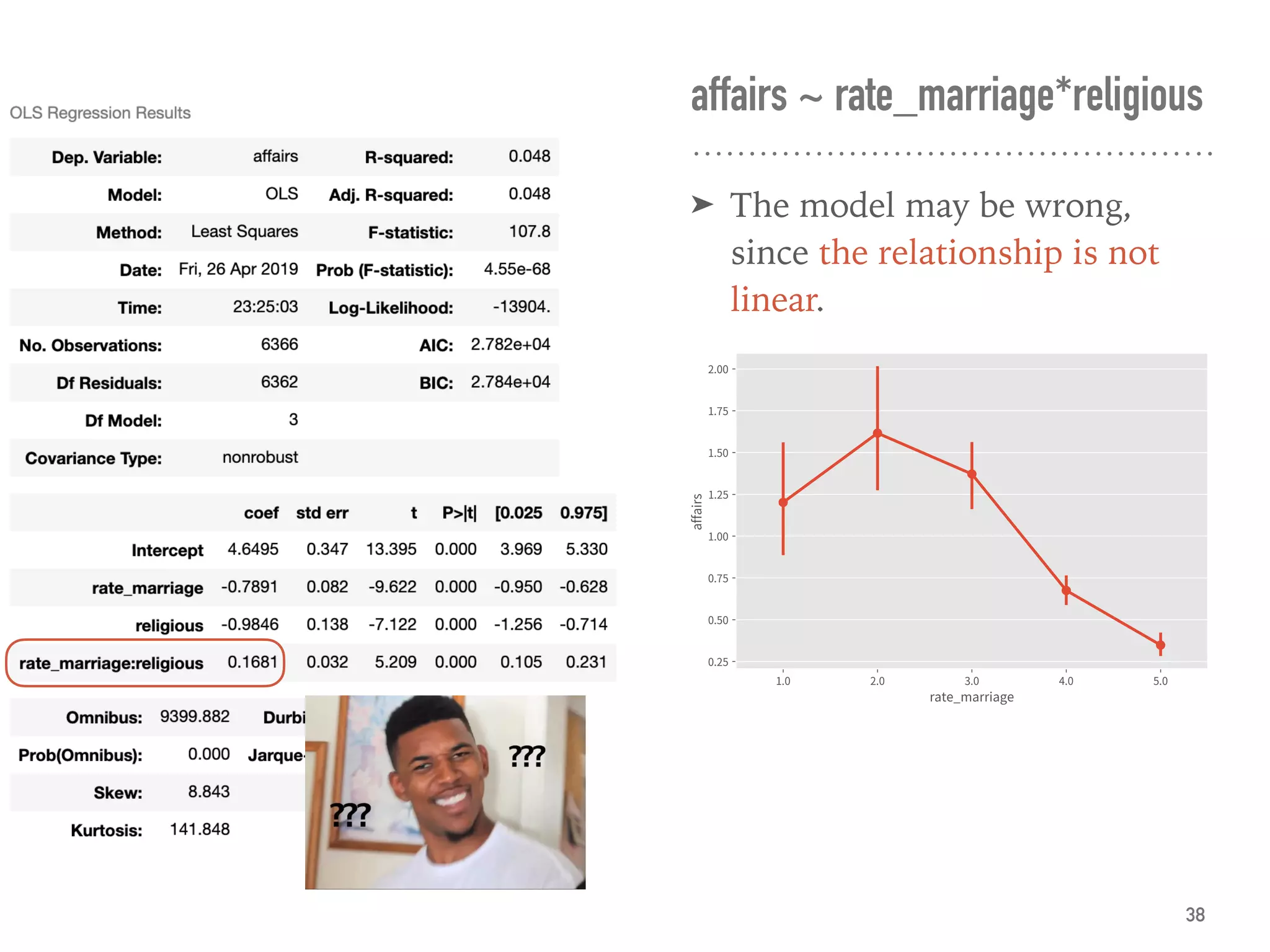
➤ 0.032 is super bad.
24](https://image.slidesharecdn.com/statisticalregressionwithpython-190511114627/85/Statistical-Regression-With-Python-24-320.jpg)
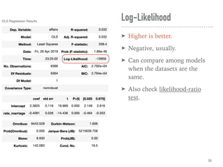
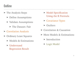
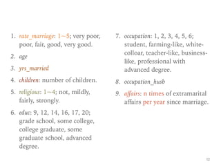
![Large Sample or Normality
➤ No. Observations, or
➤ ≥ 110~200 [ref]
➤ Normality of Residuals
➤ Prob(Omnibus) ≥ 0.05
➤ ∧ Prob(JB) ≥ 0.05
➤ To construct interval estimates
correctly, e.g., hypothesis tests
on coefs, confidence intervals.
27](https://image.slidesharecdn.com/statisticalregressionwithpython-190511114627/85/Statistical-Regression-With-Python-27-320.jpg)

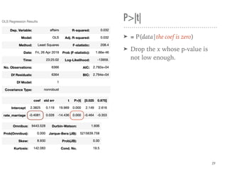
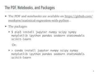
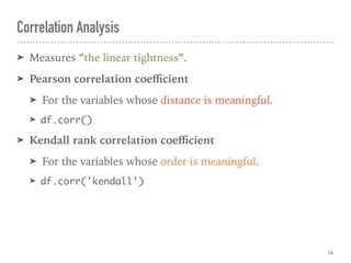
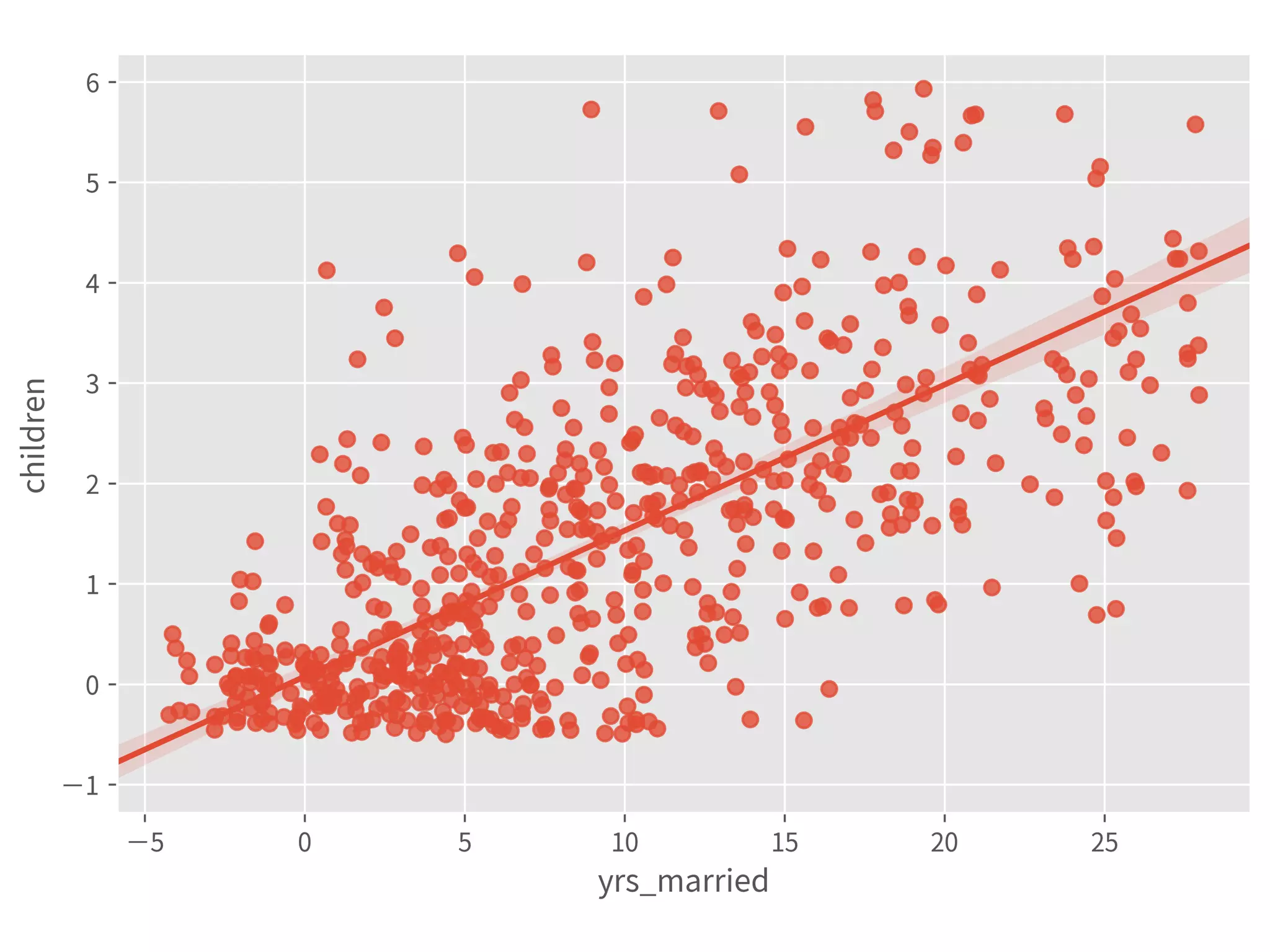
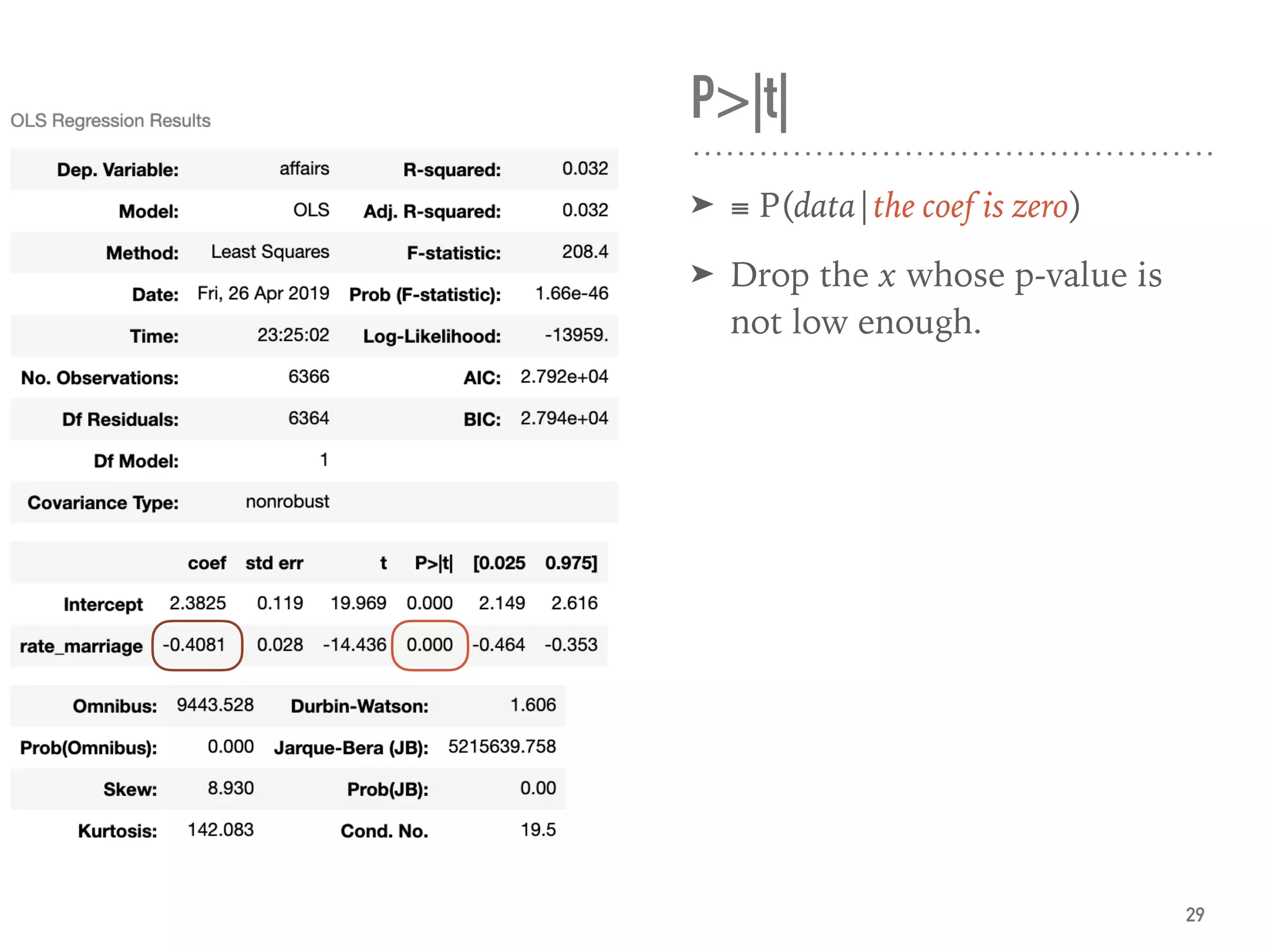
![Coef & Confidence Intervals
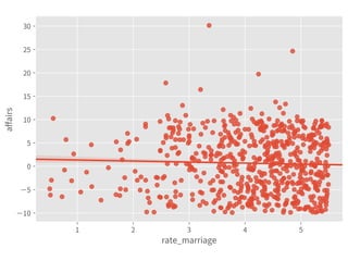
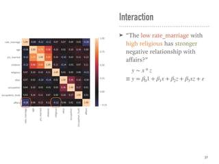
➤ “The rate_marriage and affairs
has negative relationship, the
strength is -0.41, and 95%
confidence interval is [-0.46,
-0.35].”
30](https://image.slidesharecdn.com/statisticalregressionwithpython-190511114627/85/Statistical-Regression-With-Python-30-320.jpg)


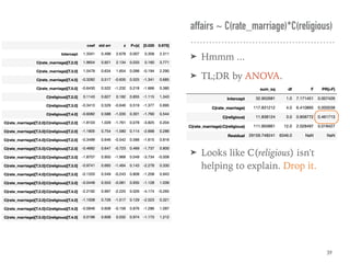
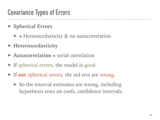
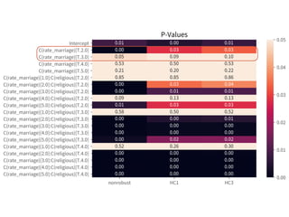
![➤ Use HC std errs
(heteroscedasticity-consistent
standard errors) to correct.
➤ If N ≤ 250, use HC3. [ref]
➤ If N > 250, consider HC1 for
the speed.
➤ Also suggest to use by default.
➤ .fit(cov_type='HC3')
← The confidence intervals
vary among groups. The
heteroscedasticity exists.
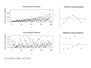
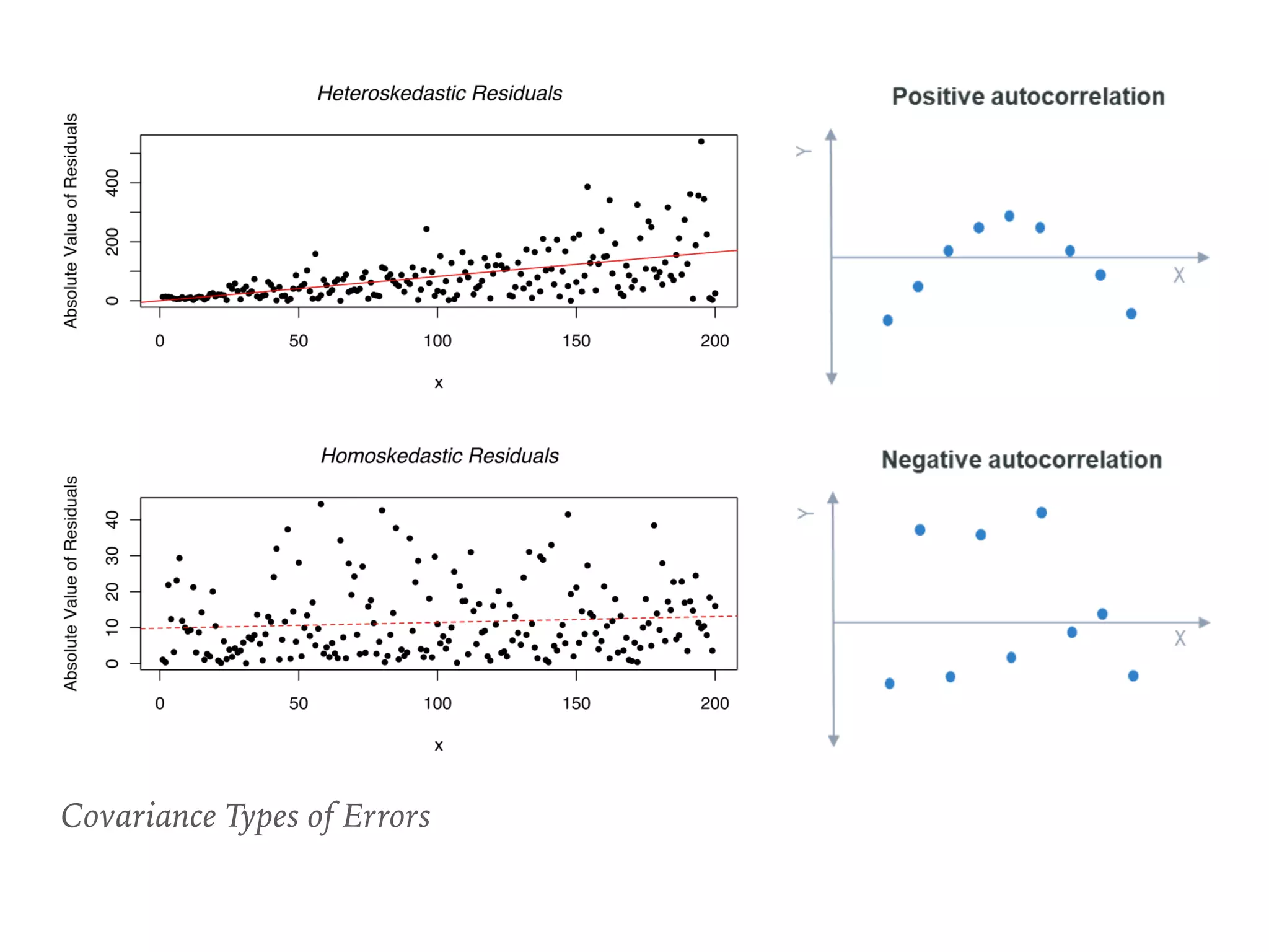
Heteroscedasticity
48](https://image.slidesharecdn.com/statisticalregressionwithpython-190511114627/85/Statistical-Regression-With-Python-48-320.jpg)
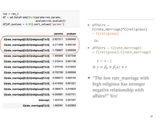
![Autocorrelation
➤ Durbin-Watson
➤ 2 is no autocorrelation.
➤ [0, 2) is positive
autocorrelation.
➤ (2, 4] is negative
autocorrelation.
➤ [1.5, 2.5] are relatively
normal. [ref]
➤ Use HAC std err.
➤ .fit(cov_type='HAC',
cov_kwds=dict(maxlag=tau))
50](https://image.slidesharecdn.com/statisticalregressionwithpython-190511114627/85/Statistical-Regression-With-Python-50-320.jpg)

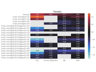
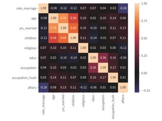
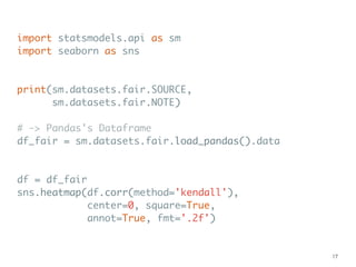
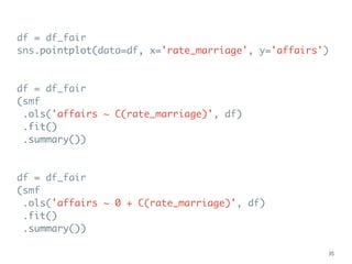
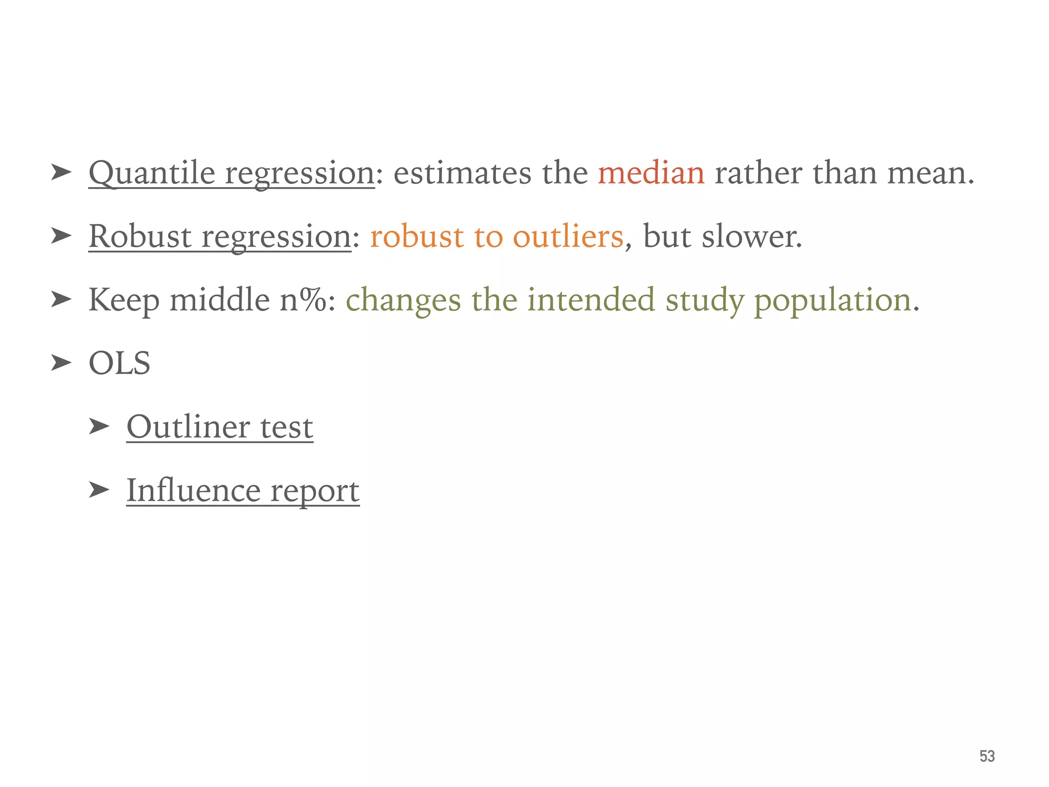
![df = df_fair
alpha = 0.05
a = df.affairs.quantile(alpha/2)
b = df.affairs.quantile(1-alpha/2)
df = df[(df.affairs >= a) & (df.affairs <= b)]
df_fair_middle95 = df
df = df_fair
smf.ols(formula, df).fit().summary()
smf.ols(formula, df_fair_middle95).fit().summary()
smf.quantreg(formula, df).fit().summary()
smf.rlm(formula, df).fit().summary()
55](https://image.slidesharecdn.com/statisticalregressionwithpython-190511114627/85/Statistical-Regression-With-Python-55-320.jpg)
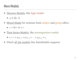
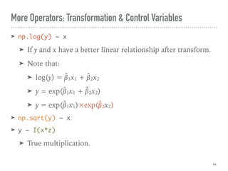
![More Estimations
➤ MLE, Maximum
Likelihood Estimation.
← Usually find by
numerical methods.
➤ TSLS, Two-Stage Least
Squares.
➤ y ← (x ← z)
➤ Handle the endogeneity:
E[ε|X] ≠ 0.
62](https://image.slidesharecdn.com/statisticalregressionwithpython-190511114627/85/Statistical-Regression-With-Python-62-320.jpg)
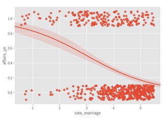
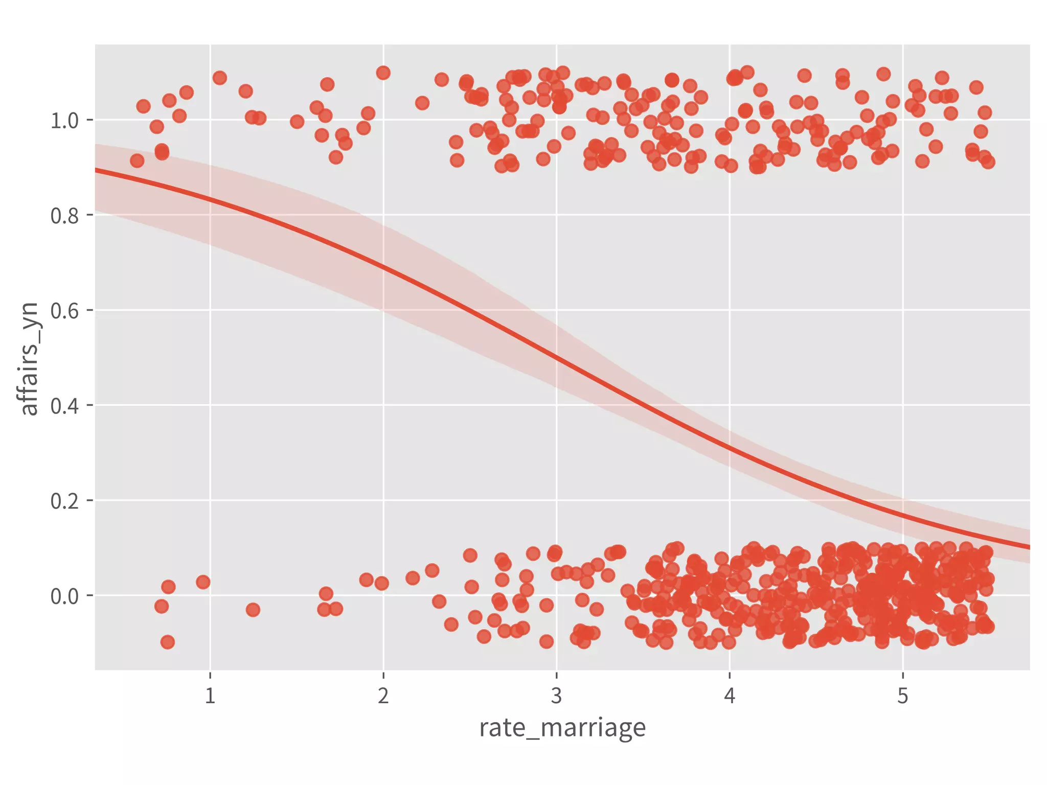
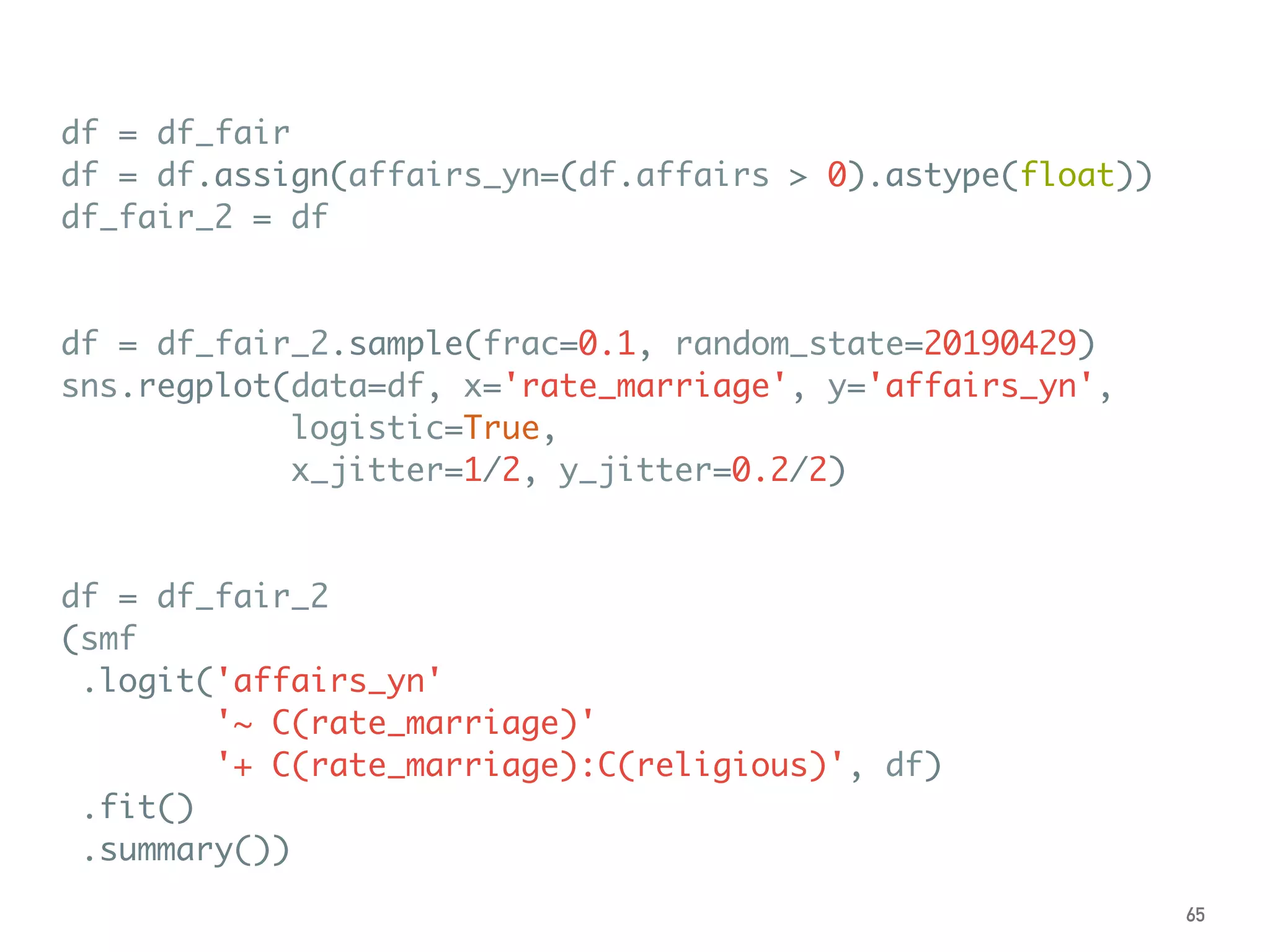
![Logit Model
➤ The coef is log-odds.
➤ Use exp(x)/(exp(x)+1) to
transform back to probability:
➤ 0.6931 → 67%
➤ ″ - 1.6664 → 27%
➤ ″ - 1.3503 → 9%
Or:
➤ .predict(dict(
rate_marriage=[1, 5, 5],
religious=[1, 1, 4]))
64](https://image.slidesharecdn.com/statisticalregressionwithpython-190511114627/85/Statistical-Regression-With-Python-64-320.jpg)

![Define Assumptions
➤ The regression analysis:
➤ Suitable to measure the relationship between variables.
➤ Can model most of the hypothesis testing. [ref]
➤ Can predict.
9](https://image.slidesharecdn.com/statisticalregressionwithpython-190511114627/75/Statistical-Regression-With-Python-9-2048.jpg)


![Adj. R-squared
➤ ≡ explained var. by X / var. of y
and adjusted by no. of X
➤ ∈ [0, 1], usually.
➤ Can compare among models.
➤ 0.032 is super bad.
24](https://image.slidesharecdn.com/statisticalregressionwithpython-190511114627/75/Statistical-Regression-With-Python-24-2048.jpg)
![Large Sample or Normality
➤ No. Observations, or
➤ ≥ 110~200 [ref]
➤ Normality of Residuals
➤ Prob(Omnibus) ≥ 0.05
➤ ∧ Prob(JB) ≥ 0.05
➤ To construct interval estimates
correctly, e.g., hypothesis tests
on coefs, confidence intervals.
27](https://image.slidesharecdn.com/statisticalregressionwithpython-190511114627/75/Statistical-Regression-With-Python-27-2048.jpg)
![Coef & Confidence Intervals
➤ “The rate_marriage and affairs
has negative relationship, the
strength is -0.41, and 95%
confidence interval is [-0.46,
-0.35].”
30](https://image.slidesharecdn.com/statisticalregressionwithpython-190511114627/75/Statistical-Regression-With-Python-30-2048.jpg)

![➤ Use HC std errs
(heteroscedasticity-consistent
standard errors) to correct.
➤ If N ≤ 250, use HC3. [ref]
➤ If N > 250, consider HC1 for
the speed.
➤ Also suggest to use by default.
➤ .fit(cov_type='HC3')
← The confidence intervals
vary among groups. The
heteroscedasticity exists.
Heteroscedasticity
48](https://image.slidesharecdn.com/statisticalregressionwithpython-190511114627/75/Statistical-Regression-With-Python-48-2048.jpg)

![Autocorrelation
➤ Durbin-Watson
➤ 2 is no autocorrelation.
➤ [0, 2) is positive
autocorrelation.
➤ (2, 4] is negative
autocorrelation.
➤ [1.5, 2.5] are relatively
normal. [ref]
➤ Use HAC std err.
➤ .fit(cov_type='HAC',
cov_kwds=dict(maxlag=tau))
50](https://image.slidesharecdn.com/statisticalregressionwithpython-190511114627/75/Statistical-Regression-With-Python-50-2048.jpg)

![df = df_fair
alpha = 0.05
a = df.affairs.quantile(alpha/2)
b = df.affairs.quantile(1-alpha/2)
df = df[(df.affairs >= a) & (df.affairs <= b)]
df_fair_middle95 = df
df = df_fair
smf.ols(formula, df).fit().summary()
smf.ols(formula, df_fair_middle95).fit().summary()
smf.quantreg(formula, df).fit().summary()
smf.rlm(formula, df).fit().summary()
55](https://image.slidesharecdn.com/statisticalregressionwithpython-190511114627/75/Statistical-Regression-With-Python-55-2048.jpg)

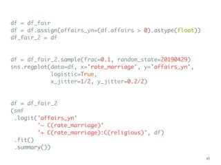
![More Estimations
➤ MLE, Maximum
Likelihood Estimation.
← Usually find by
numerical methods.
➤ TSLS, Two-Stage Least
Squares.
➤ y ← (x ← z)
➤ Handle the endogeneity:
E[ε|X] ≠ 0.
62](https://image.slidesharecdn.com/statisticalregressionwithpython-190511114627/75/Statistical-Regression-With-Python-62-2048.jpg)
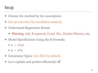
![Logit Model
➤ The coef is log-odds.
➤ Use exp(x)/(exp(x)+1) to
transform back to probability:
➤ 0.6931 → 67%
➤ ″ - 1.6664 → 27%
➤ ″ - 1.3503 → 9%
Or:
➤ .predict(dict(
rate_marriage=[1, 5, 5],
religious=[1, 1, 4]))
64](https://image.slidesharecdn.com/statisticalregressionwithpython-190511114627/75/Statistical-Regression-With-Python-64-2048.jpg)

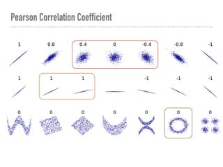
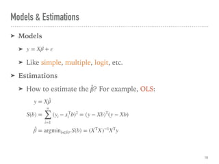
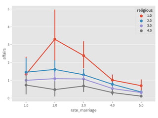
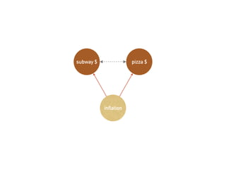
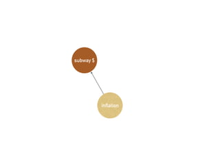
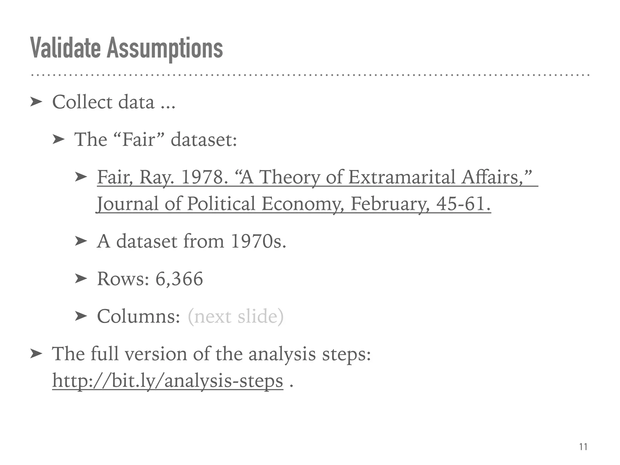
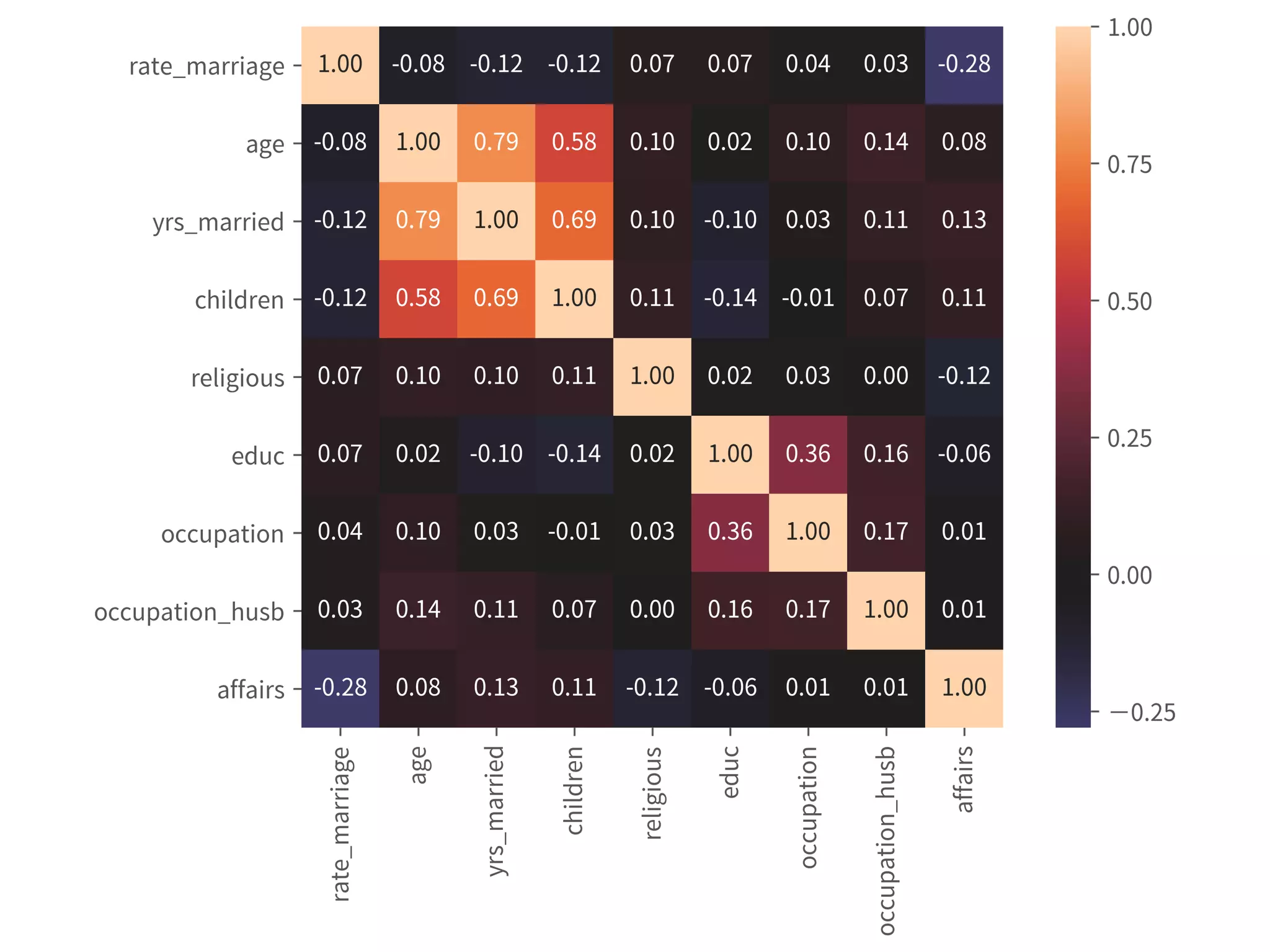
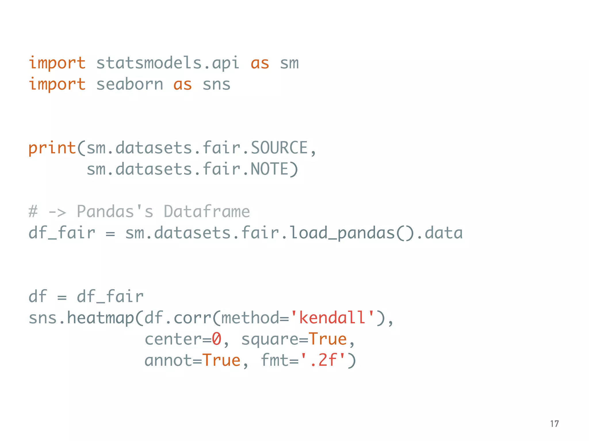
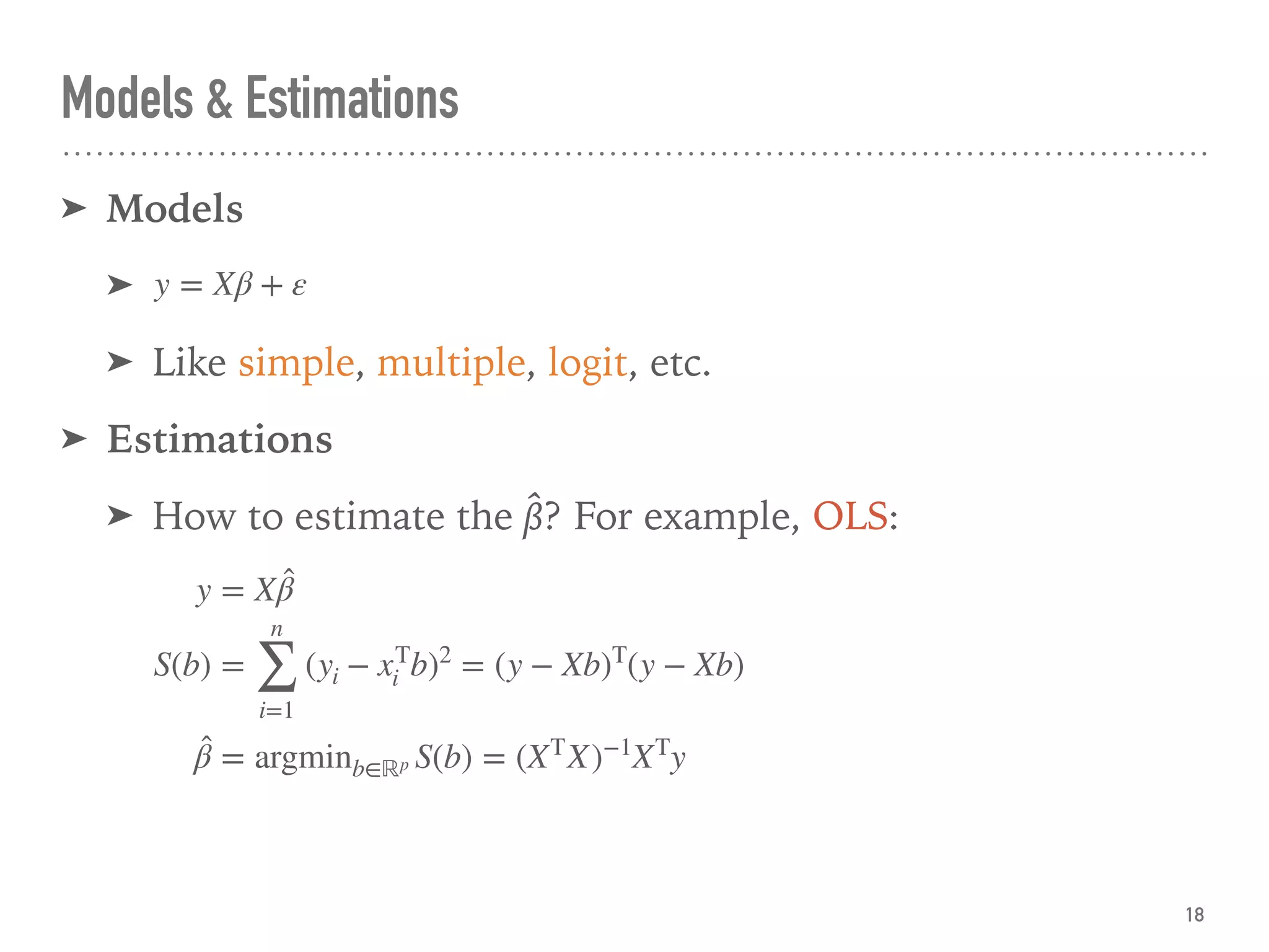
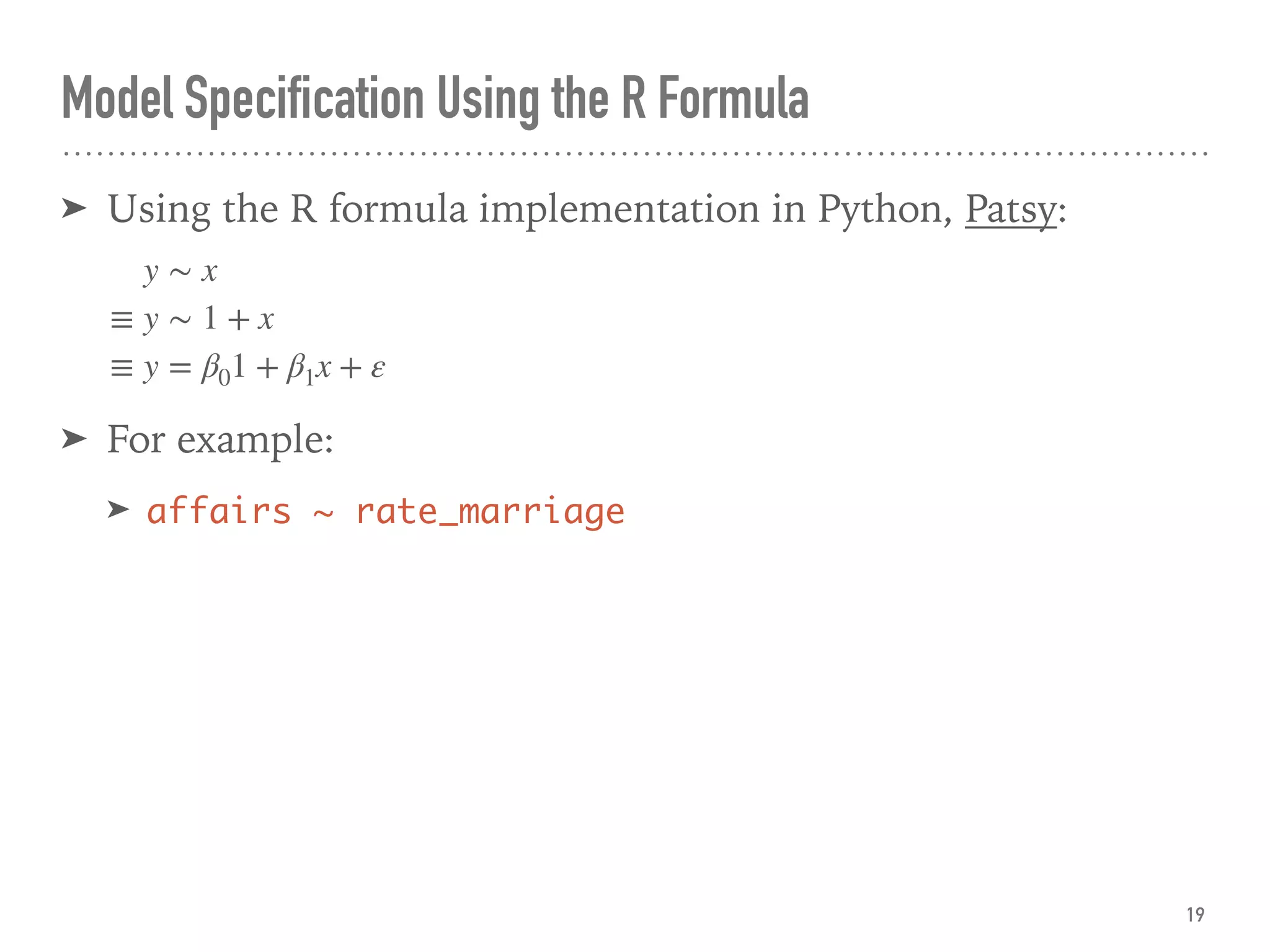
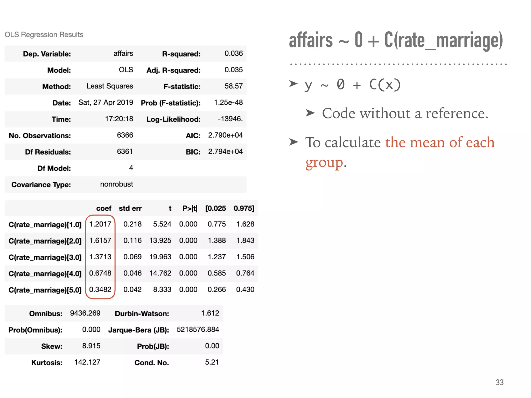
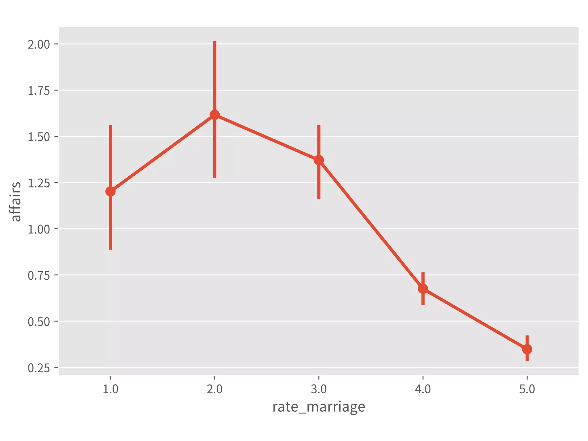
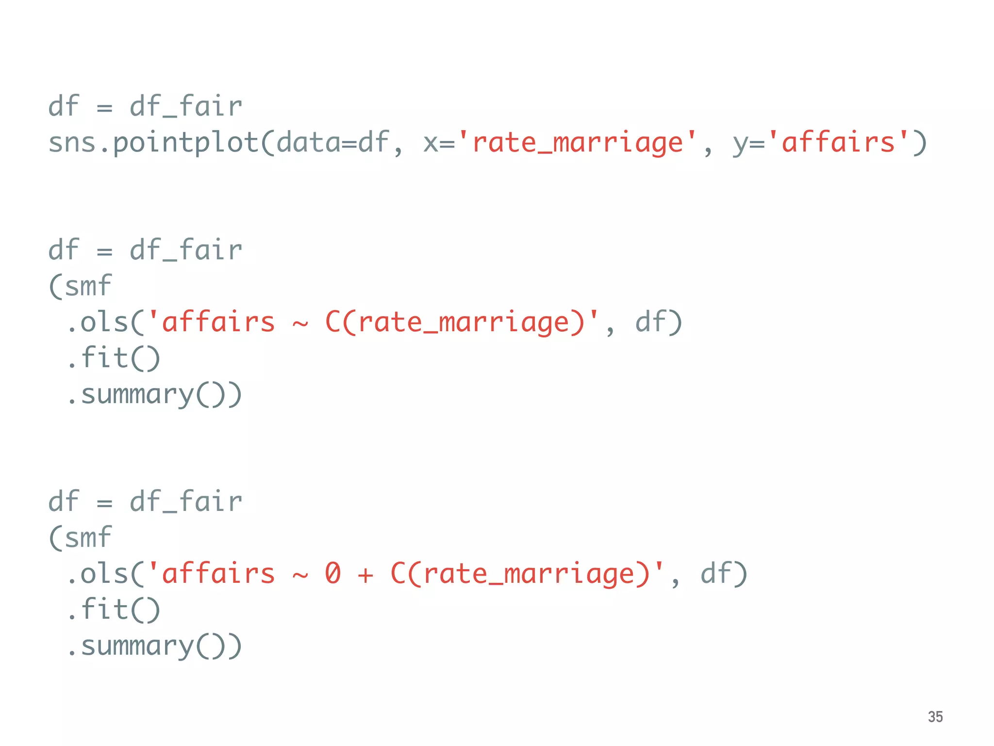
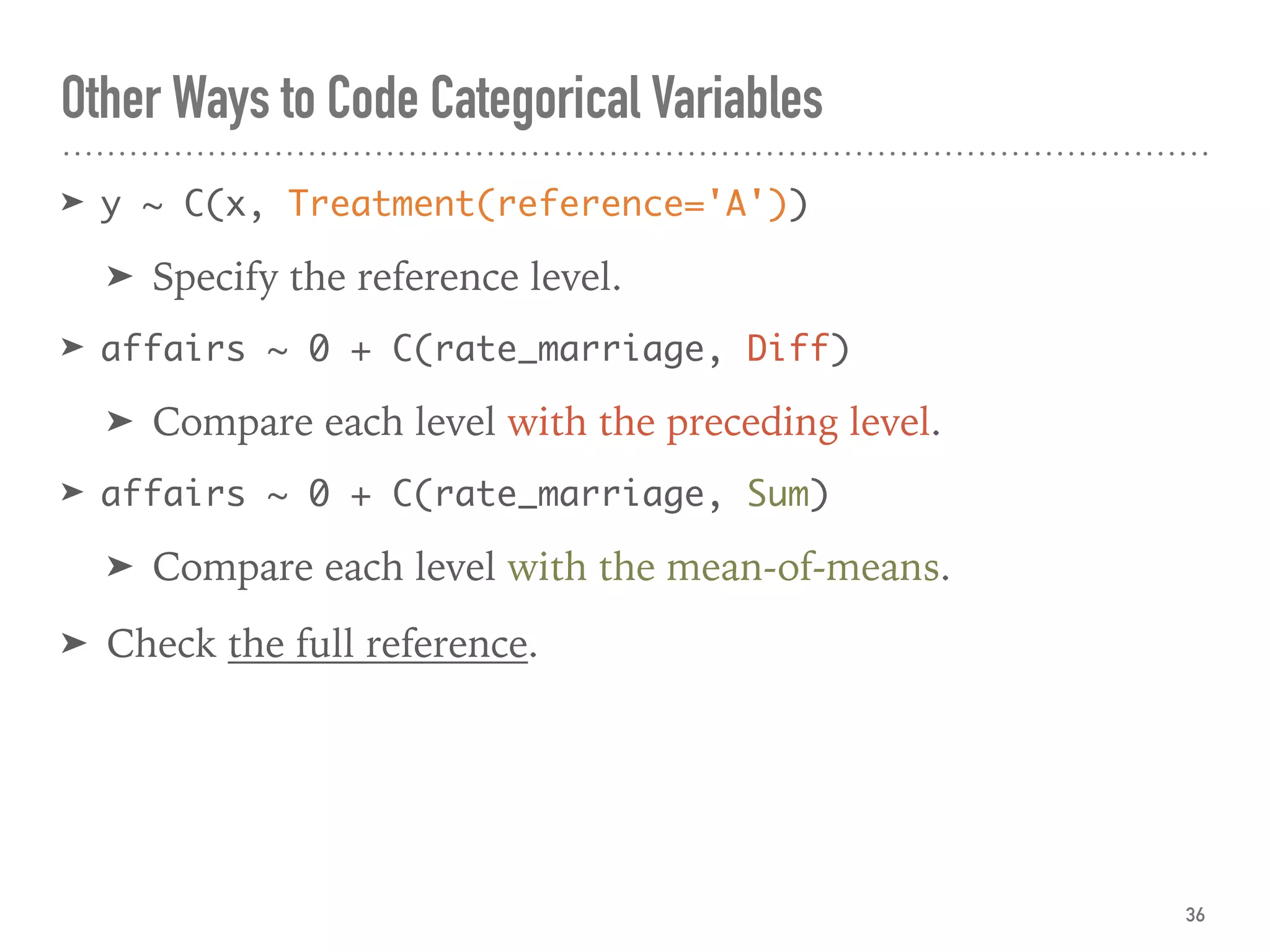
This document provides an overview of statistical regression analysis with Python. It discusses defining assumptions, validating assumptions with a dataset on extramarital affairs, performing correlation analysis, estimating models using ordinary least squares, understanding regression results including interaction effects, handling categorical variables, and addressing outliers. Modeling techniques covered include linear, logistic, and quantile regression as well as robust linear regression.


![Agentic Systems and Compliance - A brief intro [1.2]](https://cdn.slidesharecdn.com/ss_thumbnails/agenticsystemsandcompliace-1-251018025303-958a42ec-thumbnail.jpg?width=600ounds&width=560&fit=bounds)


![RTP_AR_Basic_Learners' Workbook_KS2 [FOR REPRODUCTION] (1).pdf](https://cdn.slidesharecdn.com/ss_thumbnails/rtparbasiclearnersworkbookks2forreproduction1-251016024943-e51a16ac-thumbnail.jpg?width=600ounds&width=560&fit=bounds)