Naive Bayes ClassifierAlgorithm
Naive Bayes algorithm is a supervised learning algorithm,
which is based on Bayes theorem and used for solving
classification problems.
It is mainly used in text classification that includes a high-
dimensional training dataset.
Naïve Bayes Classifier is one of the simple and most effective
Classification algorithms which helps in building the fast
machine learning models that can make quick predictions.
It is a probabilistic classifier, which means it predicts on the
basis of the probability of an object.
2.
Why is itcalled Naive Bayes?
•
The Naïve Bayes algorithm is comprised of two words Naïve and Bayes, Which
can be described as:
Naive: It is called Naïve because it assumes that the occurrence of a
certain feature is independent of the occurrence of other features. Such
as if the fruit is identified on the bases of color, shape, and taste, then red,
spherical, and sweet fruit is recognized as an apple. Hence each feature
individually contributes to identify that it is an apple without depending on
each other.
Bayes: It is called Bayes because it depends on the principle of Bayes'
Theorem.
3.
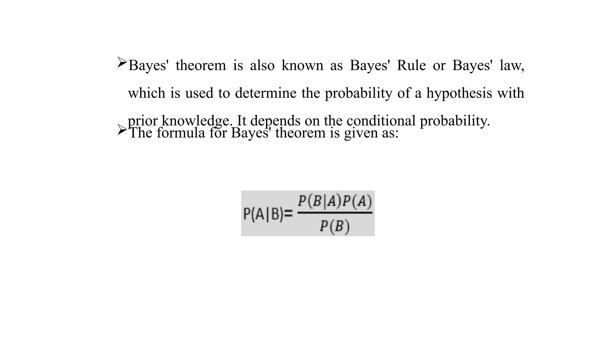
Bayes' theorem isalso known as Bayes' Rule or Bayes' law,
which is used to determine the probability of a hypothesis with
prior knowledge. It depends on the conditional probability.
The formula for Bayes' theorem is given as:
4.
P(A|B) is Posteriorprobability: Probability of hypothesis A
on the observed event B.
P(B|A) is Likelihood probability: Probability of the
evidence given that the probability of a hypothesis is
true.
P(A) is Prior Probability: Probability of hypothesis
before observing the evidence.
P(B) is Marginal Probability: Probability of
Evidence.
•
5.
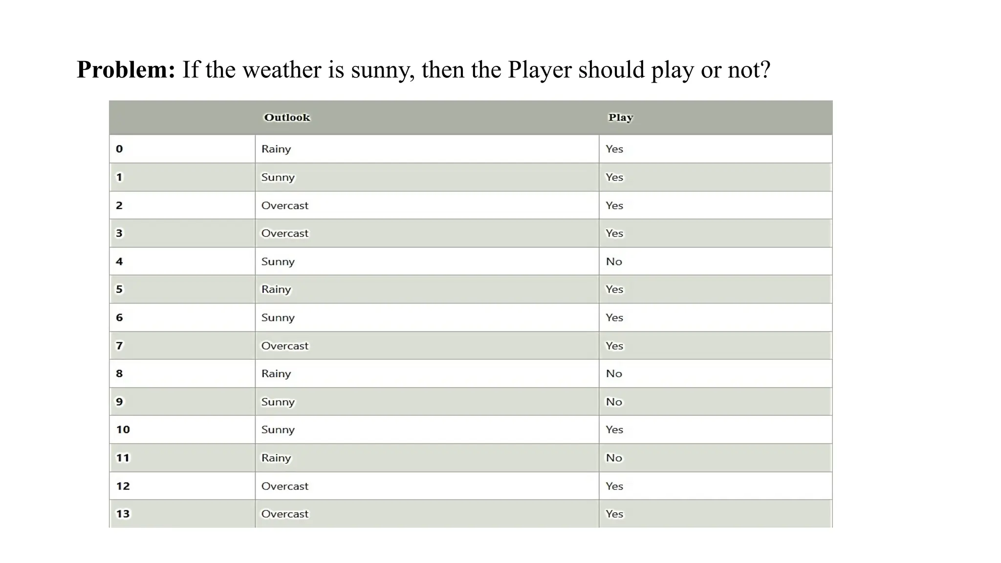
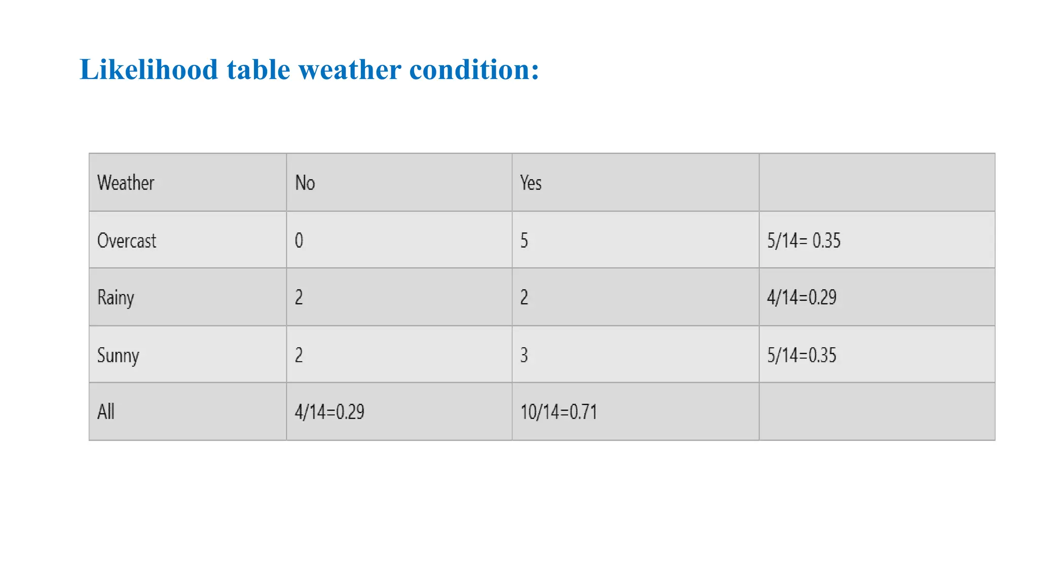
Problem: If theweather is sunny, then the Player should play or not?
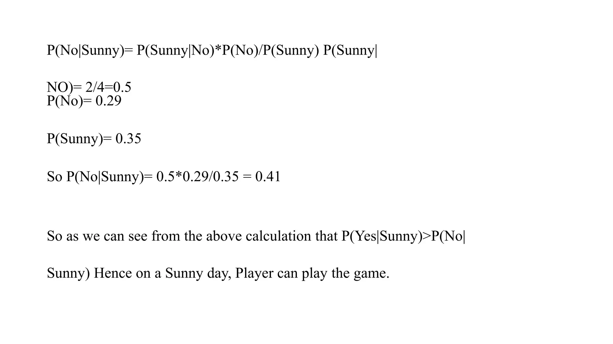
P(No|Sunny)= P(Sunny|No)*P(No)/P(Sunny) P(Sunny|
NO)=2/4=0.5
P(No)= 0.29
P(Sunny)= 0.35
So P(No|Sunny)= 0.5*0.29/0.35 = 0.41
So as we can see from the above calculation that P(Yes|Sunny)>P(No|
Sunny) Hence on a Sunny day, Player can play the game.
9.
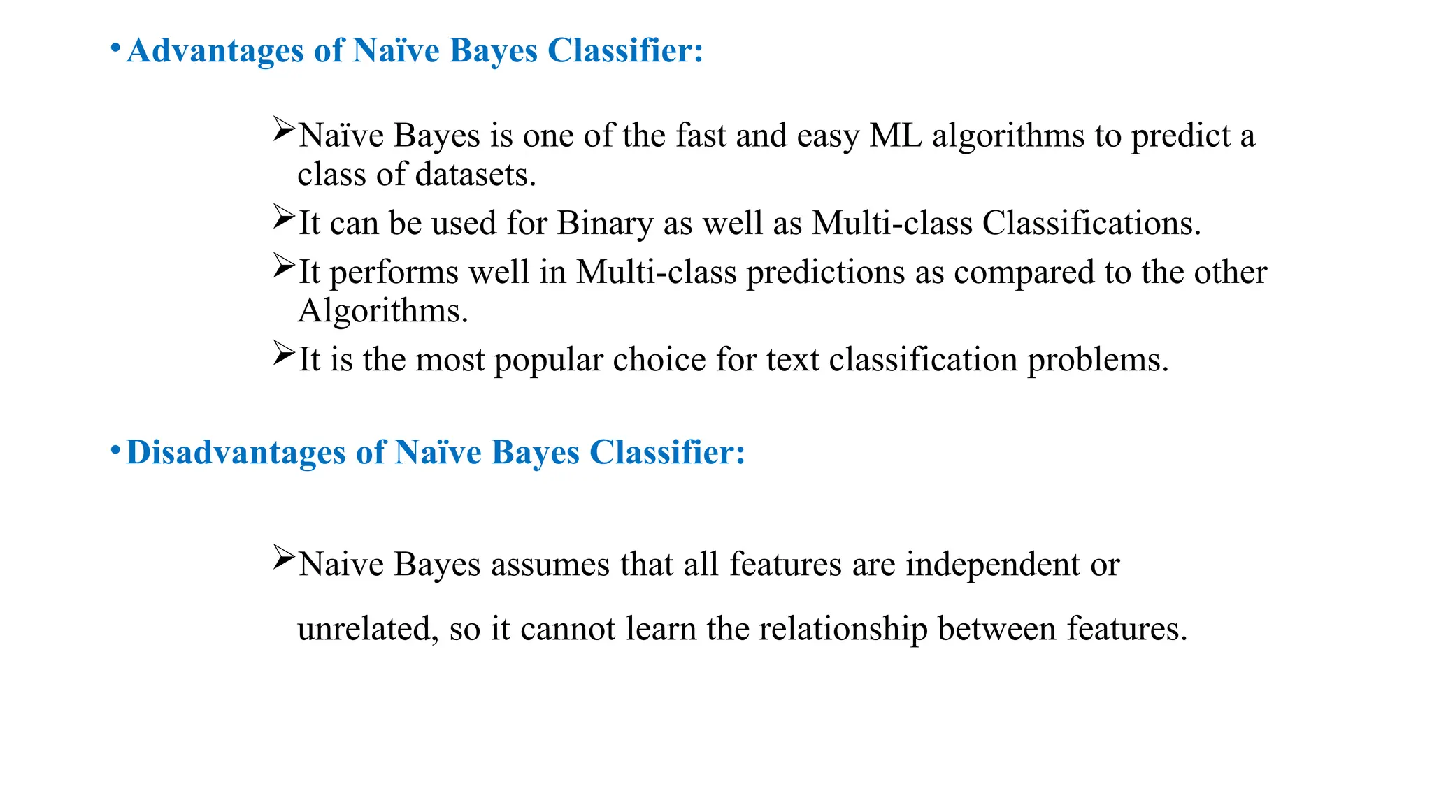
•Advantages of NaïveBayes Classifier:
Naïve Bayes is one of the fast and easy ML algorithms to predict a
class of datasets.
It can be used for Binary as well as Multi-class Classifications.
It performs well in Multi-class predictions as compared to the other
Algorithms.
It is the most popular choice for text classification problems.
•Disadvantages of Naïve Bayes Classifier:
Naive Bayes assumes that all features are independent or
unrelated, so it cannot learn the relationship between features.
10.
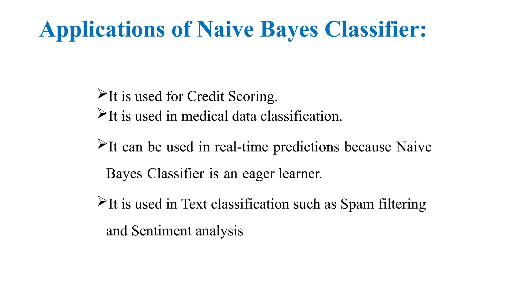
Applications of NaiveBayes Classifier:
It is used for Credit Scoring.
It is used in medical data classification.
It can be used in real-time predictions because Naive
Bayes Classifier is an eager learner.
It is used in Text classification such as Spam filtering
and Sentiment analysis
11.
SUPPORT VECTOR MACHINE
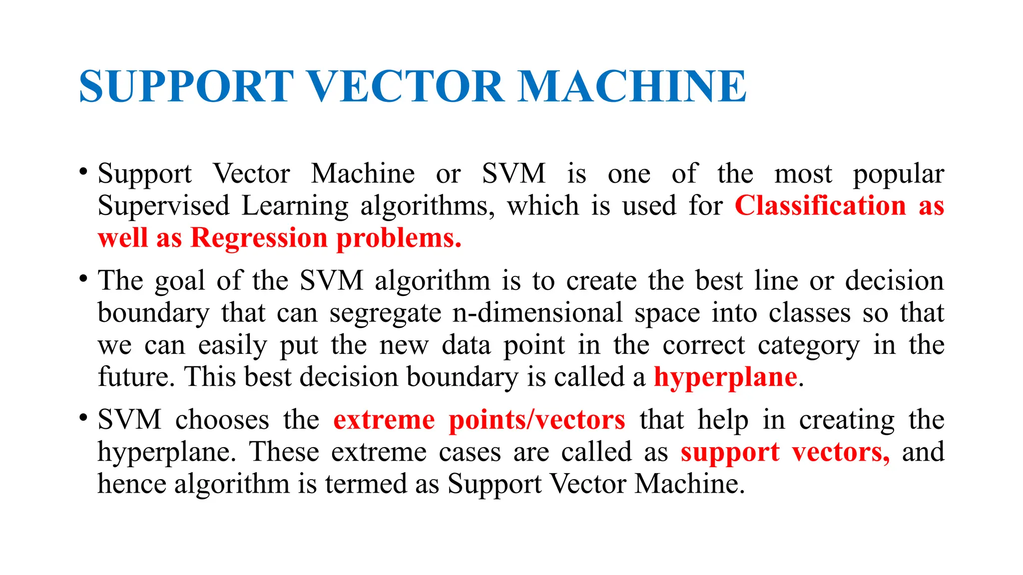
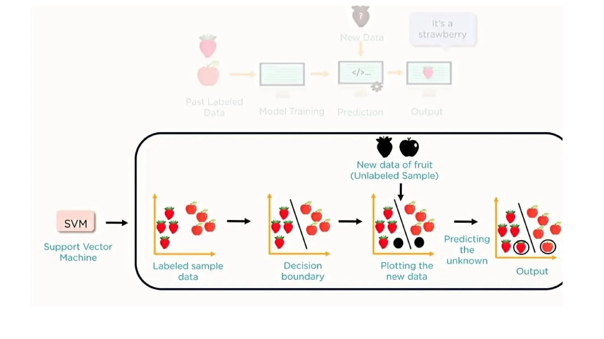
•Support Vector Machine or SVM is one of the most popular
Supervised Learning algorithms, which is used for Classification as
well as Regression problems.
• The goal of the SVM algorithm is to create the best line or decision
boundary that can segregate n-dimensional space into classes so that
we can easily put the new data point in the correct category in the
future. This best decision boundary is called a hyperplane.
• SVM chooses the extreme points/vectors that help in creating the
hyperplane. These extreme cases are called as support vectors, and
hence algorithm is termed as Support Vector Machine.
14.
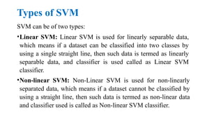
Types of SVM
SVMcan be of two types:
•Linear SVM: Linear SVM is used for linearly separable data,
which means if a dataset can be classified into two classes by
using a single straight line, then such data is termed as linearly
separable data, and classifier is used called as Linear SVM
classifier.
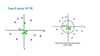
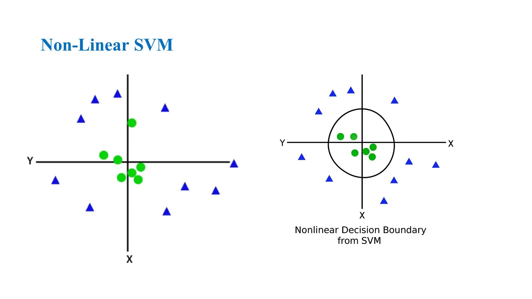
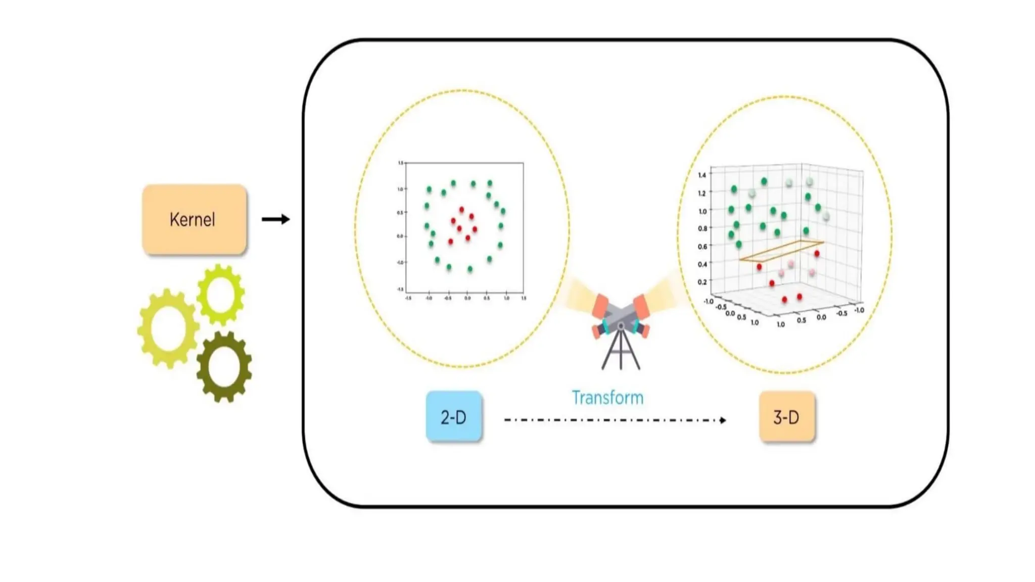
•Non-linear SVM: Non-Linear SVM is used for non-linearly
separated data, which means if a dataset cannot be classified by
using a straight line, then such data is termed as non-linear data
and classifier used is called as Non-linear SVM classifier.
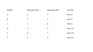
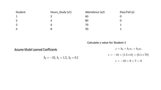
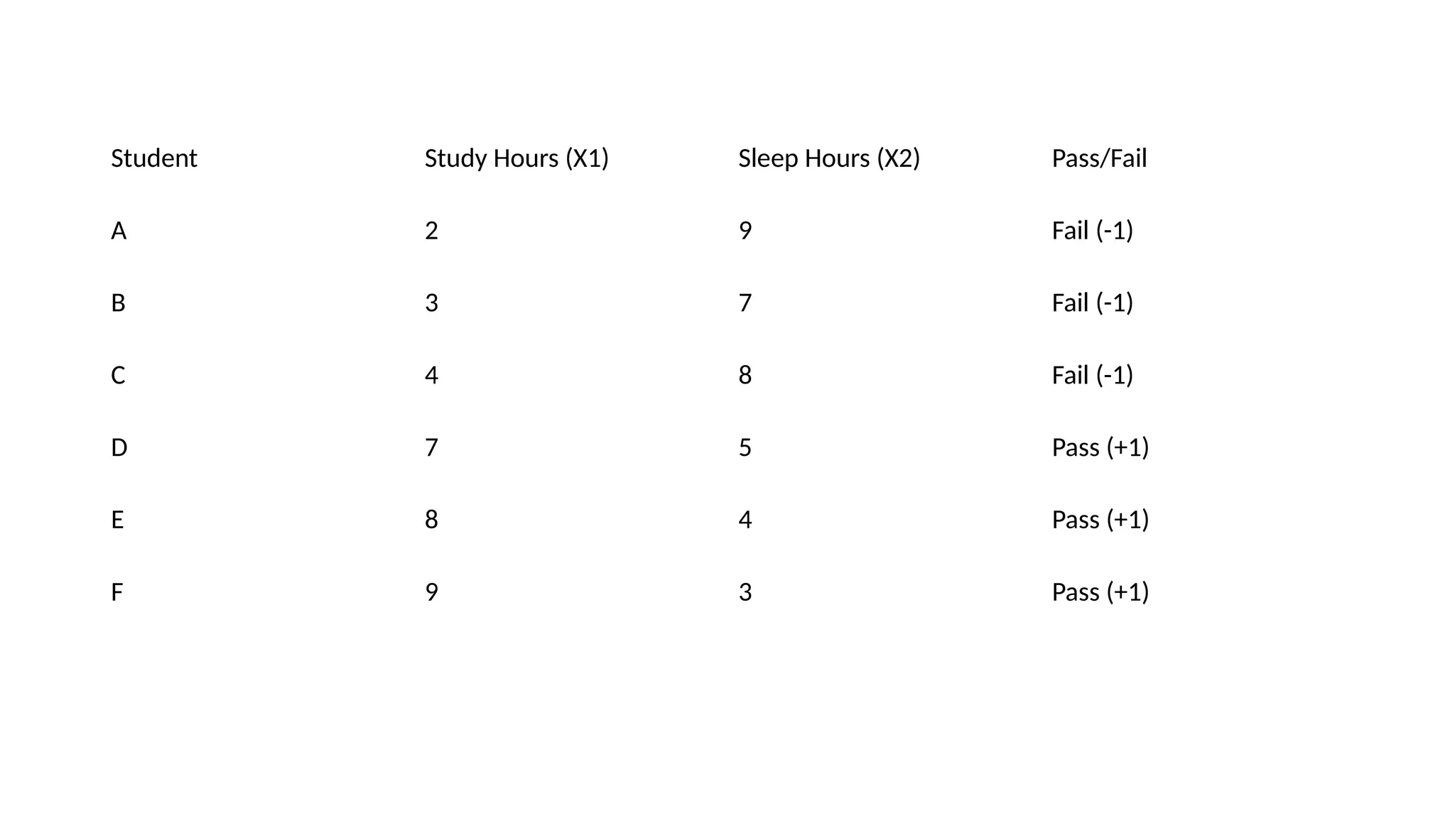
Student Study Hours(X1) Sleep Hours (X2) Pass/Fail
A 2 9 Fail (-1)
B 3 7 Fail (-1)
C 4 8 Fail (-1)
D 7 5 Pass (+1)
E 8 4 Pass (+1)
F 9 3 Pass (+1)
18.
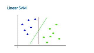
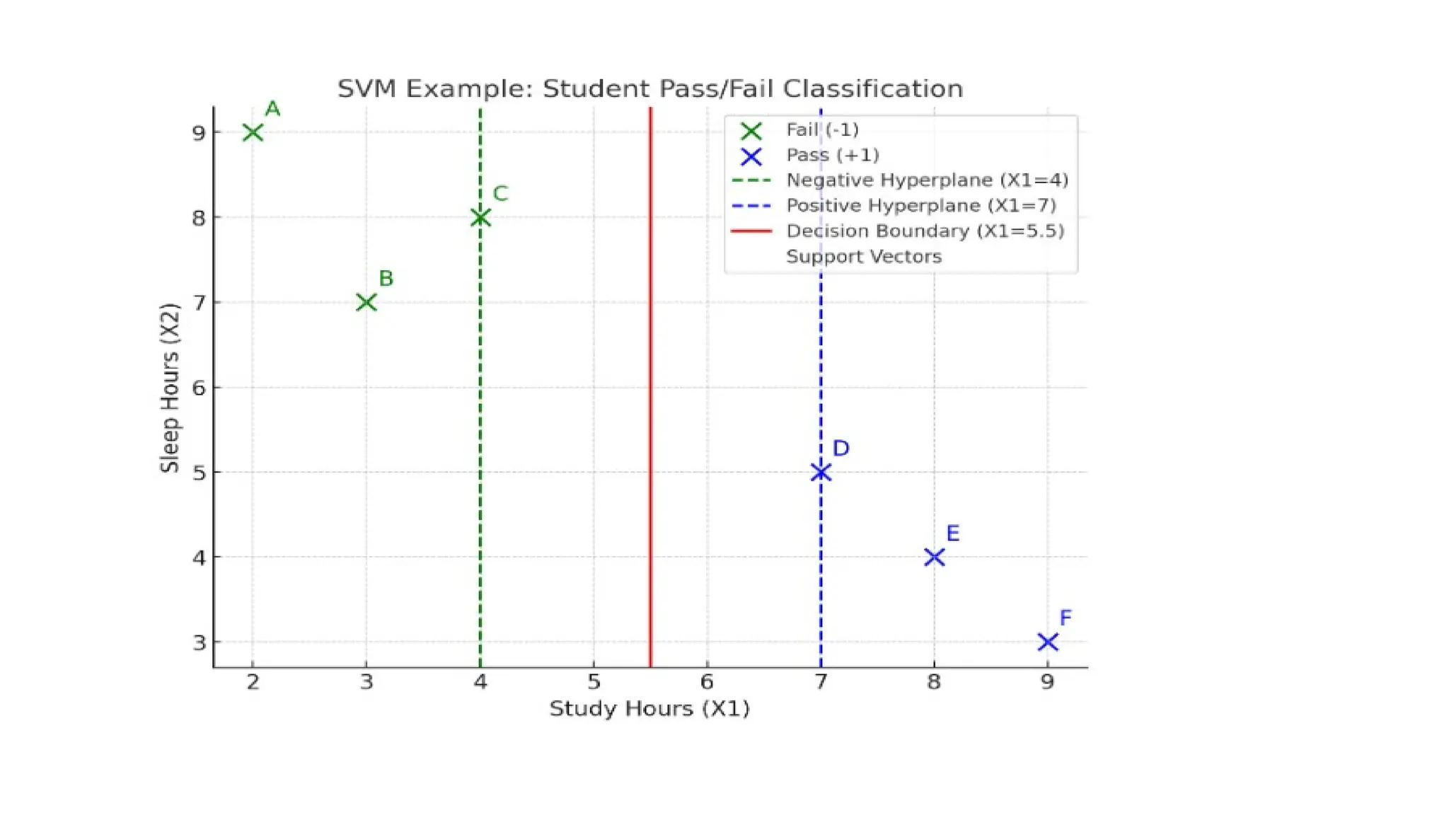
Step 1: Plotthe Points
• X-axis → Study Hours (X1)
• Y-axis → Sleep Hours (X2)
Step 2: Identify the Separating Line (Hyperplane)
• We need a line that separates green points from blue points.
• Observing data:
• Fail students: Study hours ≤ 4
• Pass students: Study hours ≥ 7
A simple decision boundary is around X1 = 5.5 (vertical line).
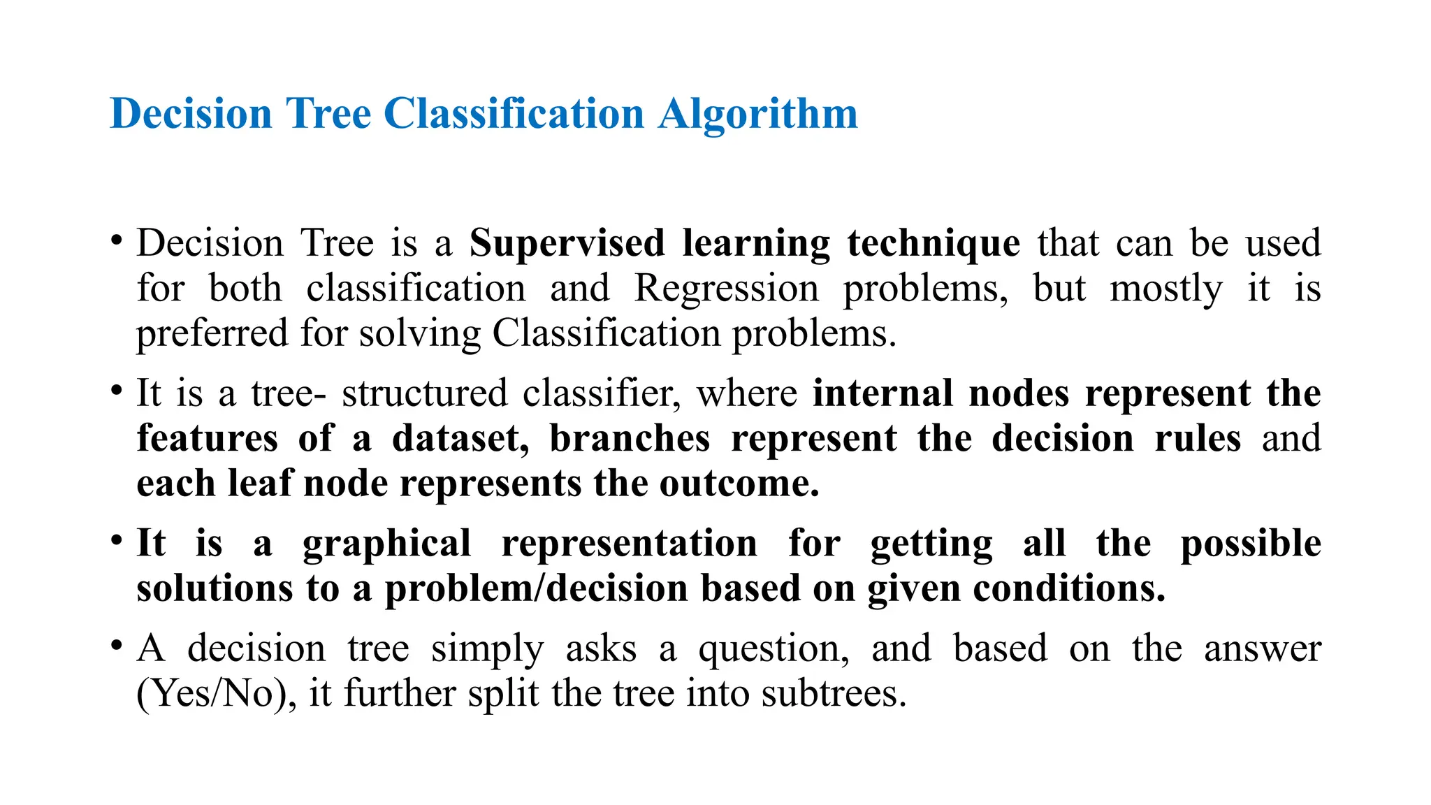
Decision Tree ClassificationAlgorithm
• Decision Tree is a Supervised learning technique that can be used
for both classification and Regression problems, but mostly it is
preferred for solving Classification problems.
• It is a tree- structured classifier, where internal nodes represent the
features of a dataset, branches represent the decision rules and
each leaf node represents the outcome.
• It is a graphical representation for getting all the possible
solutions to a problem/decision based on given conditions.
• A decision tree simply asks a question, and based on the answer
(Yes/No), it further split the tree into subtrees.
26.
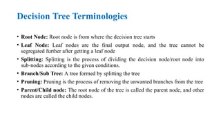
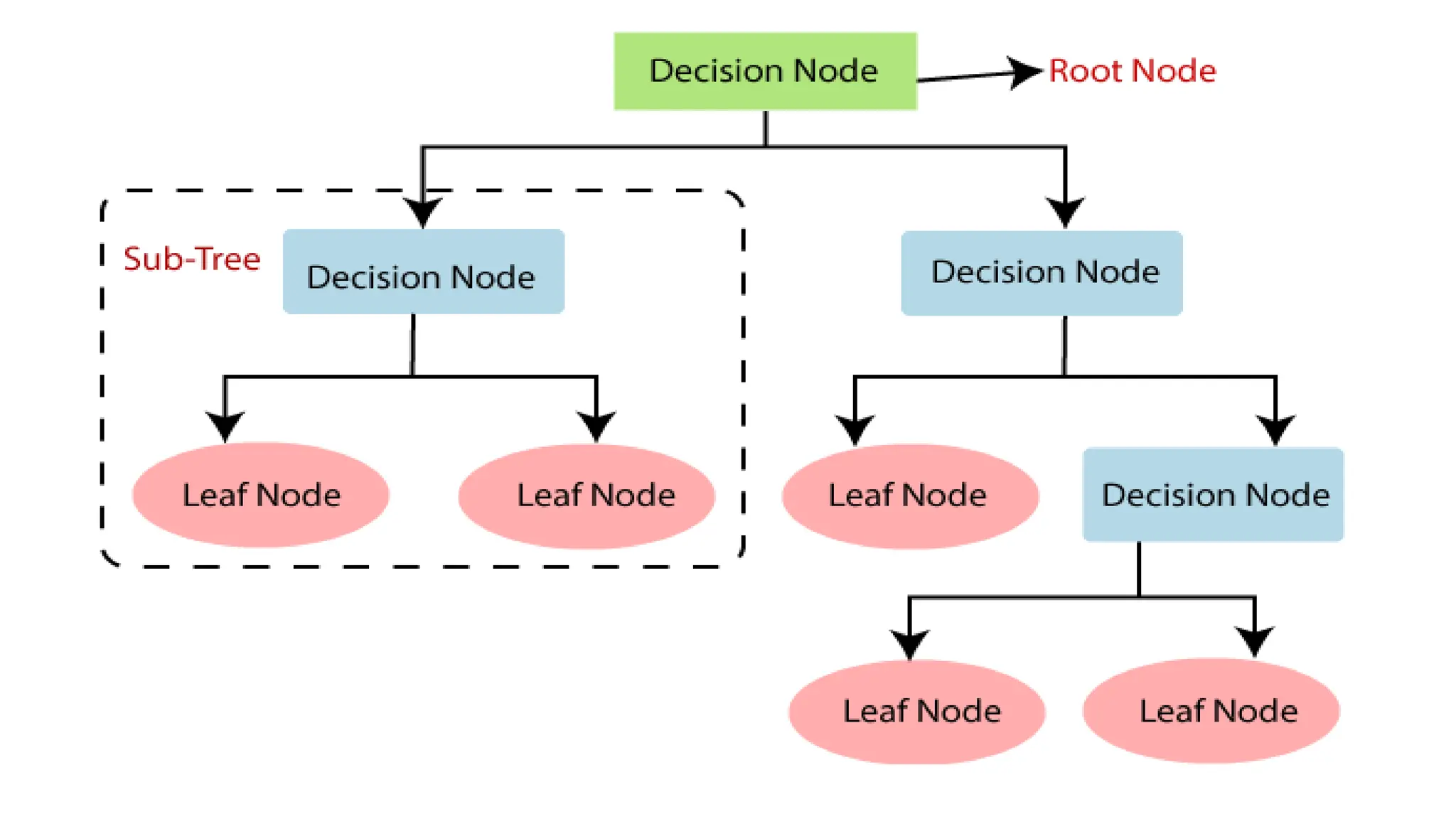
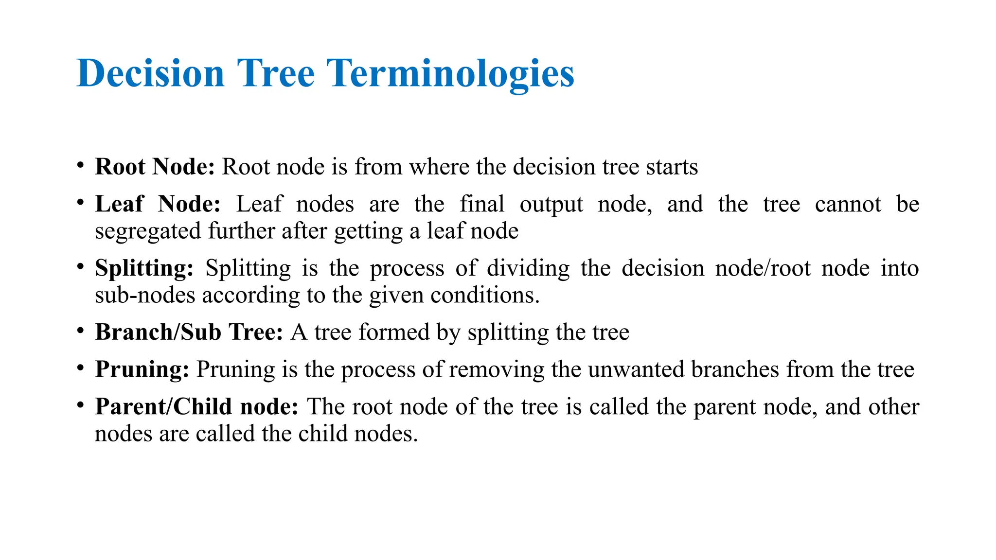
Decision Tree Terminologies
•Root Node: Root node is from where the decision tree starts
• Leaf Node: Leaf nodes are the final output node, and the tree cannot be
segregated further after getting a leaf node
• Splitting: Splitting is the process of dividing the decision node/root node into
sub-nodes according to the given conditions.
• Branch/Sub Tree: A tree formed by splitting the tree
• Pruning: Pruning is the process of removing the unwanted branches from the tree
• Parent/Child node: The root node of the tree is called the parent node, and other
nodes are called the child nodes.
27.
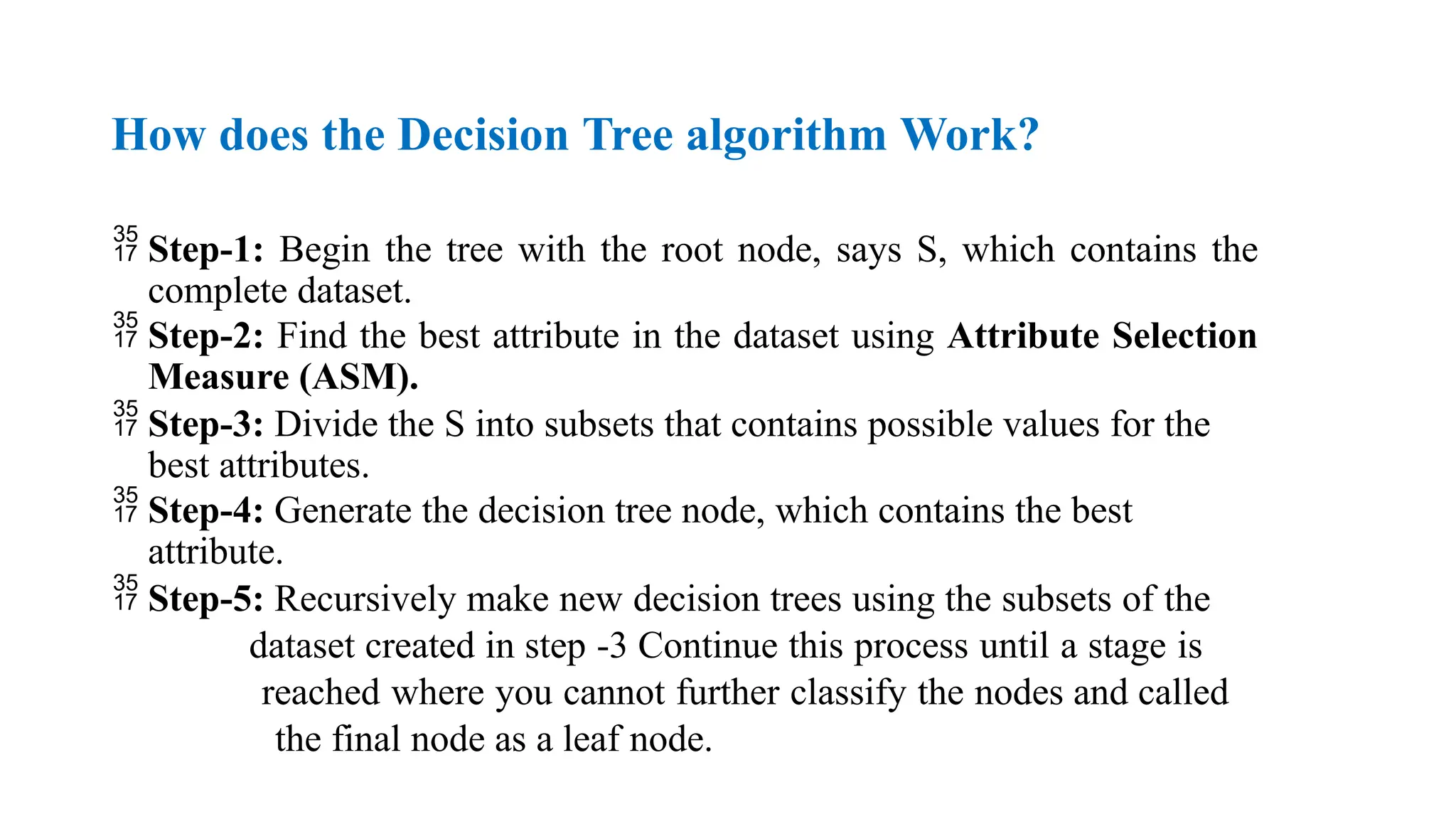
How does theDecision Tree algorithm Work?
Step-1: Begin the tree with the root node, says S, which contains the
complete dataset.
Step-2: Find the best attribute in the dataset using Attribute Selection
Measure (ASM).
Step-3: Divide the S into subsets that contains possible values for the
best attributes.
Step-4: Generate the decision tree node, which contains the best
attribute.
Step-5: Recursively make new decision trees using the subsets of the
dataset created in step -3 Continue this process until a stage is
reached where you cannot further classify the nodes and called
the final node as a leaf node.
29.
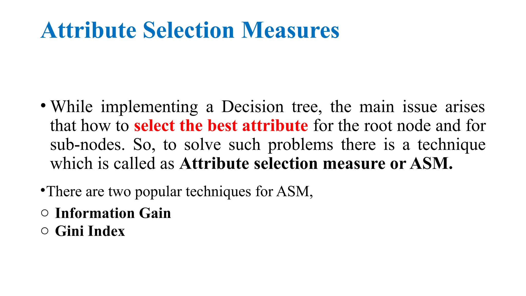
Attribute Selection Measures
•While implementing a Decision tree, the main issue arises
that how to select the best attribute for the root node and for
sub-nodes. So, to solve such problems there is a technique
which is called as Attribute selection measure or ASM.
•There are two popular techniques for ASM,
o Information Gain
o Gini Index
30.
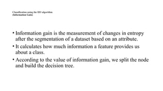
Classification using theID3 algorithm
(Information Gain)
• Information gain is the measurement of changes in entropy
after the segmentation of a dataset based on an attribute.
• It calculates how much information a feature provides us
about a class.
• According to the value of information gain, we split the node
and build the decision tree.
32.
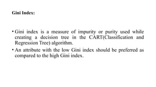
Gini Index:
• Giniindex is a measure of impurity or purity used while
creating a decision tree in the CART(Classification and
Regression Tree) algorithm.
• An attribute with the low Gini index should be preferred as
compared to the high Gini index.
33.
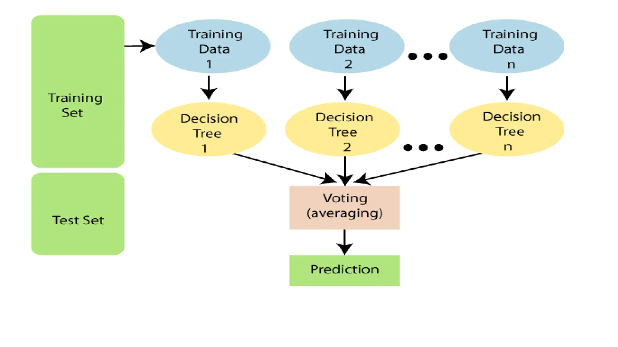
RANDOM FOREST ALGORITHM
•Random Forest is a popular machine learning algorithm that belongs
to the supervised learning technique.
• It can be used for both Classification and Regression problems in ML.
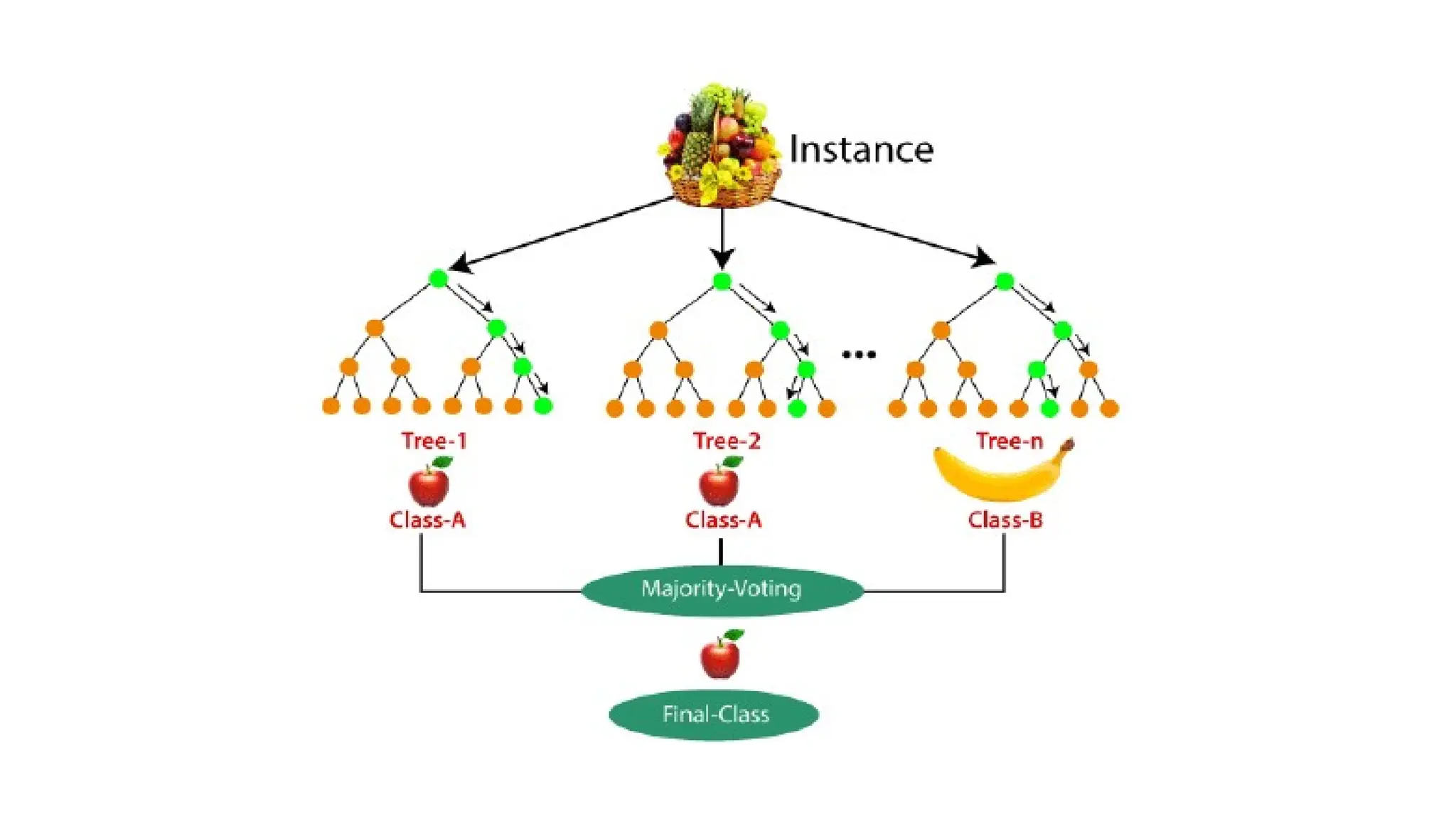
• "Random Forest is a classifier that contains a number of decision
trees on various subsets of the given dataset and takes the average to
improve the predictive accuracy of that dataset.“
• It is based on the concept of ensemble learning, which is a process of
combining multiple classifiers to solve a complex problem and to
improve the performance of the model.
35.
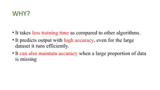
WHY?
• It takesless training time as compared to other algorithms.
• It predicts output with high accuracy, even for the large
dataset it runs efficiently.
• It can also maintain accuracy when a large proportion of data
is missing
36.
THE WORKING PROCESS
•Step-1: Select random K data points from the training set.
• Step-2: Build the decision trees associated with the selected data
points (Subsets).
• Step-3: Choose the number N for decision trees that you want to
build.
• Step-4: Repeat Step 1 & 2.
• Step-5: For new data points, find the predictions of each decision tree,
and assign the new data points to the category that wins the majority
votes.
38.
Advantages of RandomForest
• Random Forest is capable of performing both Classification
and Regression tasks.
• It is capable of handling large datasets with high
dimensionality.
• It enhances the accuracy of the model and prevents the
overfitting issue.
39.
LOGISTIC REGRESSION INMACHINE LEARNING
• Logistic regression is one of the most popular Machine Learning
algorithms, which comes under the Supervised Learning technique. It
is used for predicting the categorical dependent variable using a given
set of independent variables.
• Logistic regression predicts the output of a categorical dependent
variable. Therefore the outcome must be a categorical or discrete
value. It can be either Yes or No, 0 or 1, true or False, etc.
• In Logistic regression, instead of fitting a regression line, we fit an "S"
shaped logistic function, which predicts two maximum values (0 or 1).
41.
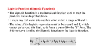
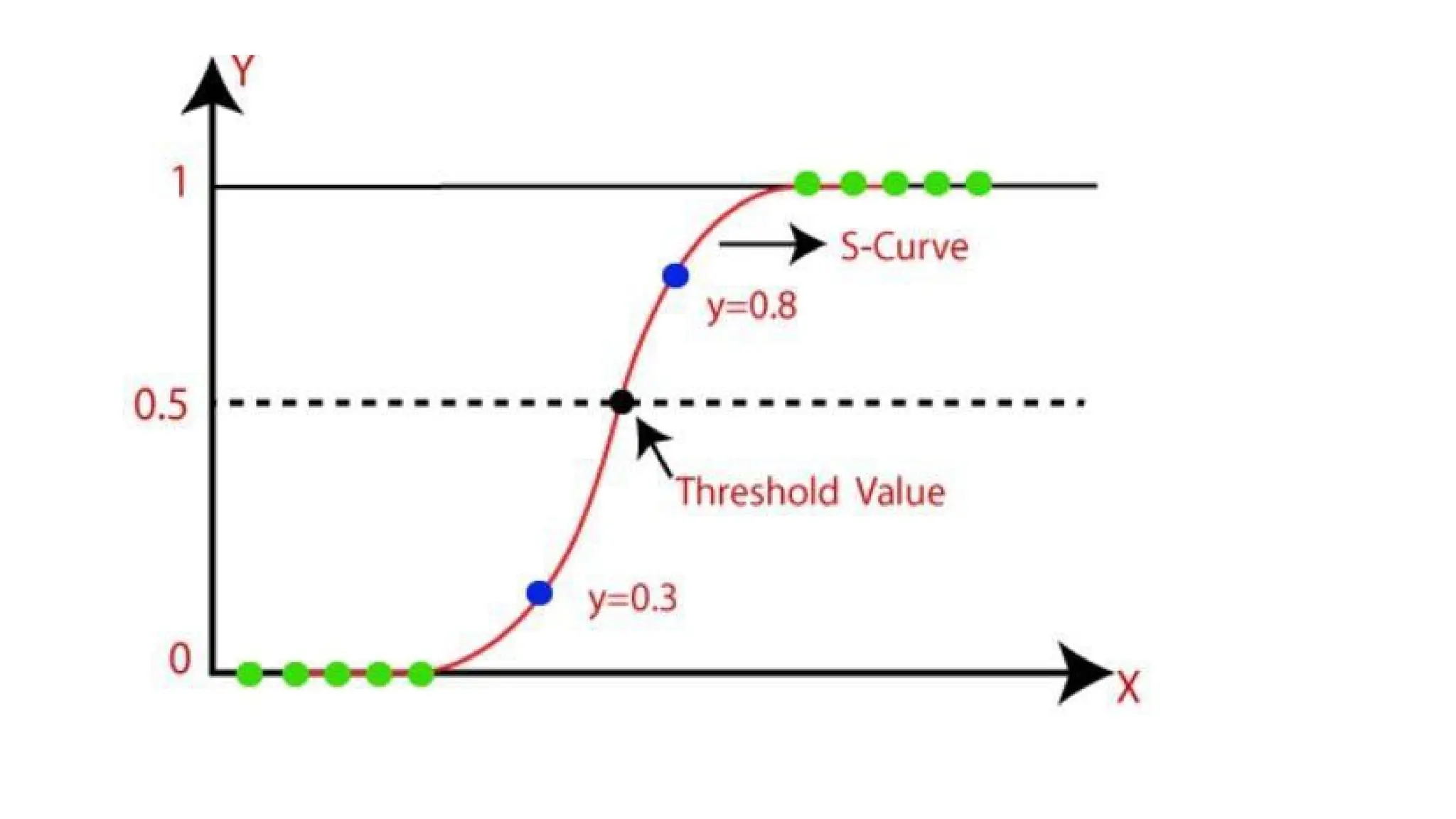
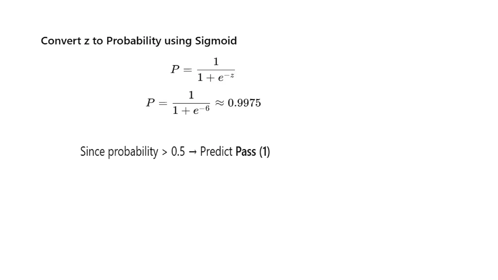
Logistic Function (SigmoidFunction):
• The sigmoid function is a mathematical function used to map the
predicted values to probabilities.
• It maps any real value into another value within a range of 0 and 1.
• The value of the logistic regression must be between 0 and 1, which
cannot go beyond this limit, so it forms a curve like the "S" form. The
S-form curve is called the Sigmoid function or the logistic function.
42.
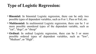
Type of LogisticRegression:
• Binomial: In binomial Logistic regression, there can be only two
possible types of dependent variables, such as 0 or 1, Pass or Fail, etc.
• Multinomial: In multinomial Logistic regression, there can be 3 or
more possible unordered types of the dependent variable, such as
"cat", "dogs", or "sheep"
• Ordinal: In ordinal Logistic regression, there can be 3 or more
possible ordered types of dependent variables, such as "low",
"Medium", or "High".
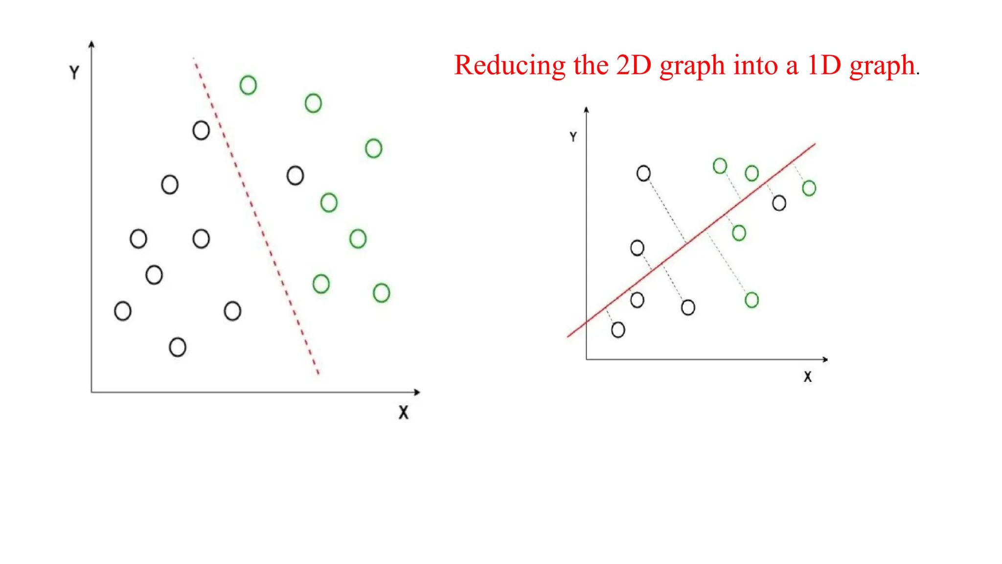
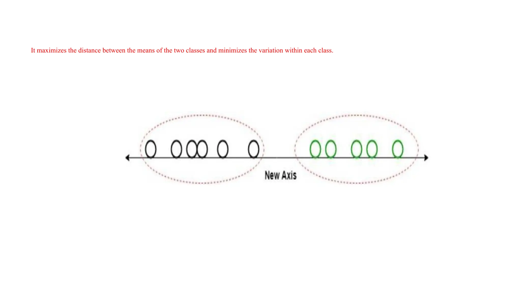
Discriminant Functions
• DiscriminantFunction Analysis is a dimensionality reduction technique that is
commonly used for supervised classification problems.
• For example, we have two classes, and we need to separate them efficiently.
Classes can have multiple features. Using only a single feature to classify them
may result in some overlapping as shown in the below figure. So, we will keep on
increasing the number of features for proper classification.
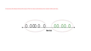
It maximizes thedistance between the means of the two classes and minimizes the variation within each class.
48.
GRADIENT DESCENT INMACHINE LEARNING
• Gradient Descent is known as one of the most commonly used optimization
algorithms to train machine learning models by means of minimizing errors
between actual and expected results.
• In mathematical terminology, Optimization algorithm refers to the task of
minimizing/maximizing an objective function f(x) parameterized by x. Similarly,
in machine learning, optimization is the task of minimizing the cost function
parameterized by the model's parameters.
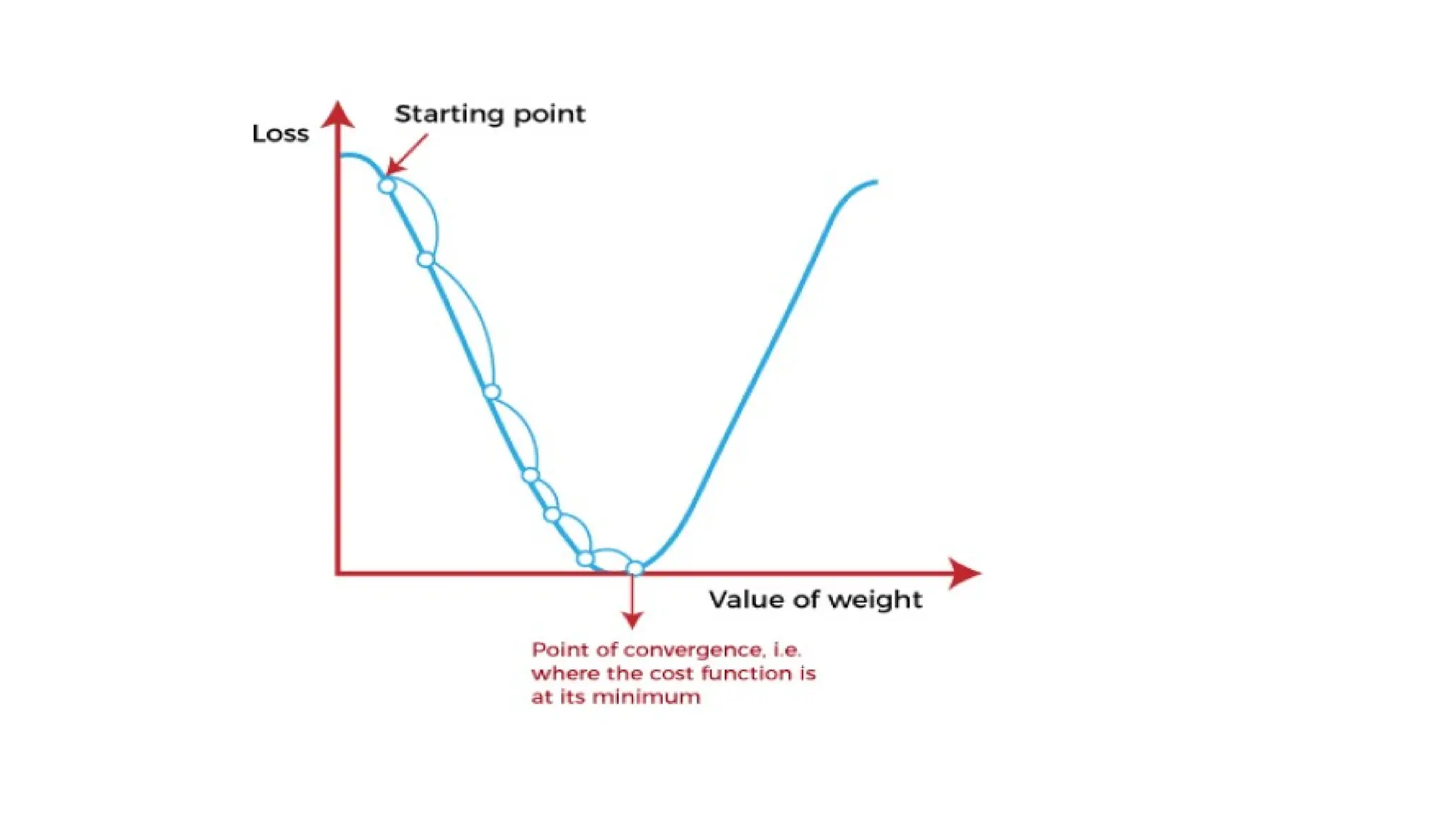
• “Gradient Descent is defined as one of the most commonly used iterative
optimization algorithms of machine learning to train the machine learning and
deep learning models. It helps in finding the local minimum of a function.”
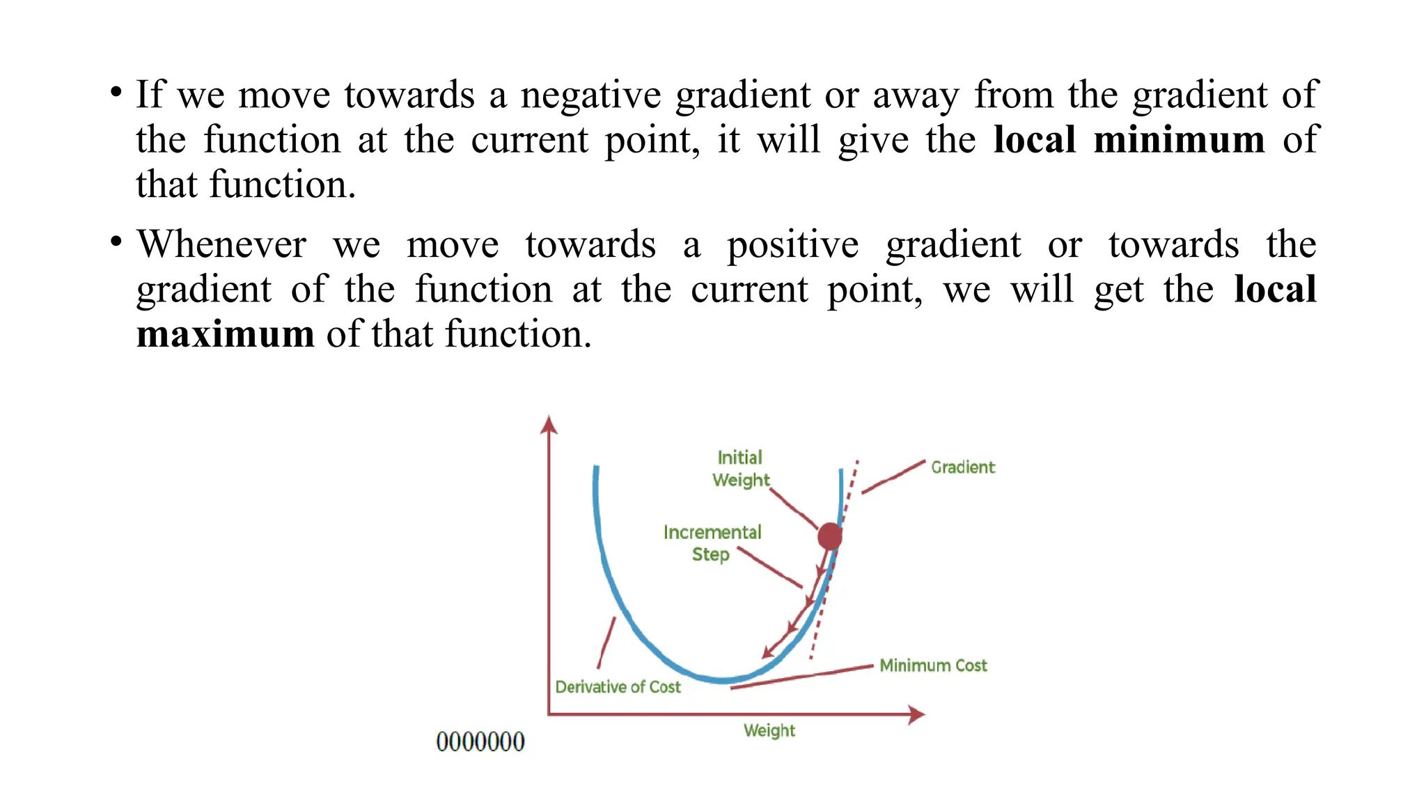
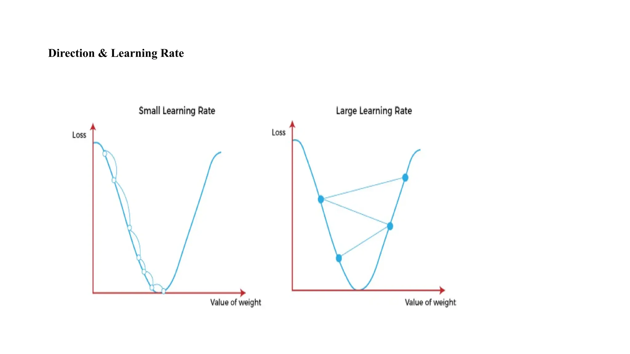
49.
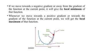
• If wemove towards a negative gradient or away from the gradient of
the function at the current point, it will give the local minimum of
that function.
• Whenever we move towards a positive gradient or towards the
gradient of the function at the current point, we will get the local
maximum of that function.
50.
Cost-function
The cost functionis defined as the measurement of
difference or error between actual values and expected
values at the current position
Types of GradientDescent
• Batch gradient descent,
• stochastic gradient descent, and
• mini-batch gradient descent
54.
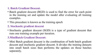
1. Batch GradientDescent:
• Batch gradient descent (BGD) is used to find the error for each point
in the training set and update the model after evaluating all training
examples.
• This procedure is known as the training epoch
2. Stochastic gradient descent
• Stochastic gradient descent (SGD) is a type of gradient descent that
runs one training example per iteration.
3.MiniBatch Gradient Descent:
• Mini Batch gradient descent is the combination of both batch gradient
descent and stochastic gradient descent. It divides the training datasets
into small batch sizes then performs the updates on those batches
separately.
55.
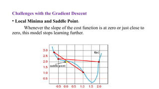
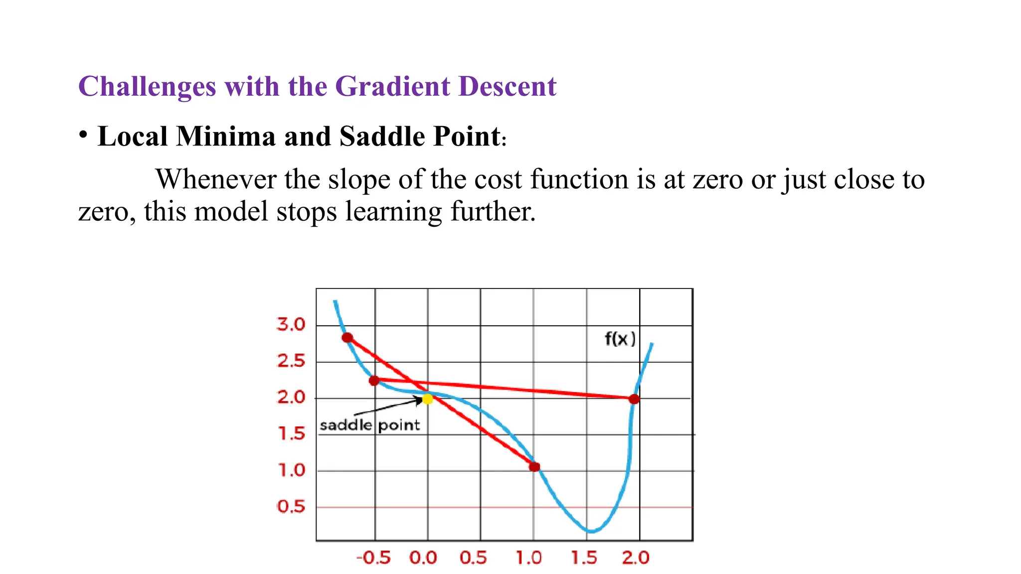
Challenges with theGradient Descent
• Local Minima and Saddle Point:
Whenever the slope of the cost function is at zero or just close to
zero, this model stops learning further.
56.
2.Vanishing and ExplodingGradient
Vanishing Gradients:
• Vanishing Gradient occurs when the gradient is smaller than expected.
Exploding Gradient:
• Exploding gradient is just opposite to the vanishing gradient as it
occurs when the Gradient is too large and creates a stable model.
Editor's Notes
#1 Naive Bayes – Concept Overview (Slide Style)
Type:
Supervised Learning Algorithm (Classification)
Based on:
Bayes Theorem (Probability)
Nature:
Probabilistic Classifier → Predicts using probability of each class
Goal:
ஒரு புதிய data point வந்தா, அது எந்த class-க்கு சேரும் என்பதை
probability calculation வைத்து predict பண்ணுது.
Real-Life Analogy:
Doctor checks symptoms → Calculates disease probability → Predicts Flu / Cold
#2 Example: Fruit Identification
Features to identify a fruit:
Color → Red
Shape → Spherical
Taste → Sweet
Naive Bayes assumes that:
The color being red does not depend on the shape being spherical.
The taste being sweet does not depend on the color being red.
#40 X‑Axis: Represents the linear input z=b0+b1x1+...z = b_0 + b_1x_1 + ...z=b0+b1x1+...
Y‑Axis: Represents the probability output of the sigmoid function (0 to 1)