Outline
Motivation
TechnicalSolution
Uninformed Search
Depth-First Search
Breadth-First Search
Informed Search
Best-First Search
Hill Climbing
A*
Illustration by a Larger Example
Extensions
Summary
3.
Motivation
One ofthe major goals of AI is to help humans in solving complex tasks
How can I fill my container with pallets?
Which is the shortest way from Milan to Innsbruck?
Which is the fastest way from Milan to Innsbruck?
How can I optimize the load of my freight to maximize my revenue?
How can I solve my Sudoku game?
What is the sequence of actions I should apply to win a game?
Sometimes finding a solution is not enough, you want the optimal solution
according to some “cost” criteria
All the example presented above involve looking for a plan
A plan that can be defined as the set of operations to be performed of an
initial state, to reach a final state that is considered the goal state
Thus we need efficient techniques to search for paths, or sequences of
actions, that can enable us to reach the goal state, i.e. to find a plan
Such techniques are commonly called Search Methods
4.
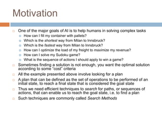
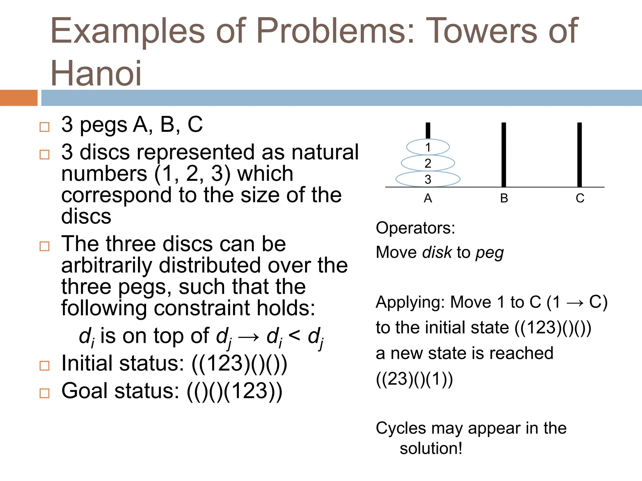
Examples of Problems:Towers of
Hanoi
3 pegs A, B, C
3 discs represented as natural
numbers (1, 2, 3) which
correspond to the size of the
discs
The three discs can be
arbitrarily distributed over the
three pegs, such that the
following constraint holds:
di is on top of dj → di < dj
Initial status: ((123)()())
Goal status: (()()(123))
3
2
1
A B C
Operators:
Move disk to peg
Applying: Move 1 to C (1 → C)
to the initial state ((123)()())
a new state is reached
((23)()(1))
Cycles may appear in the
solution!
5.
Examples of Problems:
Blocksworld
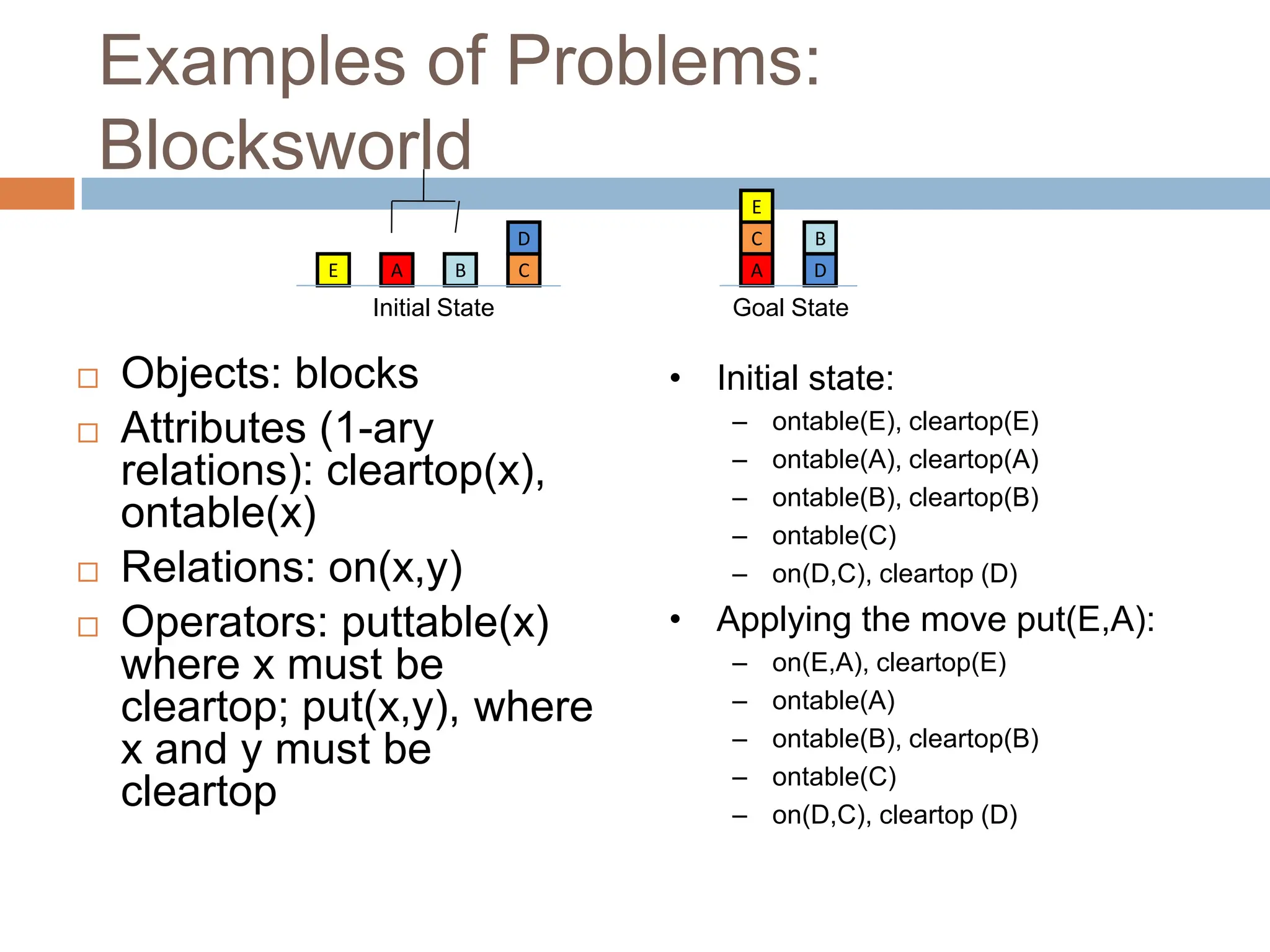
Objects: blocks
Attributes (1-ary
relations): cleartop(x),
ontable(x)
Relations: on(x,y)
Operators: puttable(x)
where x must be
cleartop; put(x,y), where
x and y must be
cleartop
E
A
B
C
D
Goal State
E A B C
D
Initial State
• Initial state:
– ontable(E), cleartop(E)
– ontable(A), cleartop(A)
– ontable(B), cleartop(B)
– ontable(C)
– on(D,C), cleartop (D)
• Applying the move put(E,A):
– on(E,A), cleartop(E)
– ontable(A)
– ontable(B), cleartop(B)
– ontable(C)
– on(D,C), cleartop (D)
Search Space Representation
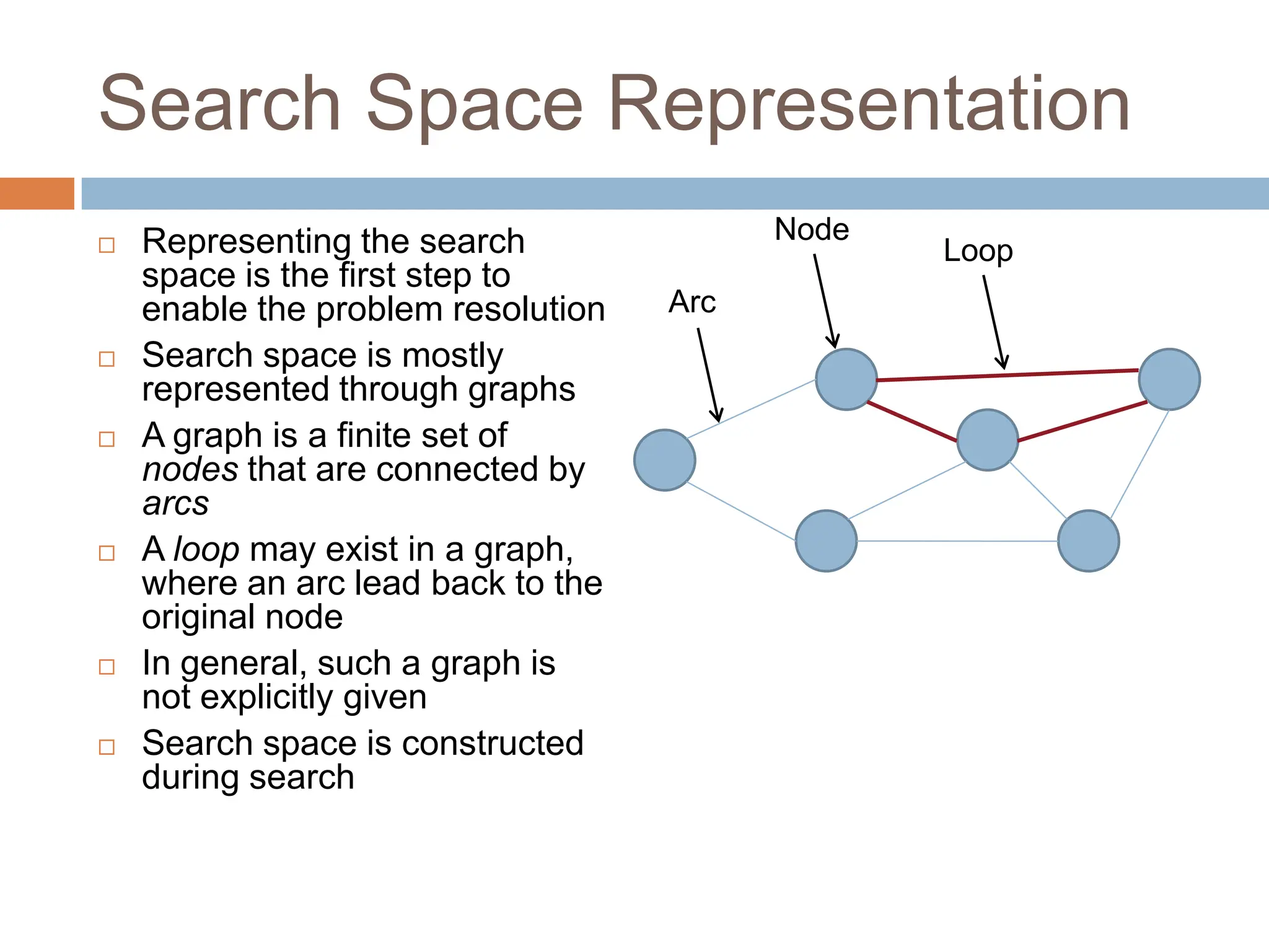
Representing the search
space is the first step to
enable the problem resolution
Search space is mostly
represented through graphs
A graph is a finite set of
nodes that are connected by
arcs
A loop may exist in a graph,
where an arc lead back to the
original node
In general, such a graph is
not explicitly given
Search space is constructed
during search
Loop
Node
Arc
8.
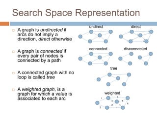
Search Space Representation
A graph is undirected if
arcs do not imply a
direction, direct otherwise
A graph is connected if
every pair of nodes is
connected by a path
A connected graph with no
loop is called tree
A weighted graph, is a
graph for which a value is
associated to each arc
undirect direct
connected disconnected
tree
weighted
1
2
4
1
5
6
2
1
1
9.
Example: Towers ofHanoi*
3
2
1
A B C
3
2
A B C
3
2
A B C
1 1
* A partial tree search space representation
3
A B C
1
2 3
2
A B C
1
…
3
A B C
1
2
A B C
1
2 3
3
A B C
1
2
…
…
3
A B C
1 2
…
3
A B C
1
2 3
A B C
1
2
…
…
…
… …
…
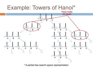
These nodes
are equals
10.
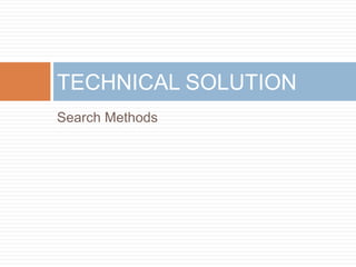
Example: Towers ofHanoi*
* A complete direct graph representation
[http://en.wikipedia.org/wiki/Tower_of_Hanoi]
11.
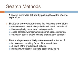
Search Methods
Asearch method is defined by picking the order of node
expansion
Strategies are evaluated along the following dimensions:
completeness: does it always find a solution if one exists?
time complexity: number of nodes generated
space complexity: maximum number of nodes in memory
optimality: does it always find the shortest path solution?
Time and space complexity are measured in terms of
b: maximum branching factor of the search tree
d: depth of the shortest path solution
m: maximum depth of the state space (may be ∞)
12.
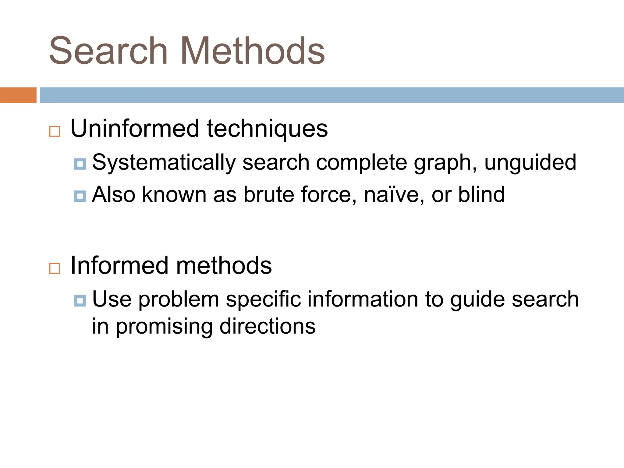
Search Methods
Uninformedtechniques
Systematically search complete graph, unguided
Also known as brute force, naïve, or blind
Informed methods
Use problem specific information to guide search
in promising directions
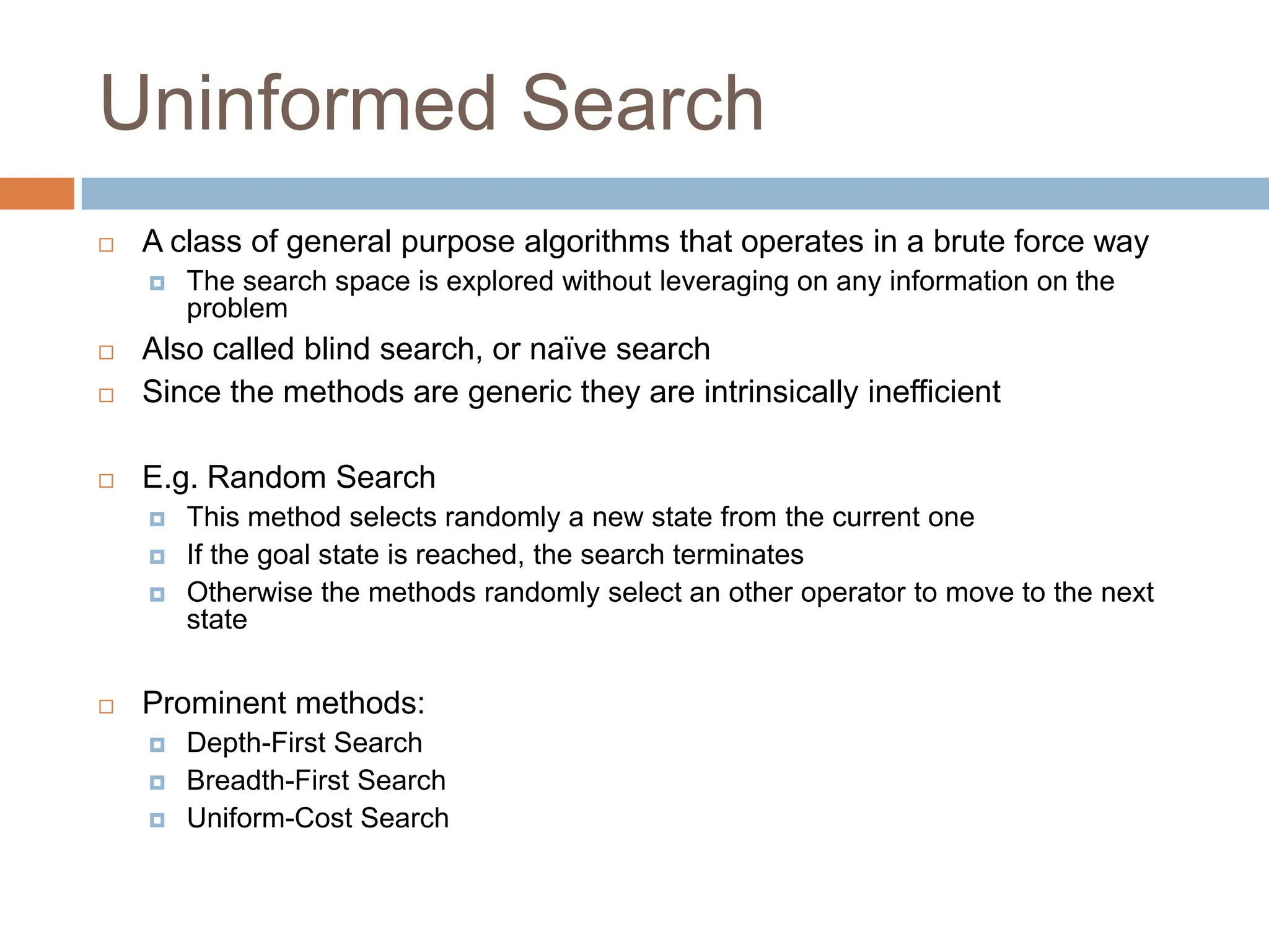
Uninformed Search
Aclass of general purpose algorithms that operates in a brute force way
The search space is explored without leveraging on any information on the
problem
Also called blind search, or naïve search
Since the methods are generic they are intrinsically inefficient
E.g. Random Search
This method selects randomly a new state from the current one
If the goal state is reached, the search terminates
Otherwise the methods randomly select an other operator to move to the next
state
Prominent methods:
Depth-First Search
Breadth-First Search
Uniform-Cost Search
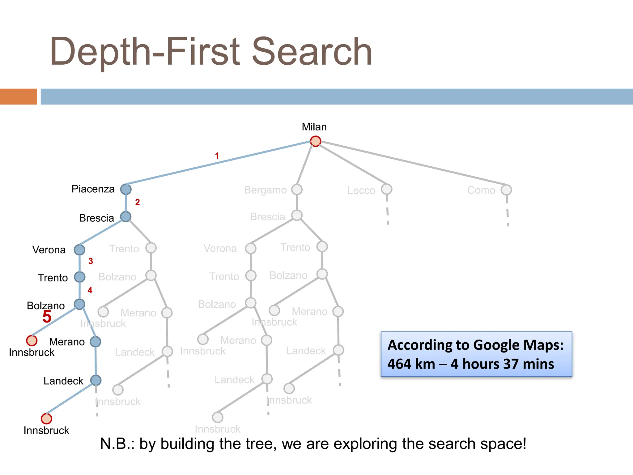
15.
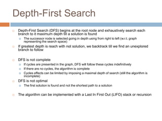
Depth-First Search
Depth-FirstSearch (DFS) begins at the root node and exhaustively search each
branch to it maximum depth till a solution is found
The successor node is selected going in depth using from right to left (w.r.t. graph
representing the search space)
If greatest depth is reach with not solution, we backtrack till we find an unexplored
branch to follow
DFS is not complete
If cycles are presented in the graph, DFS will follow these cycles indefinitively
If there are no cycles, the algorithm is complete
Cycles effects can be limited by imposing a maximal depth of search (still the algorithm is
incomplete)
DFS is not optimal
The first solution is found and not the shortest path to a solution
The algorithm can be implemented with a Last In First Out (LIFO) stack or recursion
16.
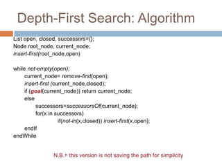
Depth-First Search: Algorithm
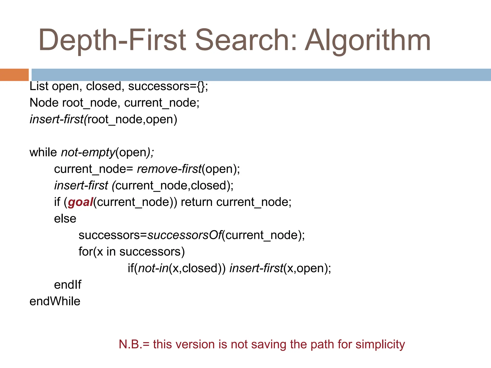
Listopen, closed, successors={};
Node root_node, current_node;
insert-first(root_node,open)
while not-empty(open);
current_node= remove-first(open);
insert-first (current_node,closed);
if (goal(current_node)) return current_node;
else
successors=successorsOf(current_node);
for(x in successors)
if(not-in(x,closed)) insert-first(x,open);
endIf
endWhile
N.B.= this version is not saving the path for simplicity
17.
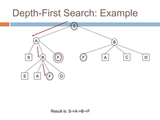
Depth-First Search: Example
S
AB
S B
S A D
F
F
1
2
3
4
5
6
A C D
F
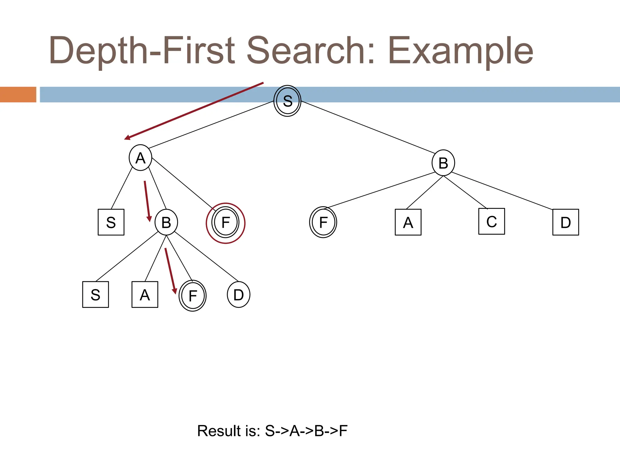
open={S} closed ={}
0. Visit S: open={A,B}, closed={S}
1.Visit A: open={S,B,F,B}, closed={A,S}
2.Visit S: open={B,F,B}, closed={S,A,S}
3.Visit B: open={S,A,F,D,F,B}, closed={B,S,A,S}
4.Visit S: open={A,F,D,F,B}, closed={S,B,S,A,S}
5.Visit A: open={F,D,F,B}, closed={A,S,B,S,A,S}
6.Visit F: GOAL Reached!
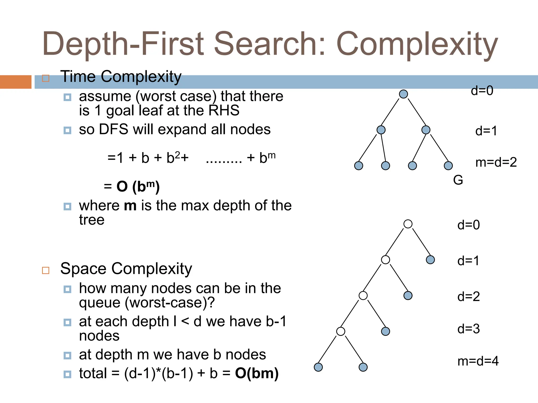
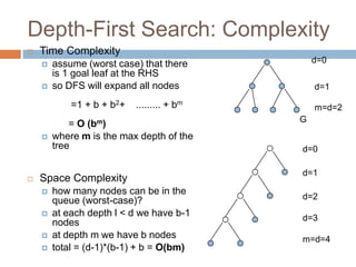
Depth-First Search: Complexity
Time Complexity
assume (worst case) that there
is 1 goal leaf at the RHS
so DFS will expand all nodes
=1 + b + b2+ ......... + bm
= O (bm)
where m is the max depth of the
tree
Space Complexity
how many nodes can be in the
queue (worst-case)?
at each depth l < d we have b-1
nodes
at depth m we have b nodes
total = (d-1)*(b-1) + b = O(bm)
d=0
d=1
m=d=2
G
d=0
d=1
d=2
d=3
m=d=4
20.
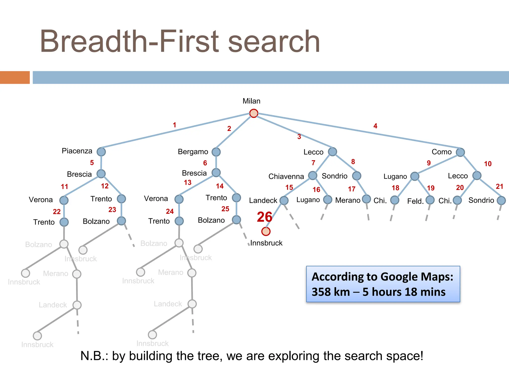
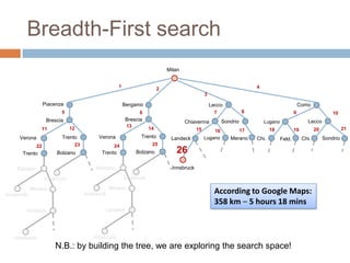
Breadth-First Search
Breadth-FirstSearch (BFS) begins at the root
node and explore level-wise al the branches
BFS is complete
If there is a solution, BFS will found it
BFS is optimal
The solution found is guaranteed to be the shortest
path possible
The algorithm can be implemented with a First In
First Out (FIFO) stack
21.
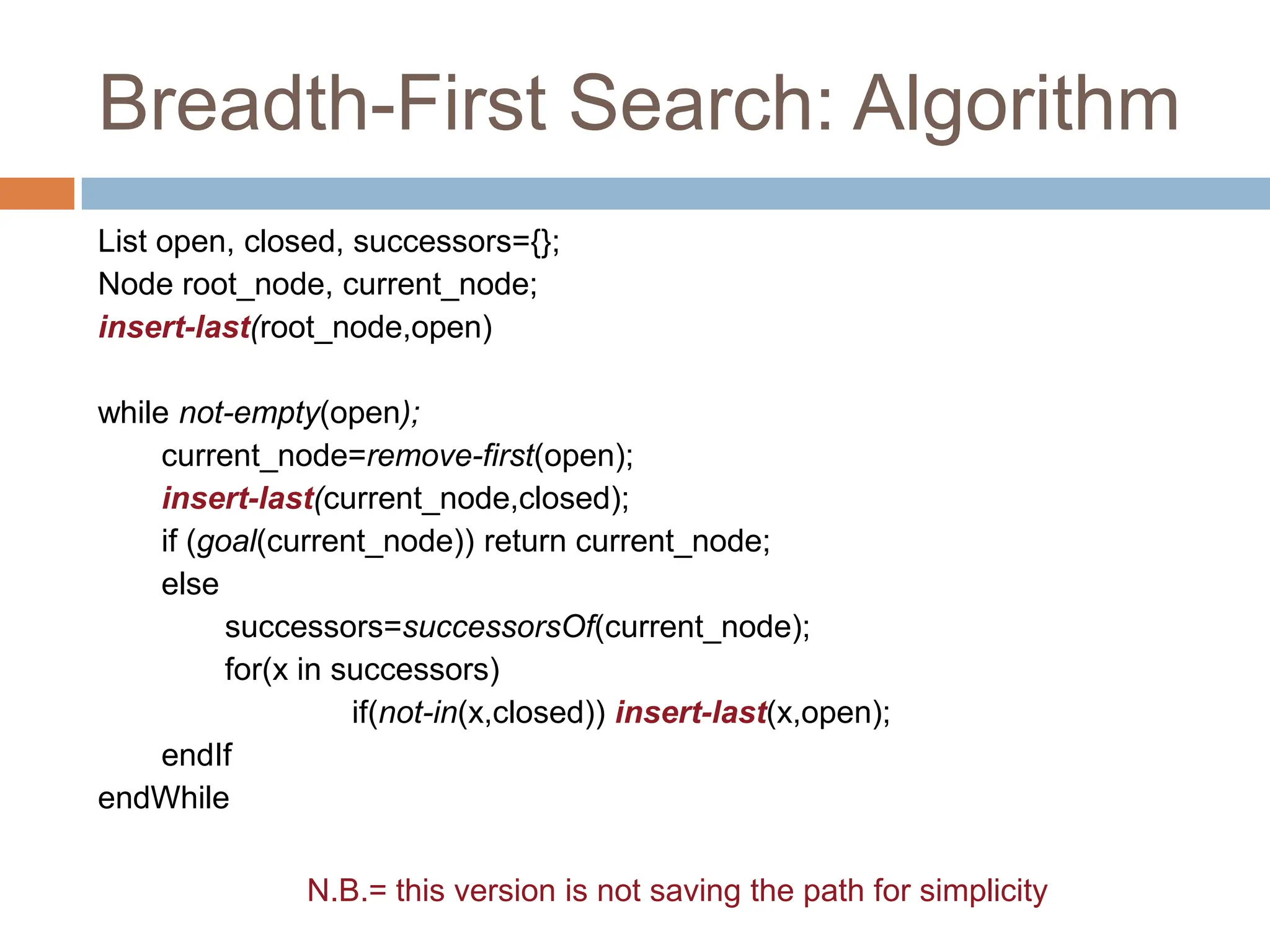
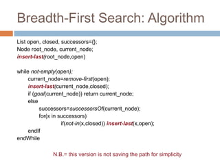
Breadth-First Search: Algorithm
Listopen, closed, successors={};
Node root_node, current_node;
insert-last(root_node,open)
while not-empty(open);
current_node=remove-first(open);
insert-last(current_node,closed);
if (goal(current_node)) return current_node;
else
successors=successorsOf(current_node);
for(x in successors)
if(not-in(x,closed)) insert-last(x,open);
endIf
endWhile
N.B.= this version is not saving the path for simplicity
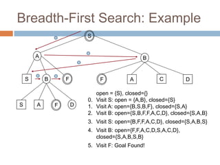
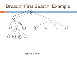
22.
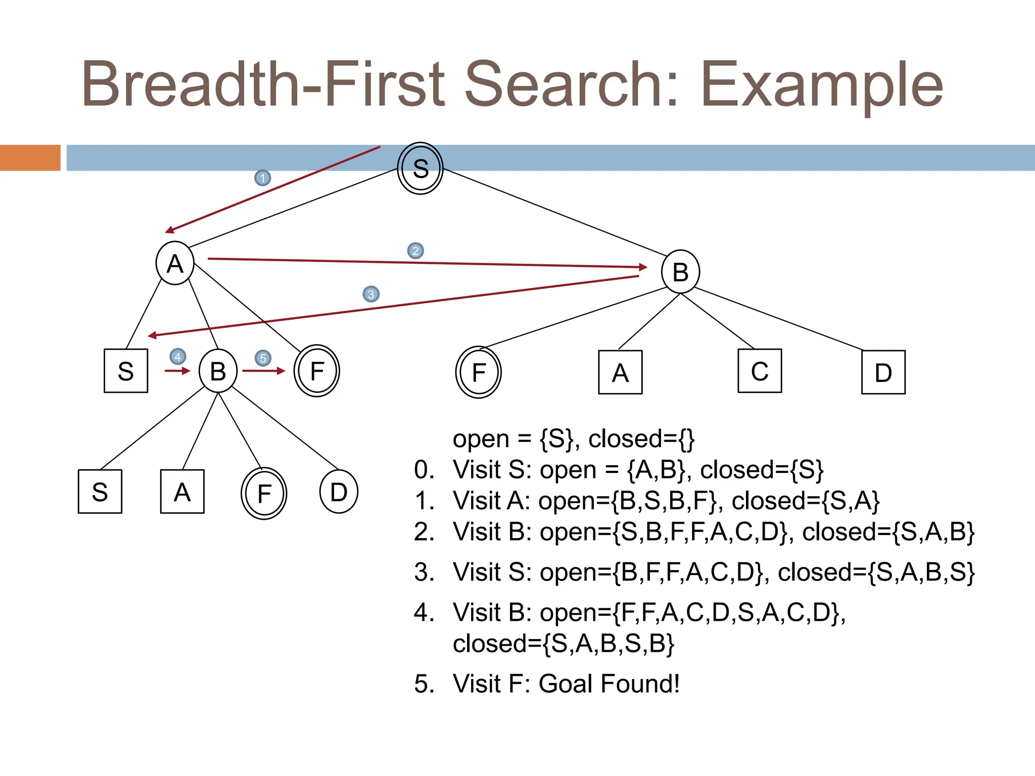
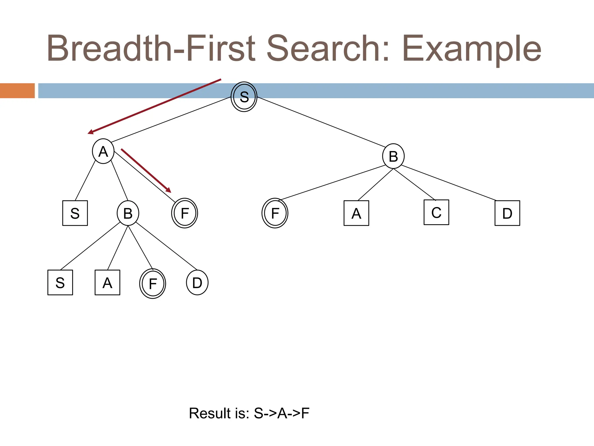
Breadth-First Search: Example
S
AB
S B
S A D
F
F
1
2
3
4 5
open = {S}, closed={}
0. Visit S: open = {A,B}, closed={S}
1. Visit A: open={B,S,B,F}, closed={S,A}
2. Visit B: open={S,B,F,F,A,C,D}, closed={S,A,B}
3. Visit S: open={B,F,F,A,C,D}, closed={S,A,B,S}
4. Visit B: open={F,F,A,C,D,S,A,C,D},
closed={S,A,B,S,B}
5. Visit F: Goal Found!
A C D
F
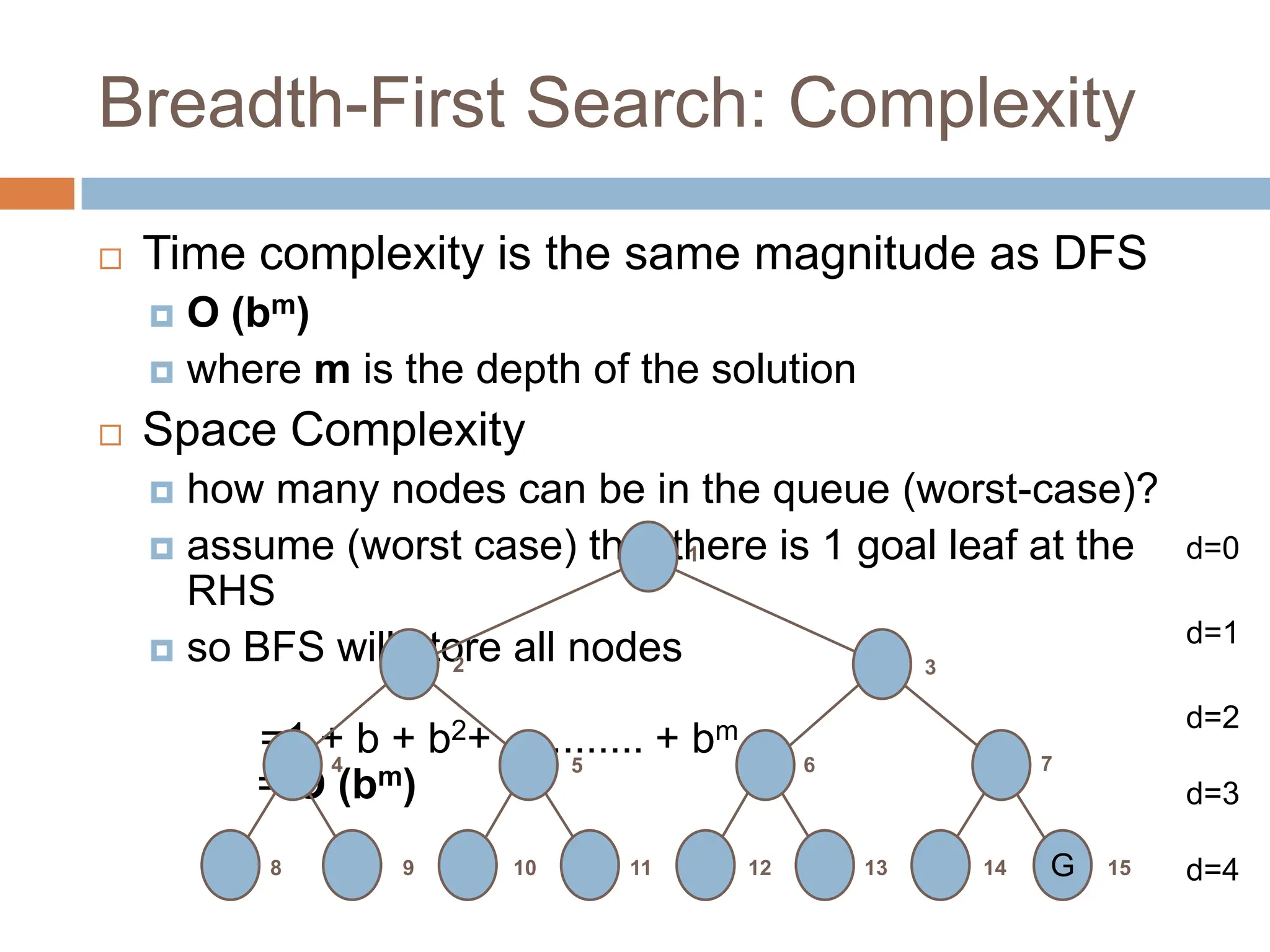
Breadth-First Search: Complexity
Time complexity is the same magnitude as DFS
O (bm)
where m is the depth of the solution
Space Complexity
how many nodes can be in the queue (worst-case)?
assume (worst case) that there is 1 goal leaf at the
RHS
so BFS will store all nodes
=1 + b + b2+ ......... + bm
= O (bm)
1
3
7
15
14
13
12
11
10
9
8
4 5 6
2
d=0
d=1
d=2
d=3
d=4
G
25.
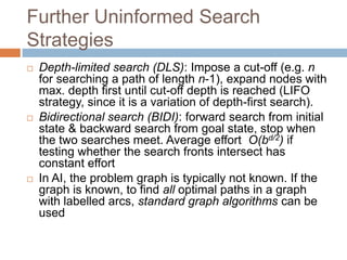
Further Uninformed Search
Strategies
Depth-limited search (DLS): Impose a cut-off (e.g. n
for searching a path of length n-1), expand nodes with
max. depth first until cut-off depth is reached (LIFO
strategy, since it is a variation of depth-first search).
Bidirectional search (BIDI): forward search from initial
state & backward search from goal state, stop when
the two searches meet. Average effort O(bd/2) if
testing whether the search fronts intersect has
constant effort
In AI, the problem graph is typically not known. If the
graph is known, to find all optimal paths in a graph
with labelled arcs, standard graph algorithms can be
used
26.
Using knowledge onthe search space to
reduce search costs
INFORMED SEARCH
27.
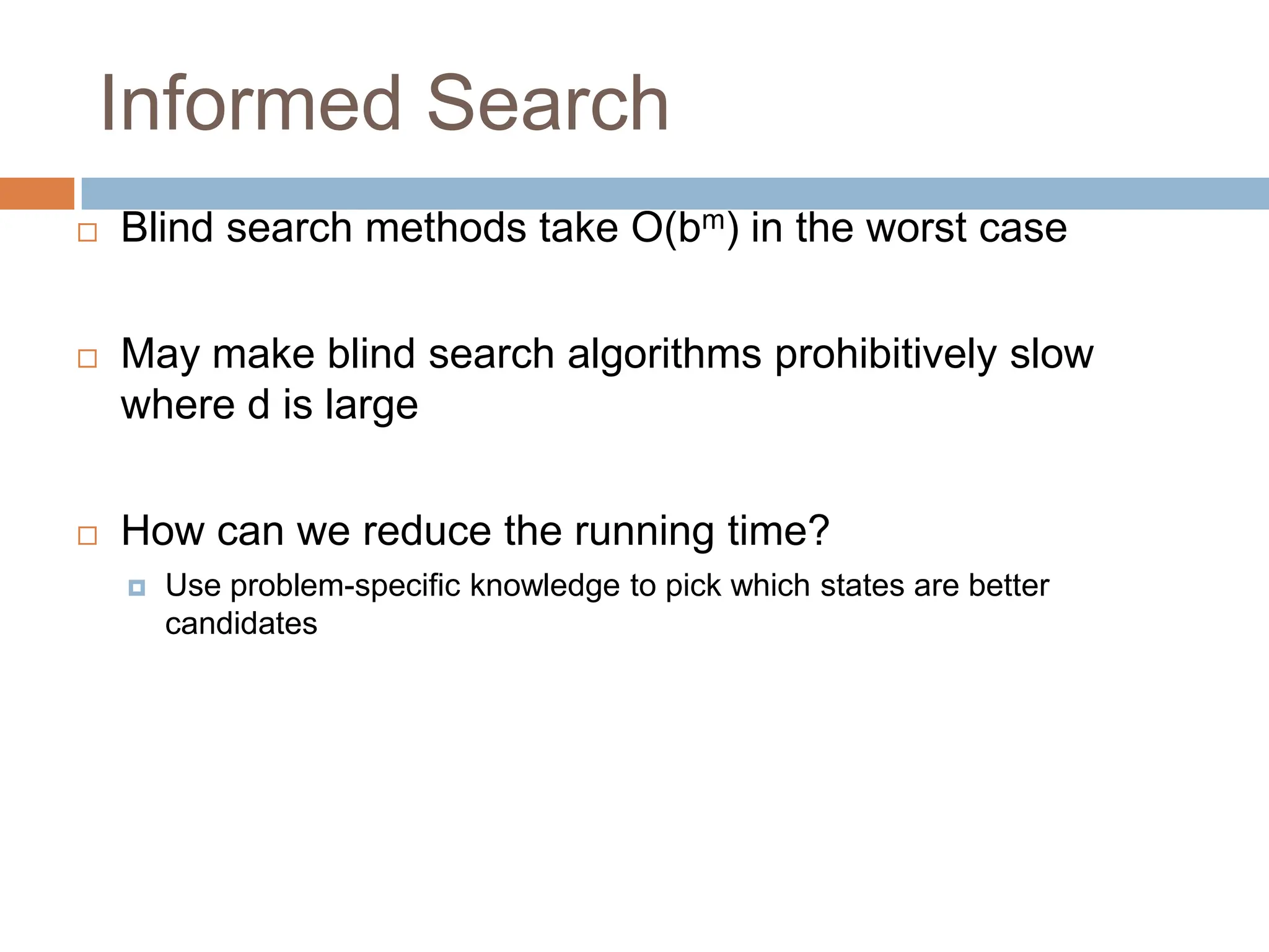
Informed Search
Blindsearch methods take O(bm) in the worst case
May make blind search algorithms prohibitively slow
where d is large
How can we reduce the running time?
Use problem-specific knowledge to pick which states are better
candidates
28.
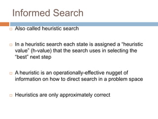
Informed Search
Alsocalled heuristic search
In a heuristic search each state is assigned a “heuristic
value” (h-value) that the search uses in selecting the
“best” next step
A heuristic is an operationally-effective nugget of
information on how to direct search in a problem space
Heuristics are only approximately correct
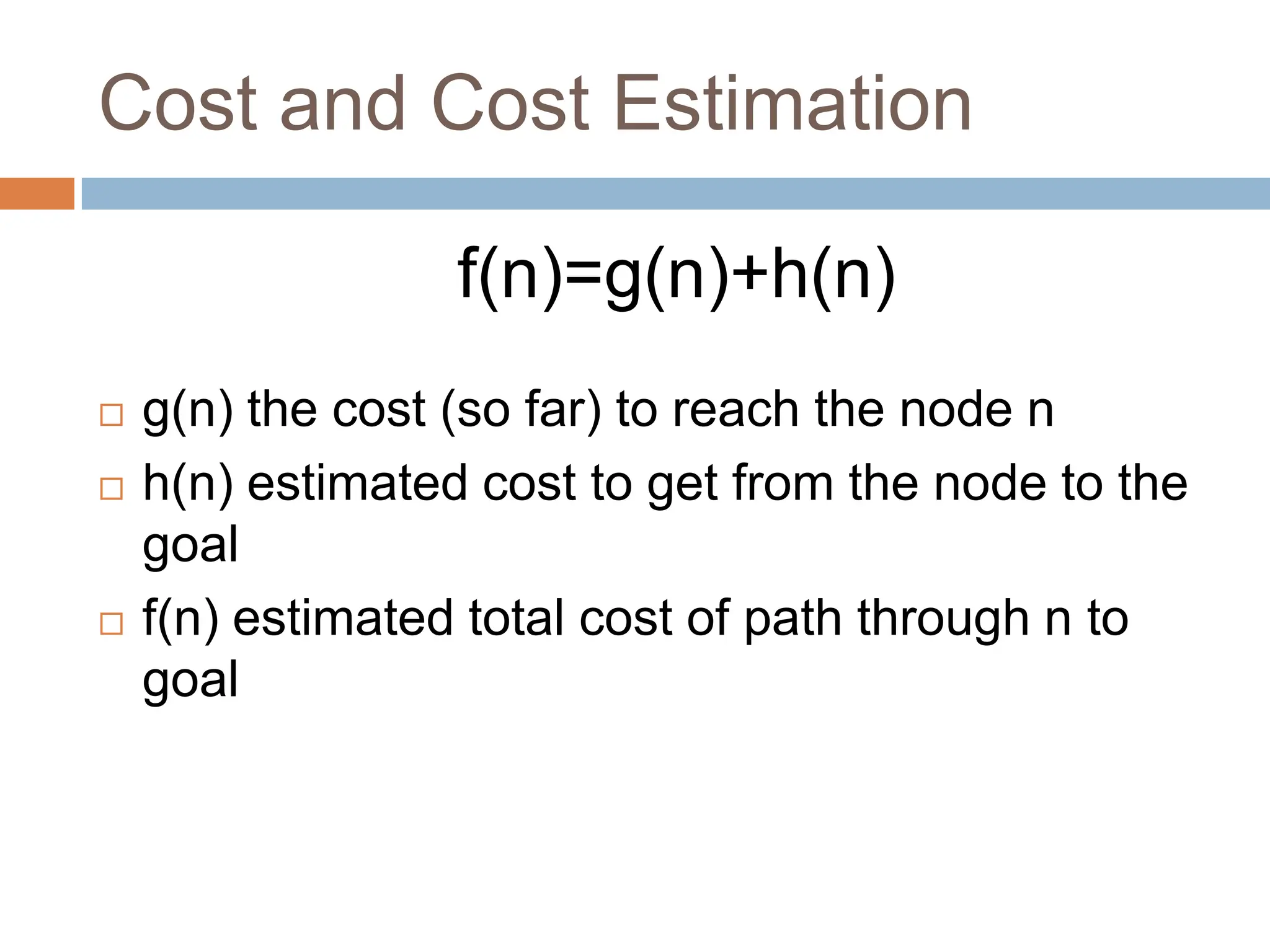
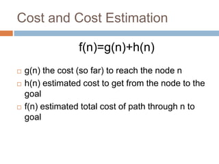
Cost and CostEstimation
f(n)=g(n)+h(n)
g(n) the cost (so far) to reach the node n
h(n) estimated cost to get from the node to the
goal
f(n) estimated total cost of path through n to
goal
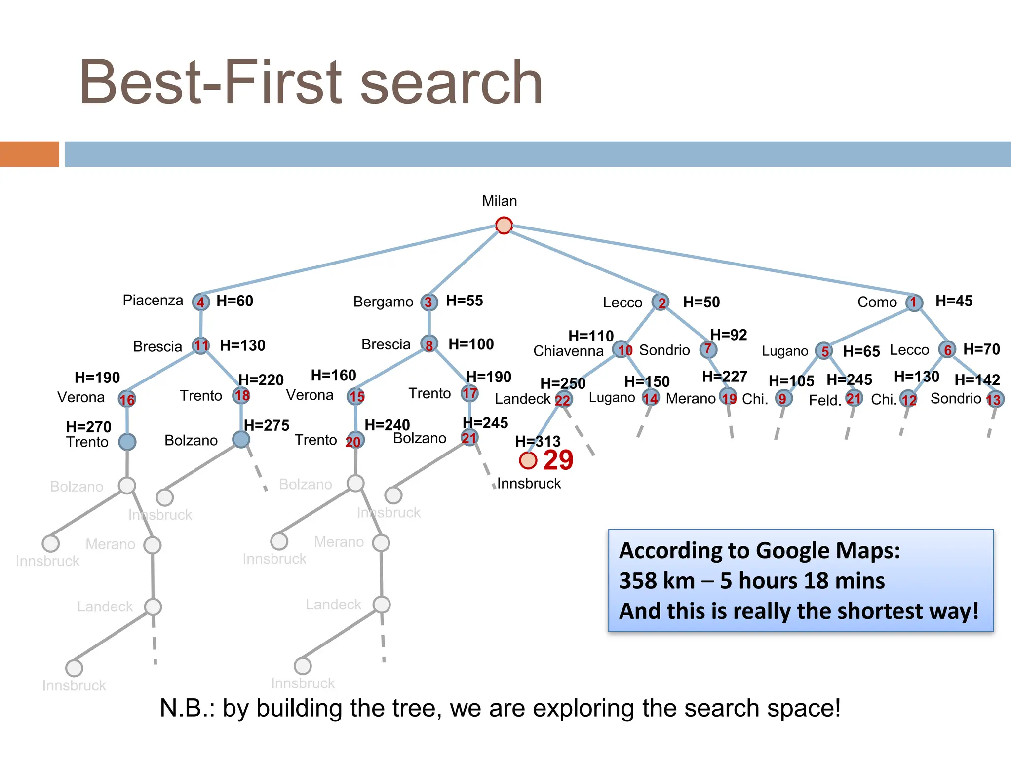
31.
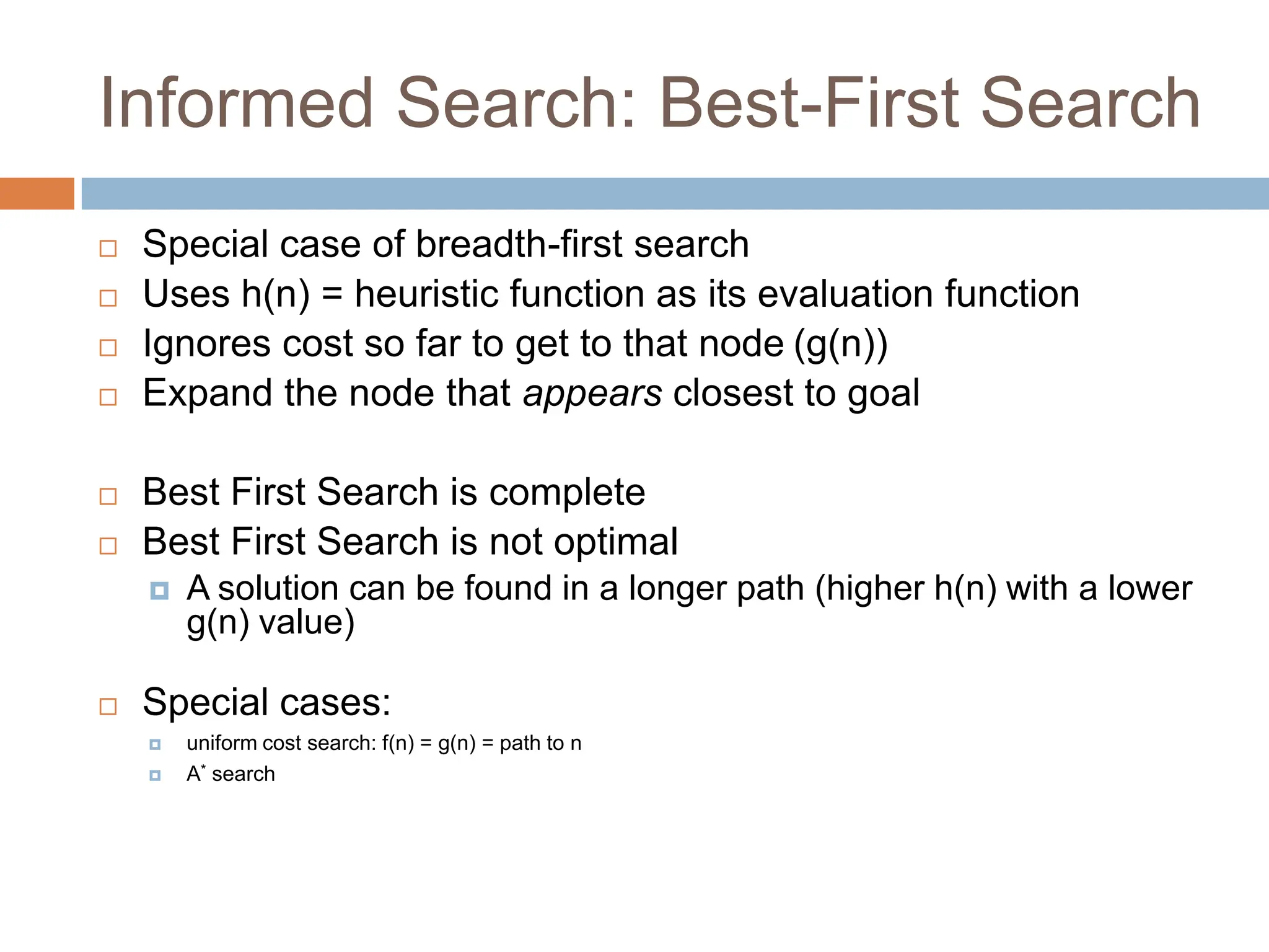
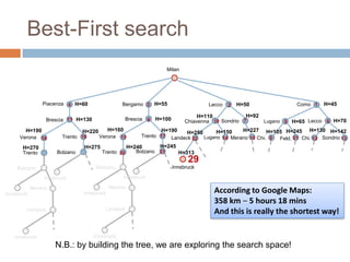
Informed Search: Best-FirstSearch
Special case of breadth-first search
Uses h(n) = heuristic function as its evaluation function
Ignores cost so far to get to that node (g(n))
Expand the node that appears closest to goal
Best First Search is complete
Best First Search is not optimal
A solution can be found in a longer path (higher h(n) with a lower
g(n) value)
Special cases:
uniform cost search: f(n) = g(n) = path to n
A* search
31
32.
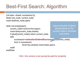
Best-First Search: Algorithm
Listopen, closed, successors={};
Node root_node, current_node;
insert-last(root_node,open)
while not-empty(open);
current_node=remove-first (open);
insert-last(current_node,closed);
if (goal(current_node)) return current_node;
else
successors=estimationOrderedSuccessorsOf(current_node);
for(x in successors)
if(not-in(x,closed)) insert-last(x,open);
endIf
endWhile
32
N.B.= this version is not saving the path for simplicity
returns the list of direct
descendants of the
current node in shortest
cost order
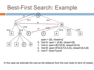
33.
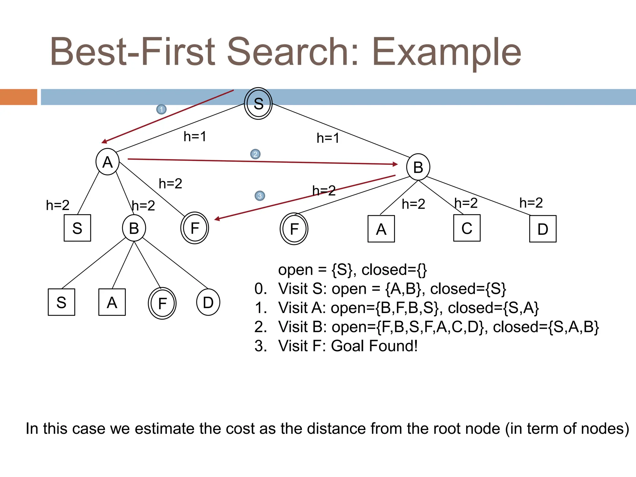
Best-First Search: Example
33
S
AB
S B
S A D
F
F
1
2
3
open = {S}, closed={}
0. Visit S: open = {A,B}, closed={S}
1. Visit A: open={B,F,B,S}, closed={S,A}
2. Visit B: open={F,B,S,F,A,C,D}, closed={S,A,B}
3. Visit F: Goal Found!
A C D
F
h=1 h=1
h=2
h=2
h=2 h=2
h=2
h=2
h=2
In this case we estimate the cost as the distance from the root node (in term of nodes)
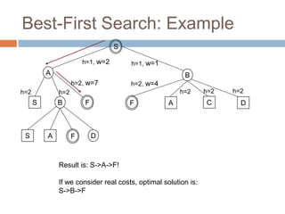
34.
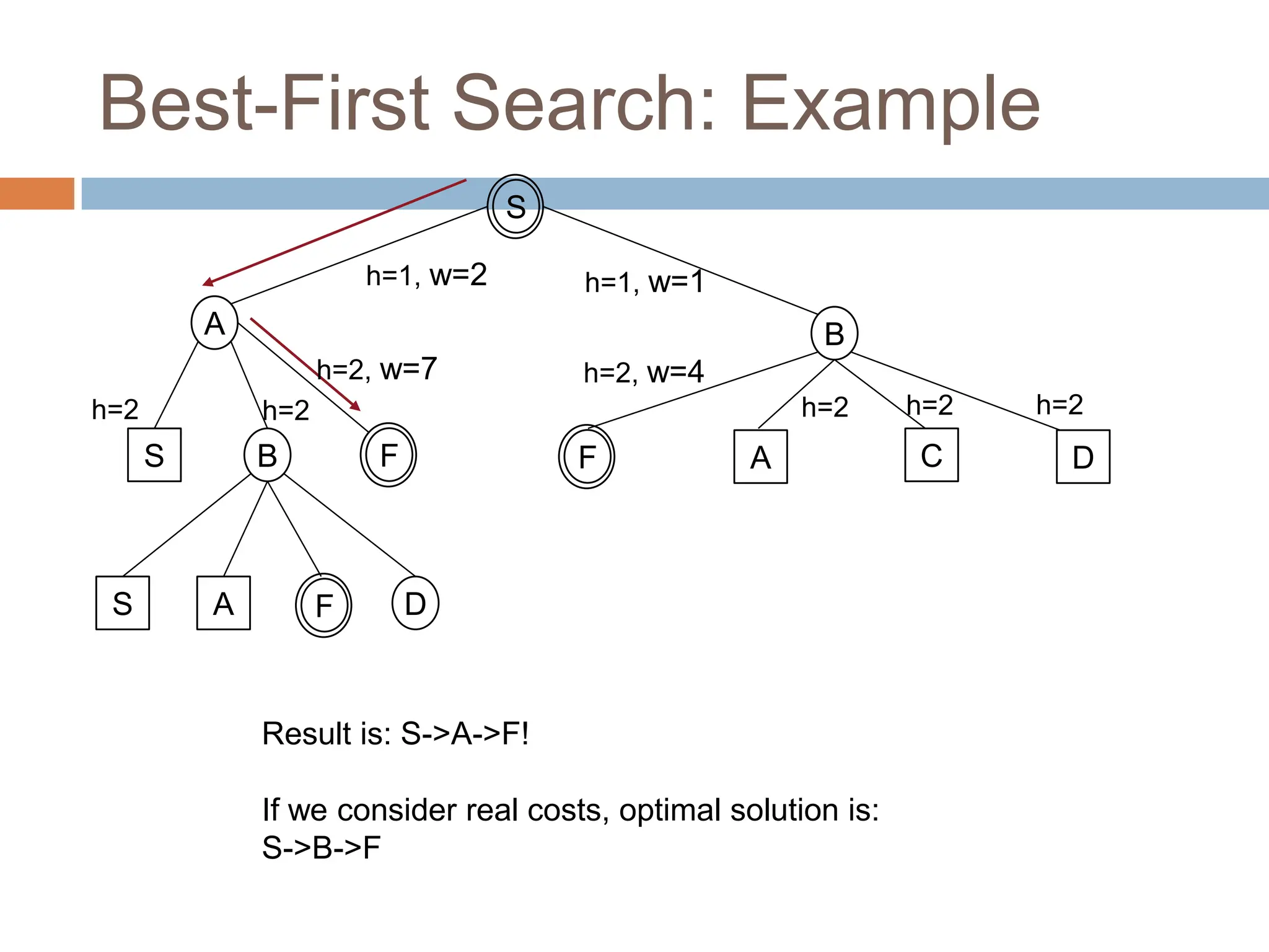
Best-First Search: Example
34
S
AB
S B
S A D
F
F A C D
F
Result is: S->A->F!
If we consider real costs, optimal solution is:
S->B->F
h=1, w=2 h=1, w=1
h=2, w=4
h=2
h=2 h=2
h=2, w=7
h=2
h=2
35.
A*
Derived fromBest-First Search
Uses both g(n) and h(n)
A* is optimal
A* is complete
36.
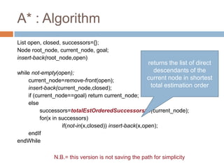
A* : Algorithm
Listopen, closed, successors={};
Node root_node, current_node, goal;
insert-back(root_node,open)
while not-empty(open);
current_node=remove-front(open);
insert-back(current_node,closed);
if (current_node==goal) return current_node;
else
successors=totalEstOrderedSuccessorsOf(current_node);
for(x in successors)
if(not-in(x,closed)) insert-back(x,open);
endIf
endWhile
36
N.B.= this version is not saving the path for simplicity
returns the list of direct
descendants of the
current node in shortest
total estimation order
37.
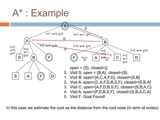
A* : Example
37
S
AB
S B
S A D
F
F
1
2
3
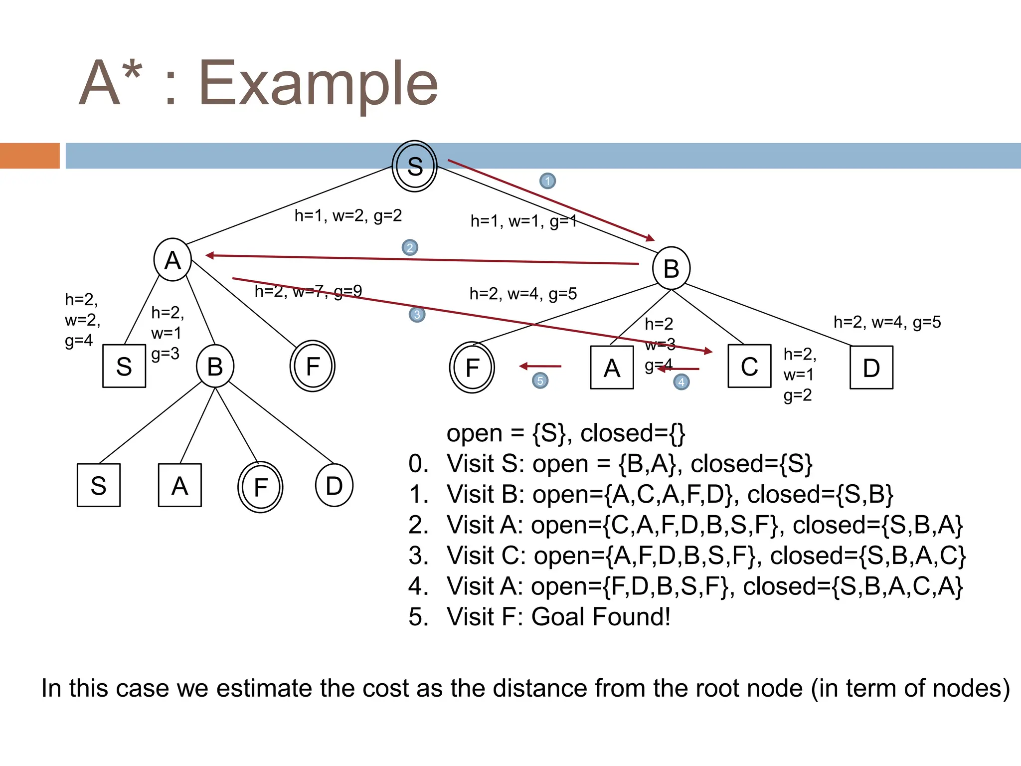
open = {S}, closed={}
0. Visit S: open = {B,A}, closed={S}
1. Visit B: open={A,C,A,F,D}, closed={S,B}
2. Visit A: open={C,A,F,D,B,S,F}, closed={S,B,A}
3. Visit C: open={A,F,D,B,S,F}, closed={S,B,A,C}
4. Visit A: open={F,D,B,S,F}, closed={S,B,A,C,A}
5. Visit F: Goal Found!
A C D
F
h=2,
w=1
g=3
h=2,
w=2,
g=4
In this case we estimate the cost as the distance from the root node (in term of nodes)
h=1, w=2, g=2 h=1, w=1, g=1
h=2, w=4, g=5
h=2, w=7, g=9
h=2,
w=1
g=2
h=2
w=3
g=4
h=2, w=4, g=5
4
5
38.
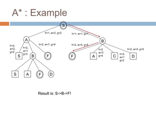
A* : Example
38
S
AB
S B
S A D
F
F A C D
F
h=2,
w=1
g=3
h=2,
w=2,
g=4
h=1, w=2, g=2 h=1, w=1, g=1
h=2, w=4, g=5
h=2, w=7, g=9
h=2,
w=1
g=2
h=2
w=3
g=4
h=2, w=4, g=5
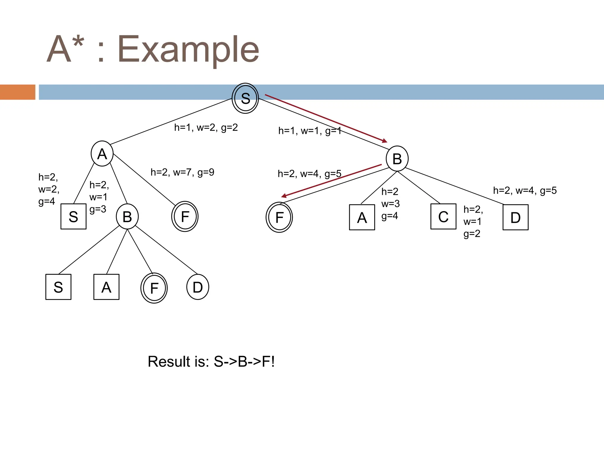
Result is: S->B->F!
39.
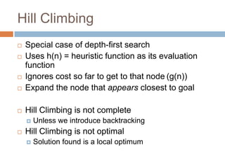
Hill Climbing
Specialcase of depth-first search
Uses h(n) = heuristic function as its evaluation
function
Ignores cost so far to get to that node (g(n))
Expand the node that appears closest to goal
Hill Climbing is not complete
Unless we introduce backtracking
Hill Climbing is not optimal
Solution found is a local optimum
40.
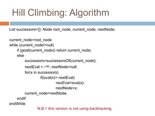
Hill Climbing: Algorithm
Listsuccessors={}; Node root_node, current_node, nextNode;
current_node=root_node
while (current_node!=null)
if (goal(current_node)) return current_node;
else
successors=successorsOf(current_node);
nextEval = -∞; nextNode=null;
for(x in successors)
if(eval(x)> nextEval)
nexEval=eval(x);
nextNode=x;
current_node=nextNode,
endIf
endWhile
40
N.B.= this version is not using backtracking
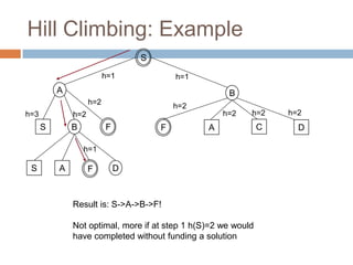
41.
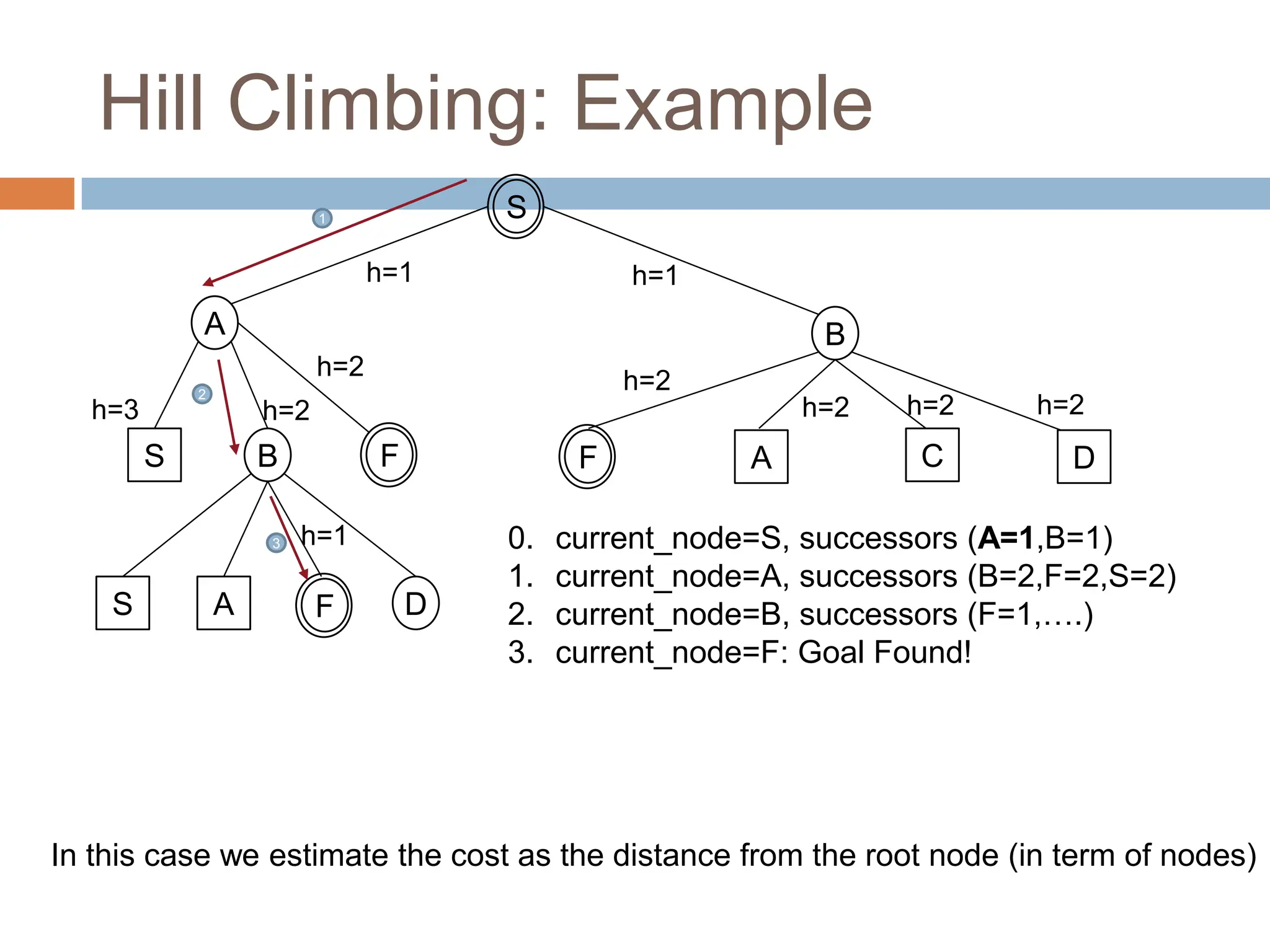
Hill Climbing: Example
41
S
AB
S B
S A D
F
F
1
2
3 0. current_node=S, successors (A=1,B=1)
1. current_node=A, successors (B=2,F=2,S=2)
2. current_node=B, successors (F=1,….)
3. current_node=F: Goal Found!
A C D
F
h=1 h=1
h=2
h=2
h=2 h=2
h=2
h=2
h=3
In this case we estimate the cost as the distance from the root node (in term of nodes)
h=1
42.
Hill Climbing: Example
42
S
AB
S B
S A D
F
F A C D
F
h=1 h=1
h=2
h=2
h=2 h=2
h=2
h=2
h=3
h=1
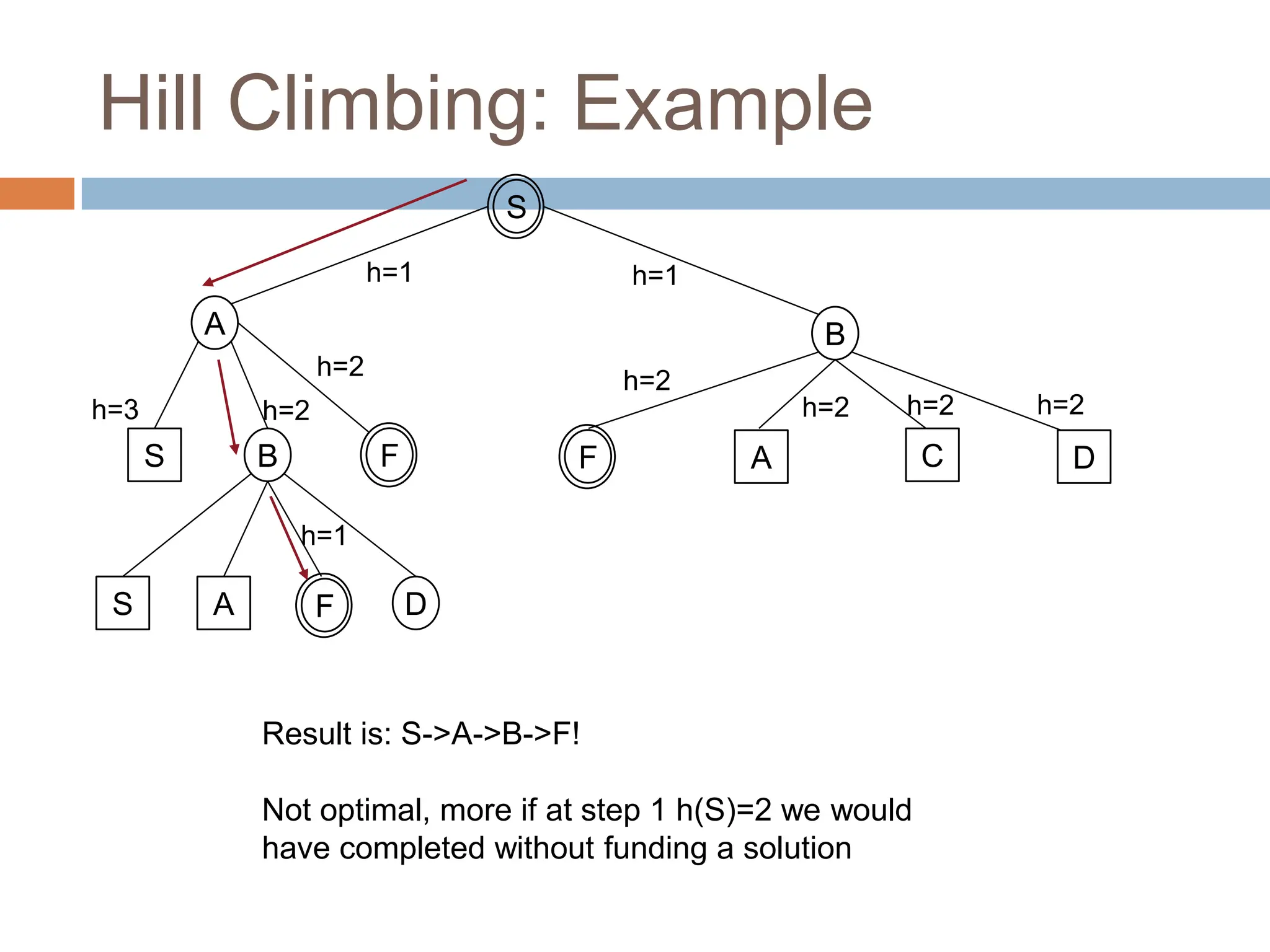
Result is: S->A->B->F!
Not optimal, more if at step 1 h(S)=2 we would
have completed without funding a solution
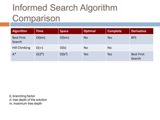
43.
Informed Search Algorithm
Comparison
AlgorithmTime Space Optimal Complete Derivative
Best First
Search
O(bm) O(bm) No Yes BFS
Hill Climbing O() O(b) No No
A* O(2N) O(bd) Yes Yes Best First
Search
43
b, branching factor
d, tree depth of the solution
m, maximum tree depth
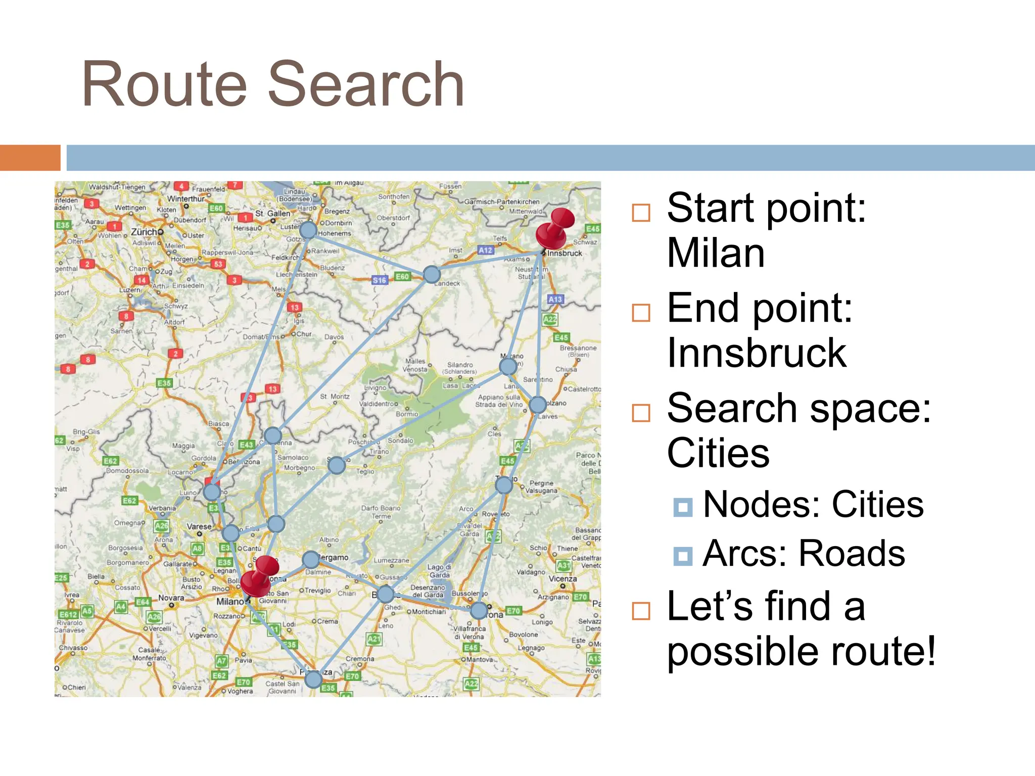
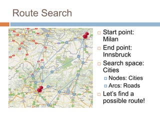
Route Search
Startpoint:
Milan
End point:
Innsbruck
Search space:
Cities
Nodes: Cities
Arcs: Roads
Let’s find a
possible route!
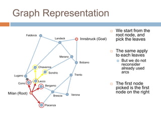
46.
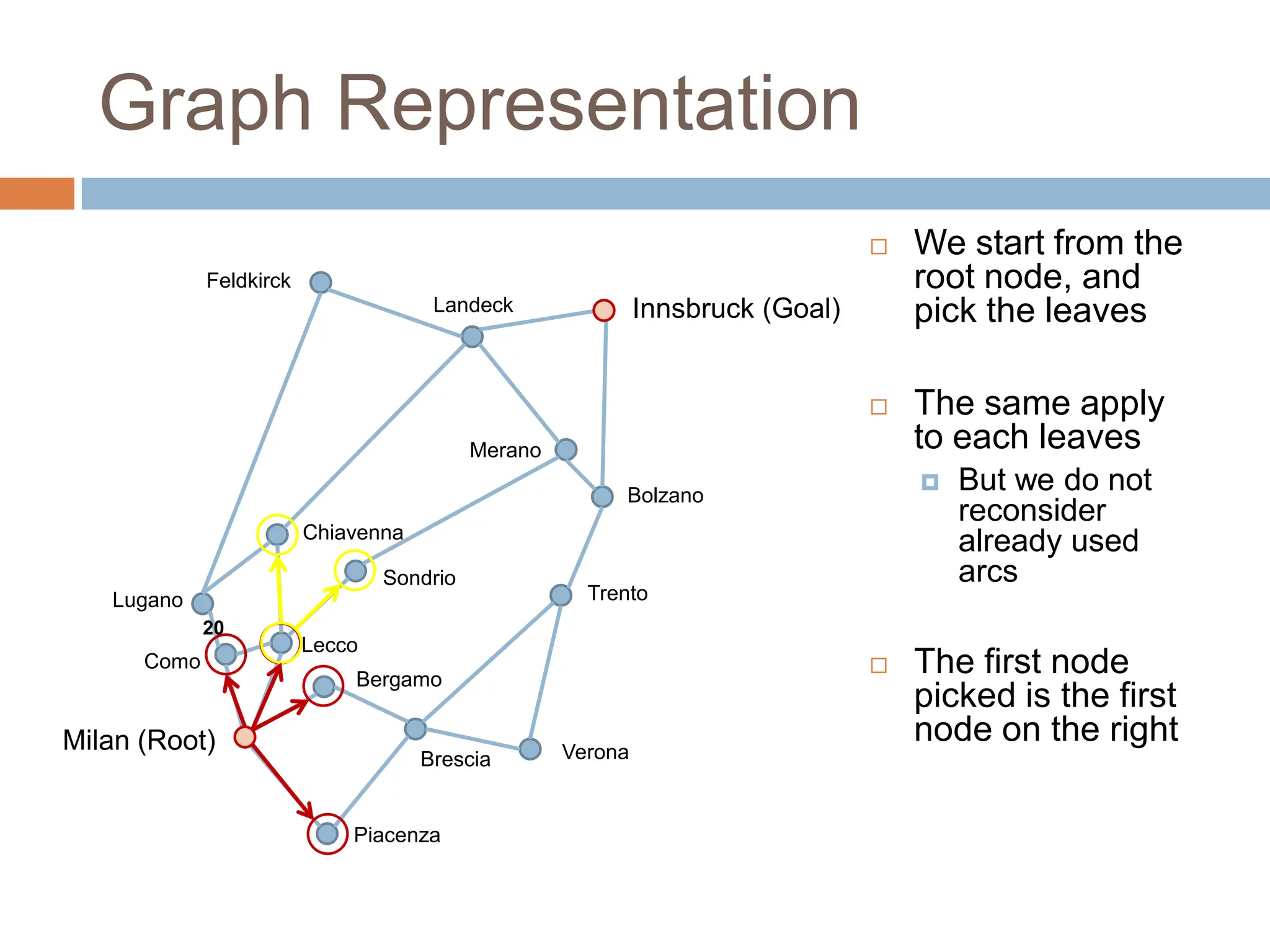
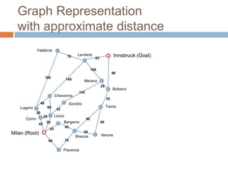
Graph Representation
Westart from the
root node, and
pick the leaves
The same apply
to each leaves
But we do not
reconsider
already used
arcs
The first node
picked is the first
node on the right
Innsbruck (Goal)
Milan (Root)
Piacenza
Verona
Bolzano
Trento
Merano
Landeck
Sondrio
Bergamo
Brescia
Lecco
Como
Lugano
Chiavenna
Feldkirck
20
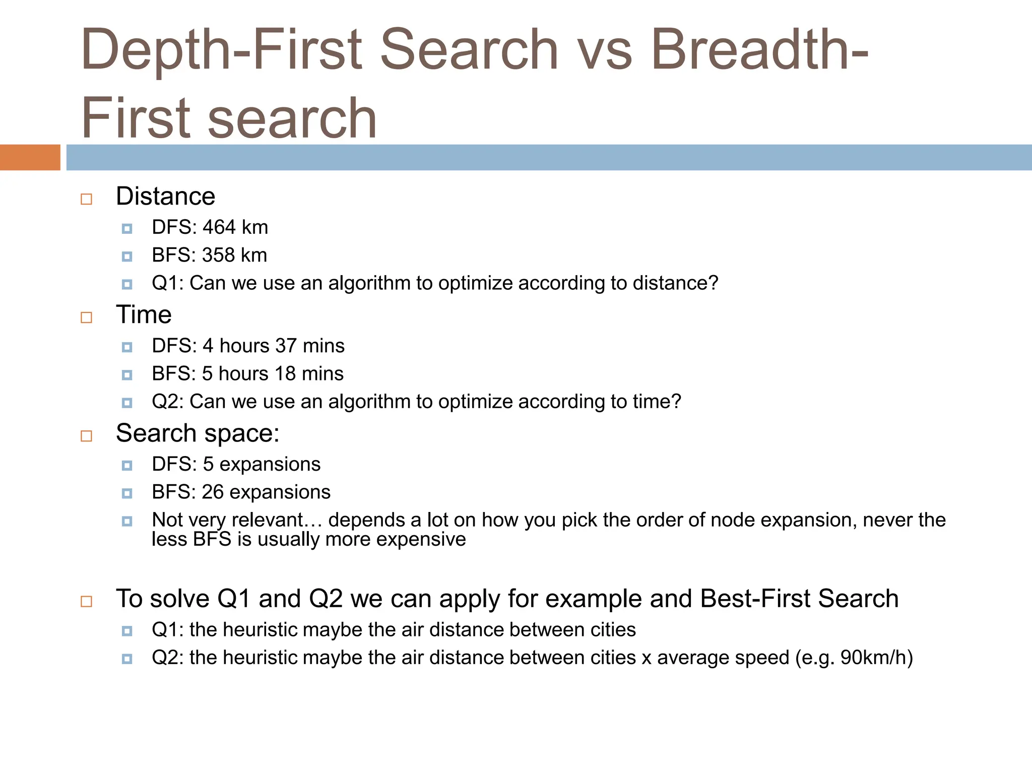
Depth-First Search vsBreadth-
First search
Distance
DFS: 464 km
BFS: 358 km
Q1: Can we use an algorithm to optimize according to distance?
Time
DFS: 4 hours 37 mins
BFS: 5 hours 18 mins
Q2: Can we use an algorithm to optimize according to time?
Search space:
DFS: 5 expansions
BFS: 26 expansions
Not very relevant… depends a lot on how you pick the order of node expansion, never the
less BFS is usually more expensive
To solve Q1 and Q2 we can apply for example and Best-First Search
Q1: the heuristic maybe the air distance between cities
Q2: the heuristic maybe the air distance between cities x average speed (e.g. 90km/h)
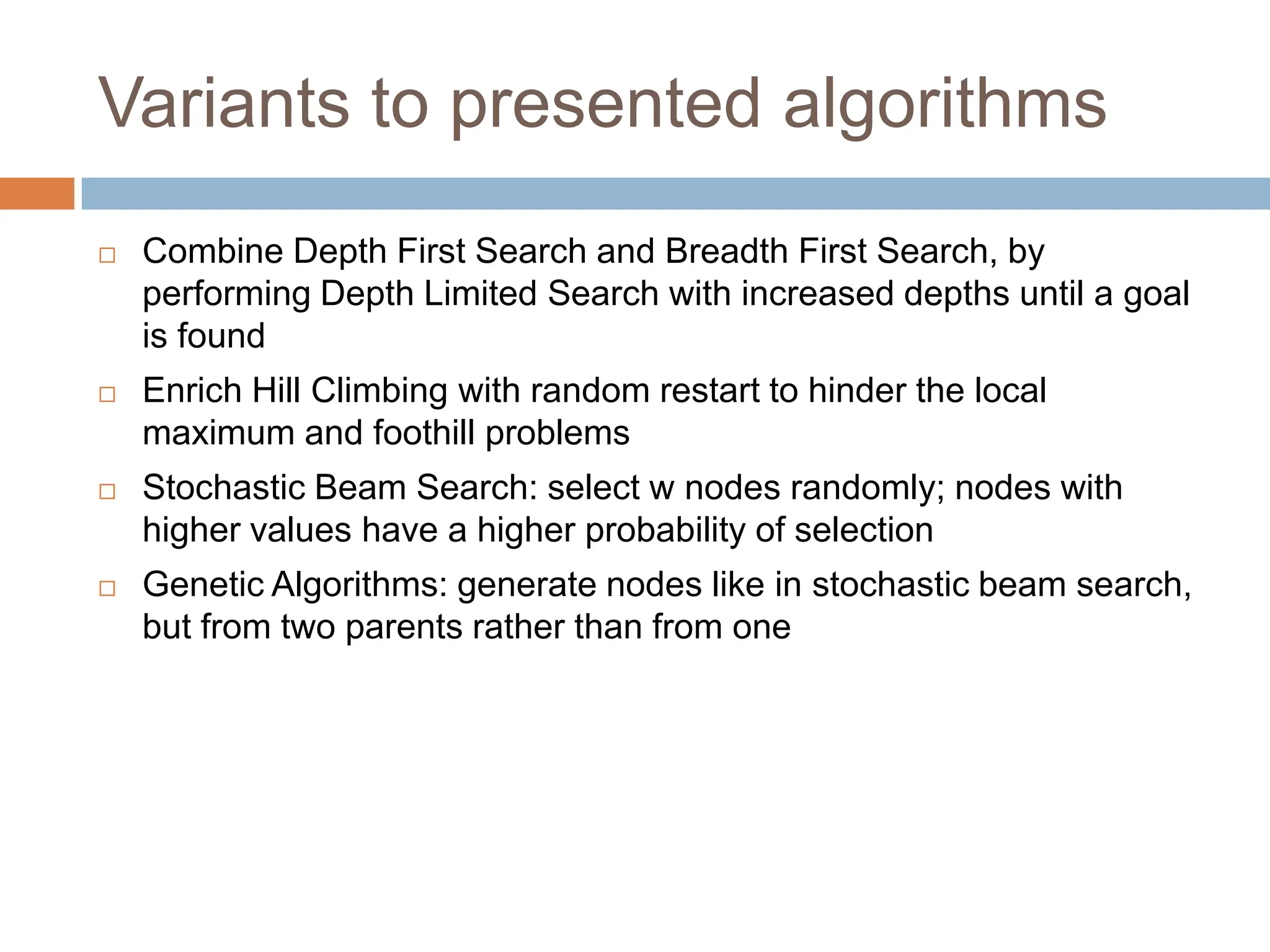
Variants to presentedalgorithms
Combine Depth First Search and Breadth First Search, by
performing Depth Limited Search with increased depths until a goal
is found
Enrich Hill Climbing with random restart to hinder the local
maximum and foothill problems
Stochastic Beam Search: select w nodes randomly; nodes with
higher values have a higher probability of selection
Genetic Algorithms: generate nodes like in stochastic beam search,
but from two parents rather than from one
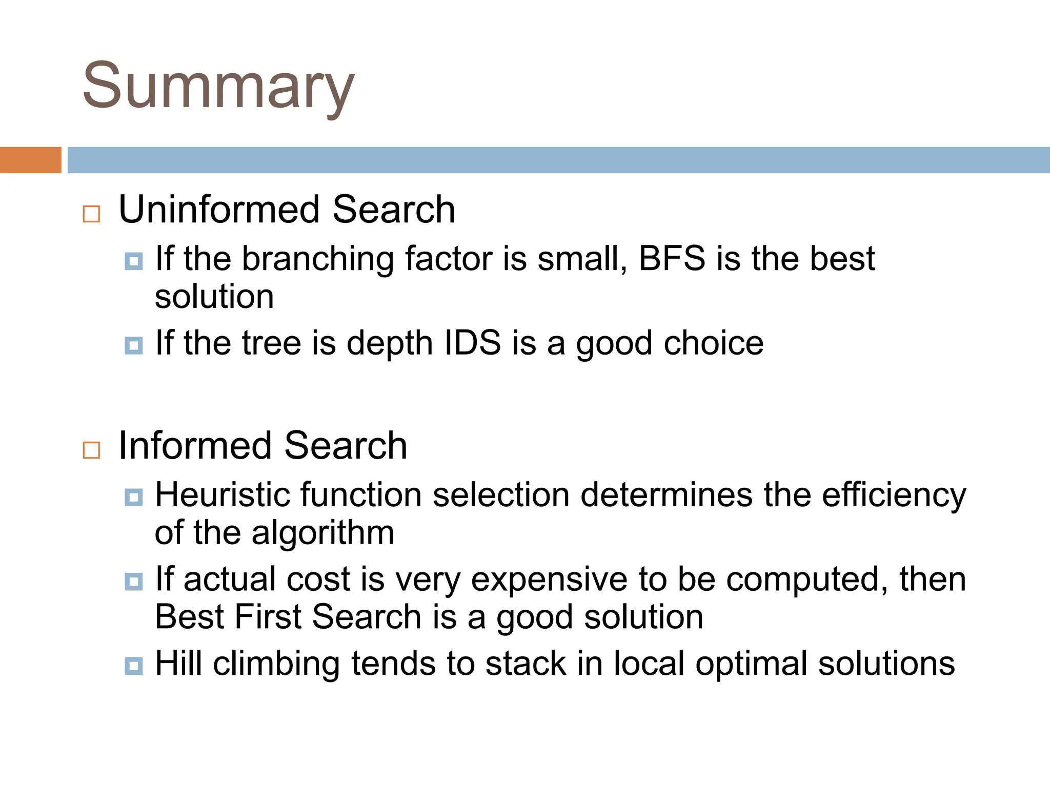
Summary
Uninformed Search
If the branching factor is small, BFS is the best
solution
If the tree is depth IDS is a good choice
Informed Search
Heuristic function selection determines the efficiency
of the algorithm
If actual cost is very expensive to be computed, then
Best First Search is a good solution
Hill climbing tends to stack in local optimal solutions


![Example: Towers of Hanoi*
* A complete direct graph representation
[http://en.wikipedia.org/wiki/Tower_of_Hanoi]](https://image.slidesharecdn.com/uninformed-and-informed-search-250908041058-78d02e12/85/UNINFORMED-AND-INFORMED-SEARCH-ALGORITHMS-10-320.jpg)


![Example: Towers of Hanoi*
* A complete direct graph representation
[http://en.wikipedia.org/wiki/Tower_of_Hanoi]](https://image.slidesharecdn.com/uninformed-and-informed-search-250908041058-78d02e12/75/UNINFORMED-AND-INFORMED-SEARCH-ALGORITHMS-10-2048.jpg)