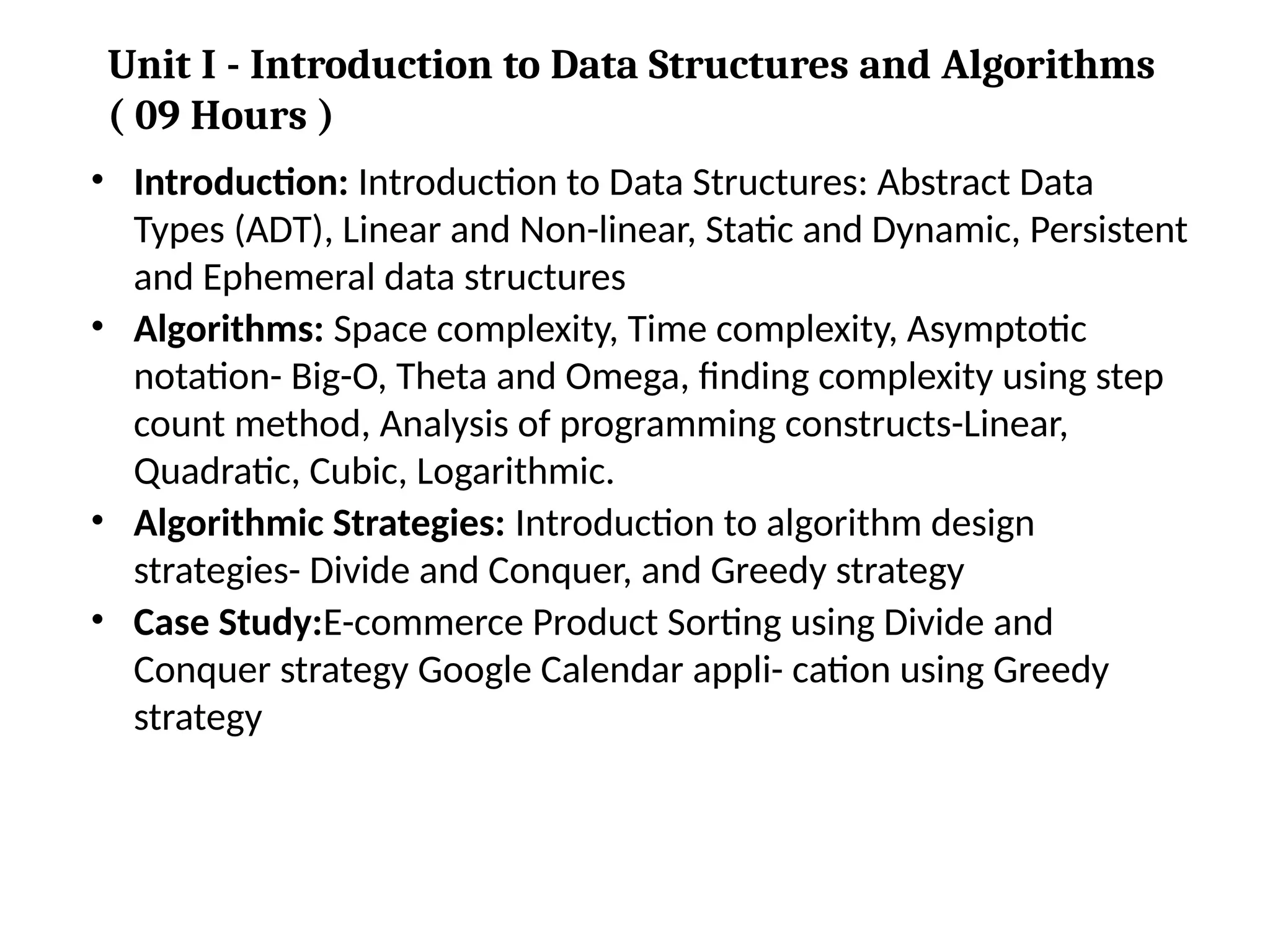
• Introduction: Introductionto Data Structures: Abstract Data
Types (ADT), Linear and Non-linear, Static and Dynamic, Persistent
and Ephemeral data structures
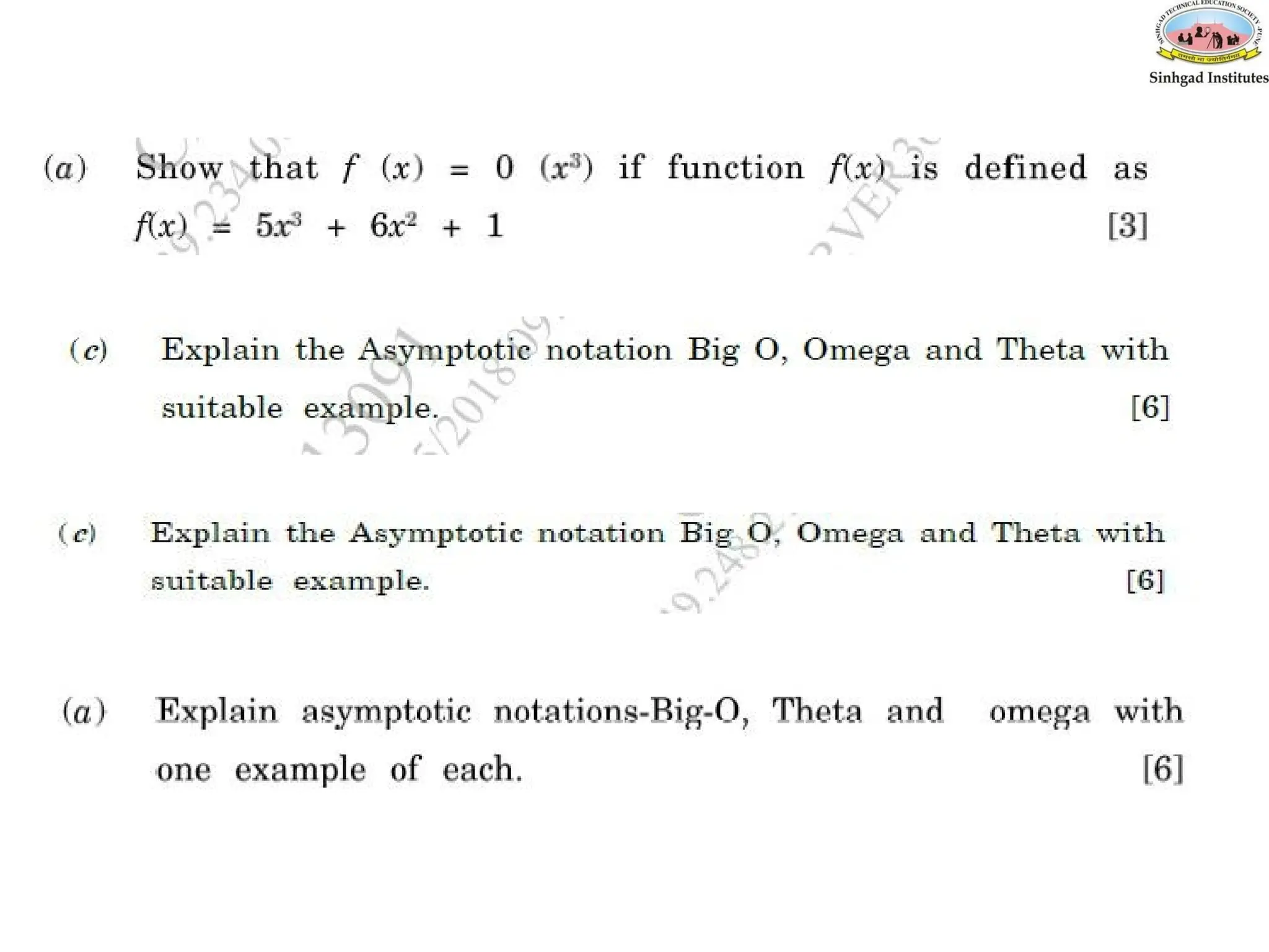
• Algorithms: Space complexity, Time complexity, Asymptotic
notation- Big-O, Theta and Omega, finding complexity using step
count method, Analysis of programming constructs-Linear,
Quadratic, Cubic, Logarithmic.
• Algorithmic Strategies: Introduction to algorithm design
strategies- Divide and Conquer, and Greedy strategy
• Case Study:E-commerce Product Sorting using Divide and
Conquer strategy Google Calendar appli- cation using Greedy
strategy
Unit I - Introduction to Data Structures and Algorithms
( 09 Hours )
3.
Algorithm
• An Algorithmis a finite sequence of instructions,
each of which has a clear meaning and can be
performed with a finite amount of effort in a
finite length of time.
• No matter what the input values may be, an
algorithm terminates after executing a finite
number of instructions.
4.
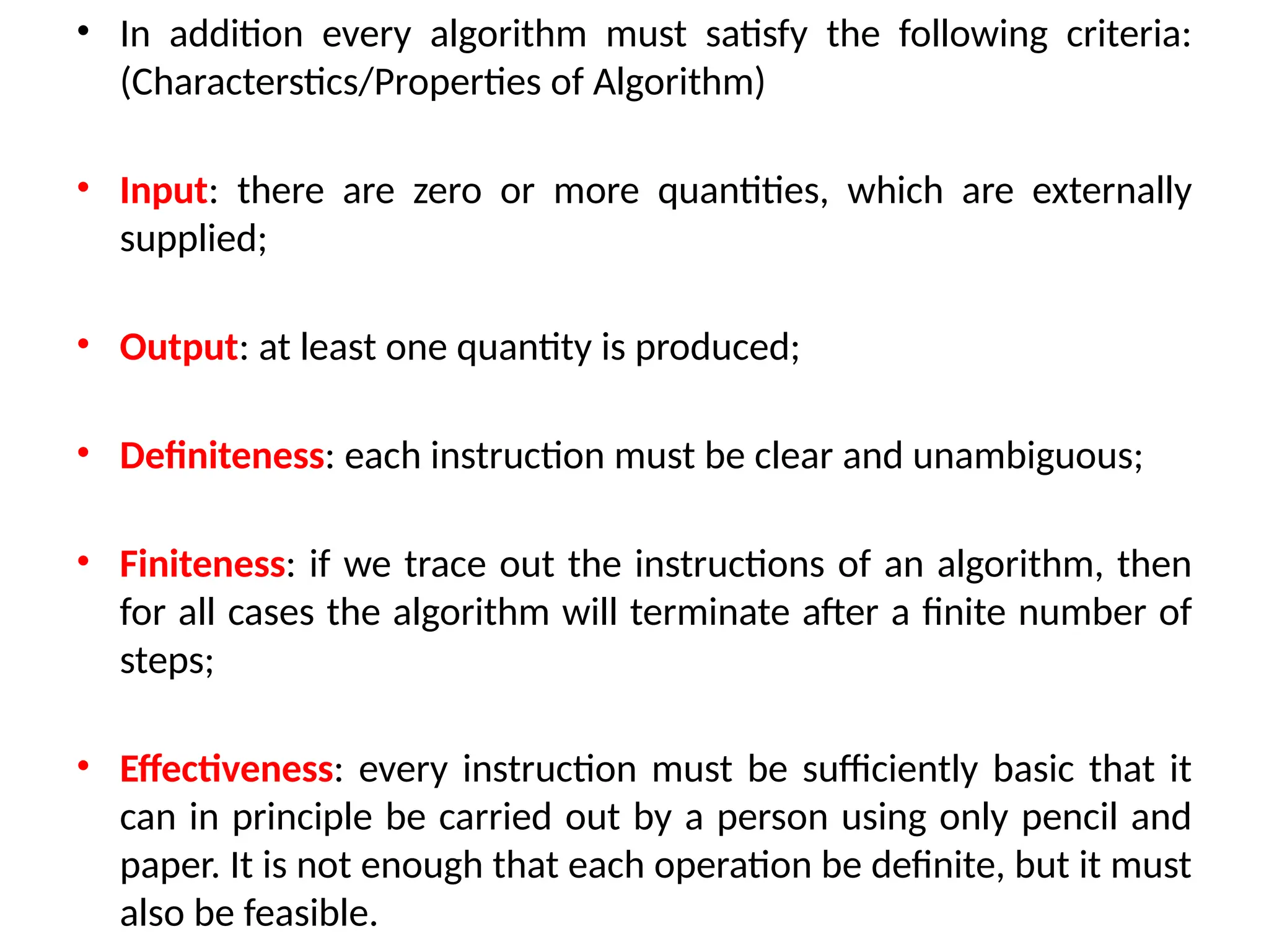
• In additionevery algorithm must satisfy the following criteria:
(Characterstics/Properties of Algorithm)
• Input: there are zero or more quantities, which are externally
supplied;
• Output: at least one quantity is produced;
• Definiteness: each instruction must be clear and unambiguous;
• Finiteness: if we trace out the instructions of an algorithm, then
for all cases the algorithm will terminate after a finite number of
steps;
• Effectiveness: every instruction must be sufficiently basic that it
can in principle be carried out by a person using only pencil and
paper. It is not enough that each operation be definite, but it must
also be feasible.
5.
• Data isa collection of numbers, alphabets and symbols
combined to represent information.
• A computer takes raw data as input and after processing of
data it produces refined data as output. We might say that
computer science is the study of data.
Atomic data:
Atomic data are non-decomposable entity. For example, an integer
value 523 or a character value 'A' cannot be further divided. If we
further divide the value 523 in three digits '5', '2' and '3' then the
meaning may be lost.
Data:
6.
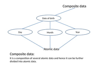
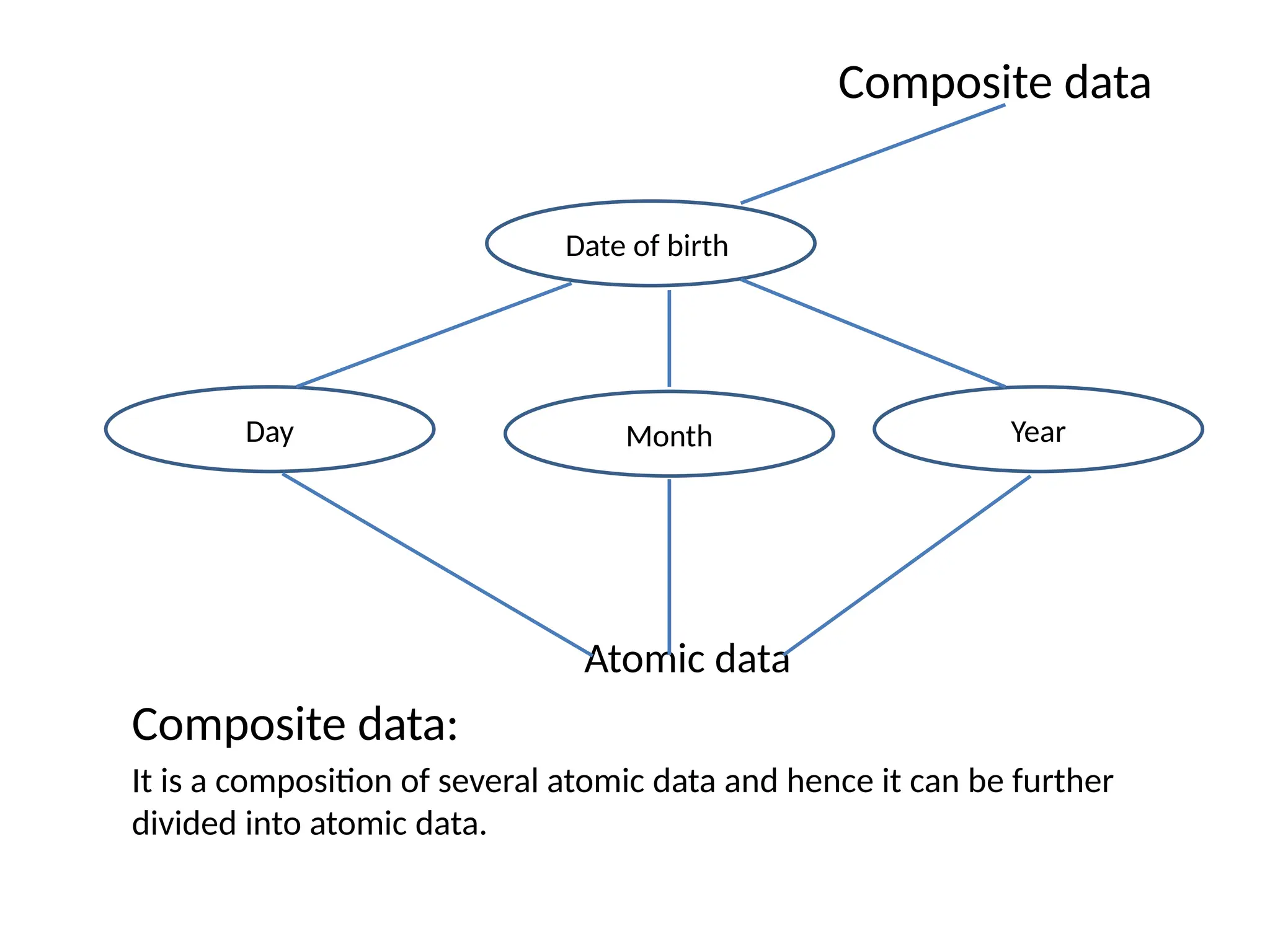
Composite data
Atomic data
Compositedata:
It is a composition of several atomic data and hence it can be further
divided into atomic data.
Date of birth
Day Month Year
7.
Information:
What is Information?
Informationis organized or classified data, which has
some meaningful values for the receiver. Information is the
processed data on which decisions and actions are based.
For the decision to be meaningful, the processed data must
qualify for the following characteristics −
•Timely − Information should be available when required.
•Accuracy − Information should be accurate.
•Completeness − Information should be complete.
8.
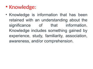
• Knowledge:
• Knowledgeis information that has been
retained with an understanding about the
significance of that information.
Knowledge includes something gained by
experience, study, familiarity, association,
awareness, and/or comprehension.
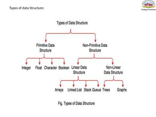
Data Types:
A datatype is a term which refers to the kind of data that
variables may hold in a programming language.
Example: int x; [x can hold, integer type data]
11.
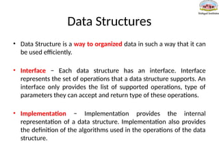
Data Structures
• DataStructure is a way to organized data in such a way that it can
be used efficiently.
• Interface − Each data structure has an interface. Interface
represents the set of operations that a data structure supports. An
interface only provides the list of supported operations, type of
parameters they can accept and return type of these operations.
• Implementation − Implementation provides the internal
representation of a data structure. Implementation also provides
the definition of the algorithms used in the operations of the data
structure.
12.
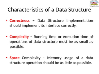
Characteristics of aData Structure
• Correctness − Data Structure implementation
should implement its interface correctly.
• Complexity − Running time or execution time of
operations of data structure must be as small as
possible.
• Space Complexity − Memory usage of a data
structure operation should be as little as possible.
13.
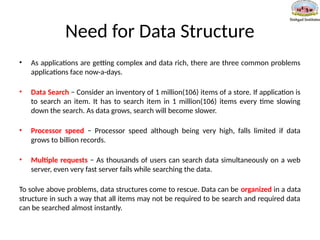
Need for DataStructure
• As applications are getting complex and data rich, there are three common problems
applications face now-a-days.
• Data Search − Consider an inventory of 1 million(106) items of a store. If application is
to search an item. It has to search item in 1 million(106) items every time slowing
down the search. As data grows, search will become slower.
• Processor speed − Processor speed although being very high, falls limited if data
grows to billion records.
• Multiple requests − As thousands of users can search data simultaneously on a web
server, even very fast server fails while searching the data.
To solve above problems, data structures come to rescue. Data can be organized in a data
structure in such a way that all items may not be required to be search and required data
can be searched almost instantly.
14.
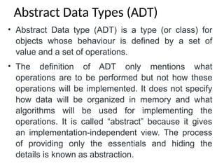
• Abstract Datatype (ADT) is a type (or class) for
objects whose behaviour is defined by a set of
value and a set of operations.
• The definition of ADT only mentions what
operations are to be performed but not how these
operations will be implemented. It does not specify
how data will be organized in memory and what
algorithms will be used for implementing the
operations. It is called “abstract” because it gives
an implementation-independent view. The process
of providing only the essentials and hiding the
details is known as abstraction.
Abstract Data Types (ADT)
15.
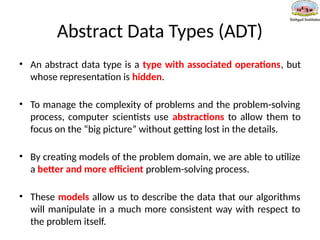
Abstract Data Types(ADT)
• An abstract data type is a type with associated operations, but
whose representation is hidden.
• To manage the complexity of problems and the problem-solving
process, computer scientists use abstractions to allow them to
focus on the “big picture” without getting lost in the details.
• By creating models of the problem domain, we are able to utilize
a better and more efficient problem-solving process.
• These models allow us to describe the data that our algorithms
will manipulate in a much more consistent way with respect to
the problem itself.
16.
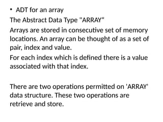
• ADT foran array
The Abstract Data Type "ARRAY“
Arrays are stored in consecutive set of memory
locations. An array can be thought of as a set of
pair, index and value.
For each index which is defined there is a value
associated with that index.
There are two operations permitted on 'ARRAY'
data structure. These two operations are
retrieve and store.
17.
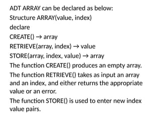
ADT ARRAY canbe declared as below:
Structure ARRAY(value, index)
declare
CREATE() → array
RETRIEVE(array, index) → value
STORE(array, index, value) → array
The function CREATE() produces an empty array.
The function RETRIEVE() takes as input an array
and an index, and either returns the appropriate
value or an error.
The function STORE() is used to enter new index
value pairs.
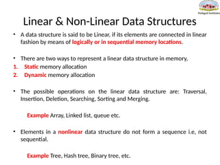
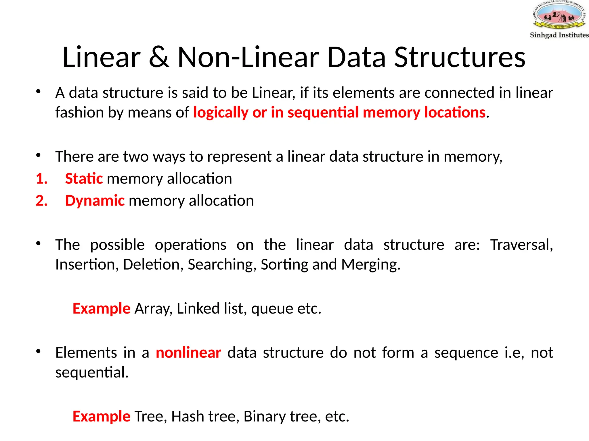
Linear & Non-LinearData Structures
• A data structure is said to be Linear, if its elements are connected in linear
fashion by means of logically or in sequential memory locations.
• There are two ways to represent a linear data structure in memory,
1. Static memory allocation
2. Dynamic memory allocation
• The possible operations on the linear data structure are: Traversal,
Insertion, Deletion, Searching, Sorting and Merging.
Example Array, Linked list, queue etc.
• Elements in a nonlinear data structure do not form a sequence i.e, not
sequential.
Example Tree, Hash tree, Binary tree, etc.
20.
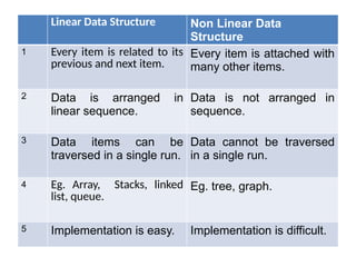
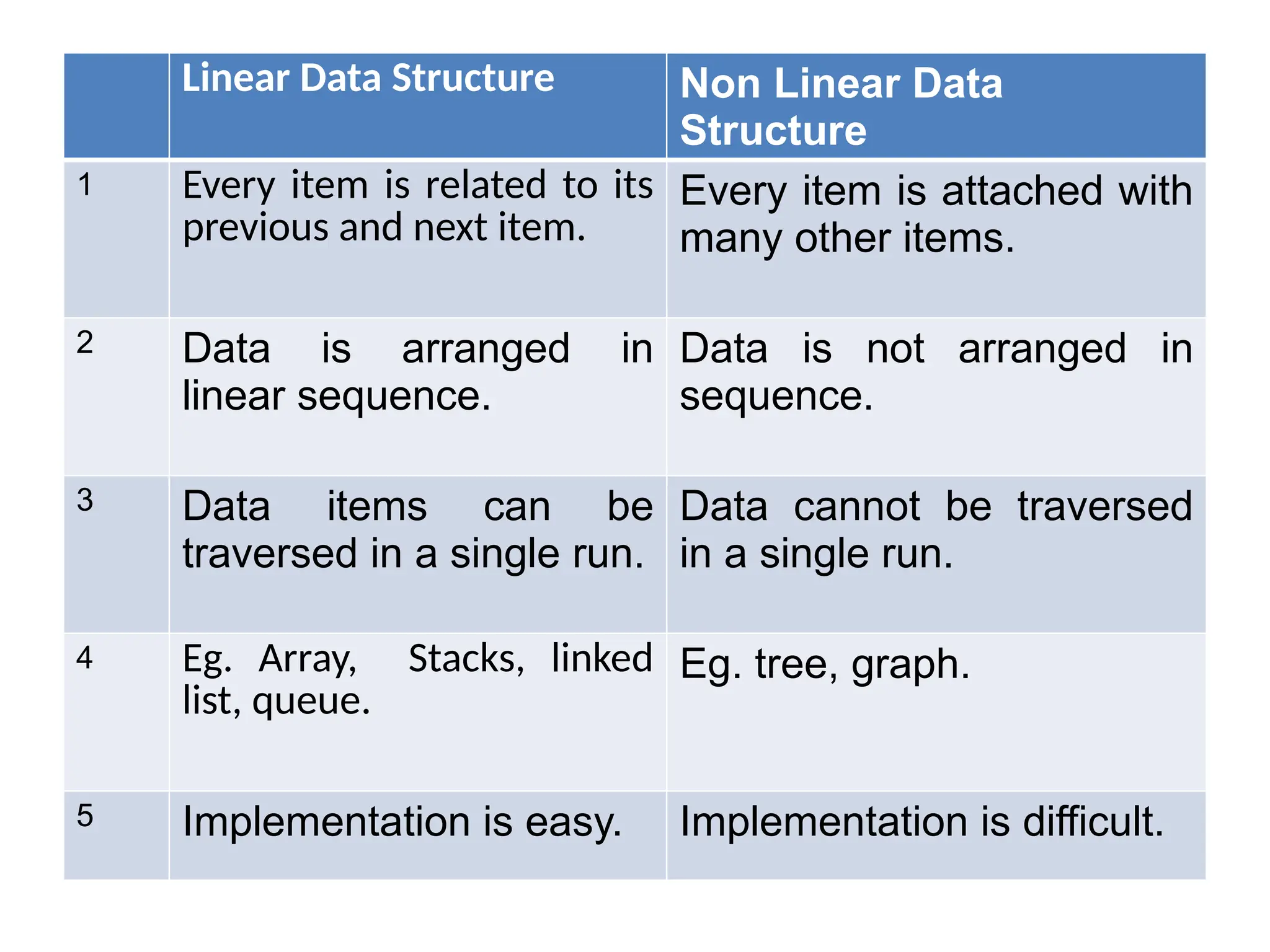
Linear Data StructureNon Linear Data
Structure
1 Every item is related to its
previous and next item.
Every item is attached with
many other items.
2 Data is arranged in
linear sequence.
Data is not arranged in
sequence.
3 Data items can be
traversed in a single run.
Data cannot be traversed
in a single run.
4 Eg. Array, Stacks, linked
list, queue.
Eg. tree, graph.
5 Implementation is easy. Implementation is difficult.
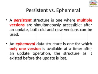
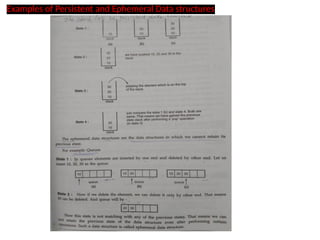
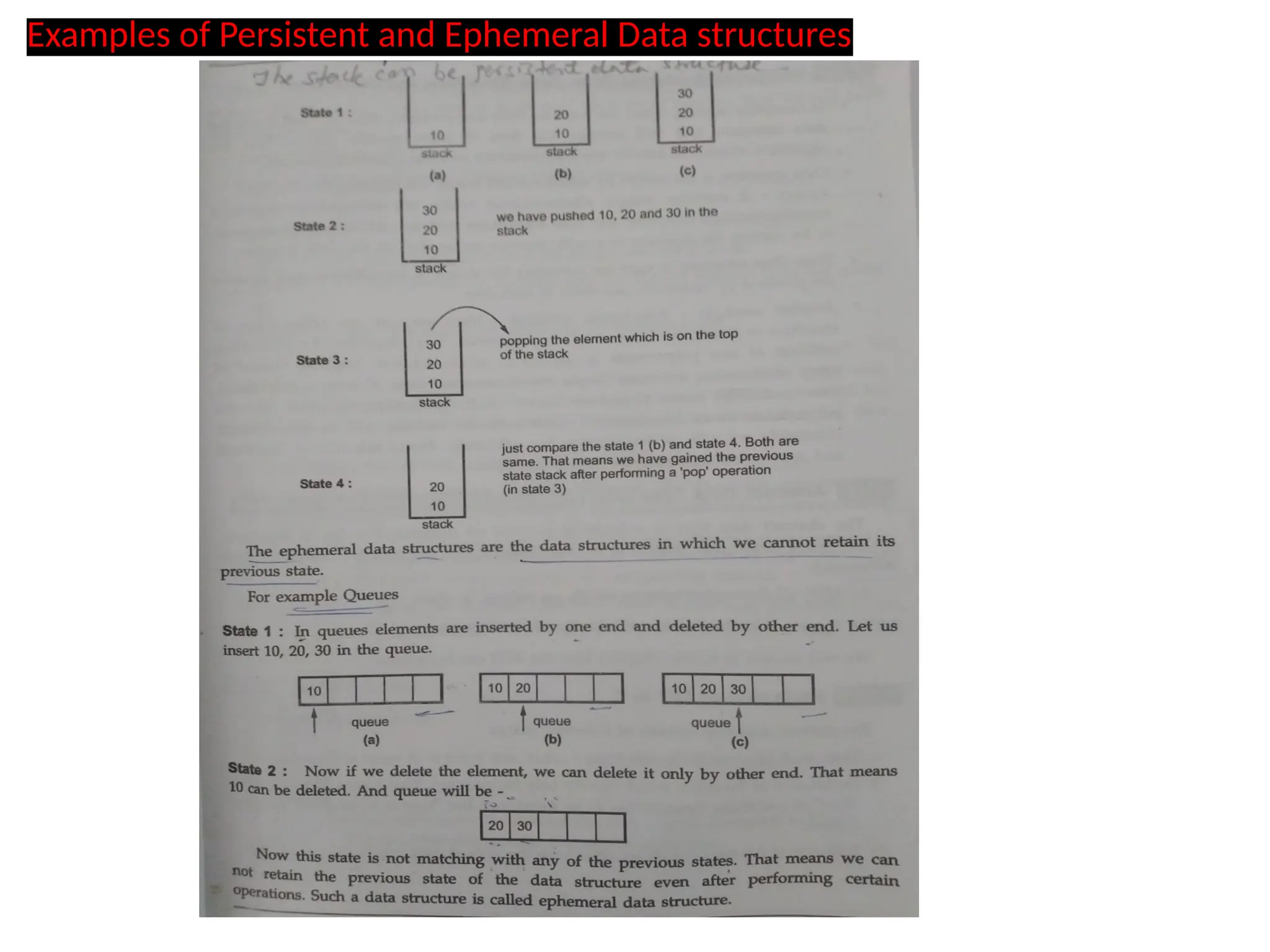
Persistent vs. Ephemeral
•A persistent structure is one where multiple
versions are simultaneously accessible: after
an update, both old and new versions can be
used.
• An ephemeral data structure is one for which
only one version is available at a time: after
an update operation, the structure as it
existed before the update is lost.
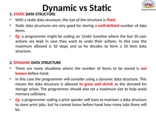
Dynamic vs Static
1.STATIC DATA STRUCTURE
• With a static data structure, the size of the structure is fixed.
• Static data structures are very good for storing a well-defined number of data
items.
• Eg: a programmer might be coding an 'Undo' function where the last 10 user
actions are kept in case they want to undo their actions. In this case the
maximum allowed is 10 steps and so he decides to form a 10 item data
structure.
2. DYNAMIC DATA STRUCTURE
• There are many situations where the number of items to be stored is not
known before hand.
• In this case the programmer will consider using a dynamic data structure. This
means the data structure is allowed to grow and shrink as the demand for
storage arises. The programmer should also set a maximum size to help avoid
memory collisions.
• Eg: a programmer coding a print spooler will have to maintain a data structure
to store print jobs, but he cannot know before hand how many jobs there will
be.
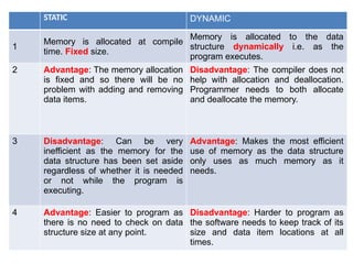
25.
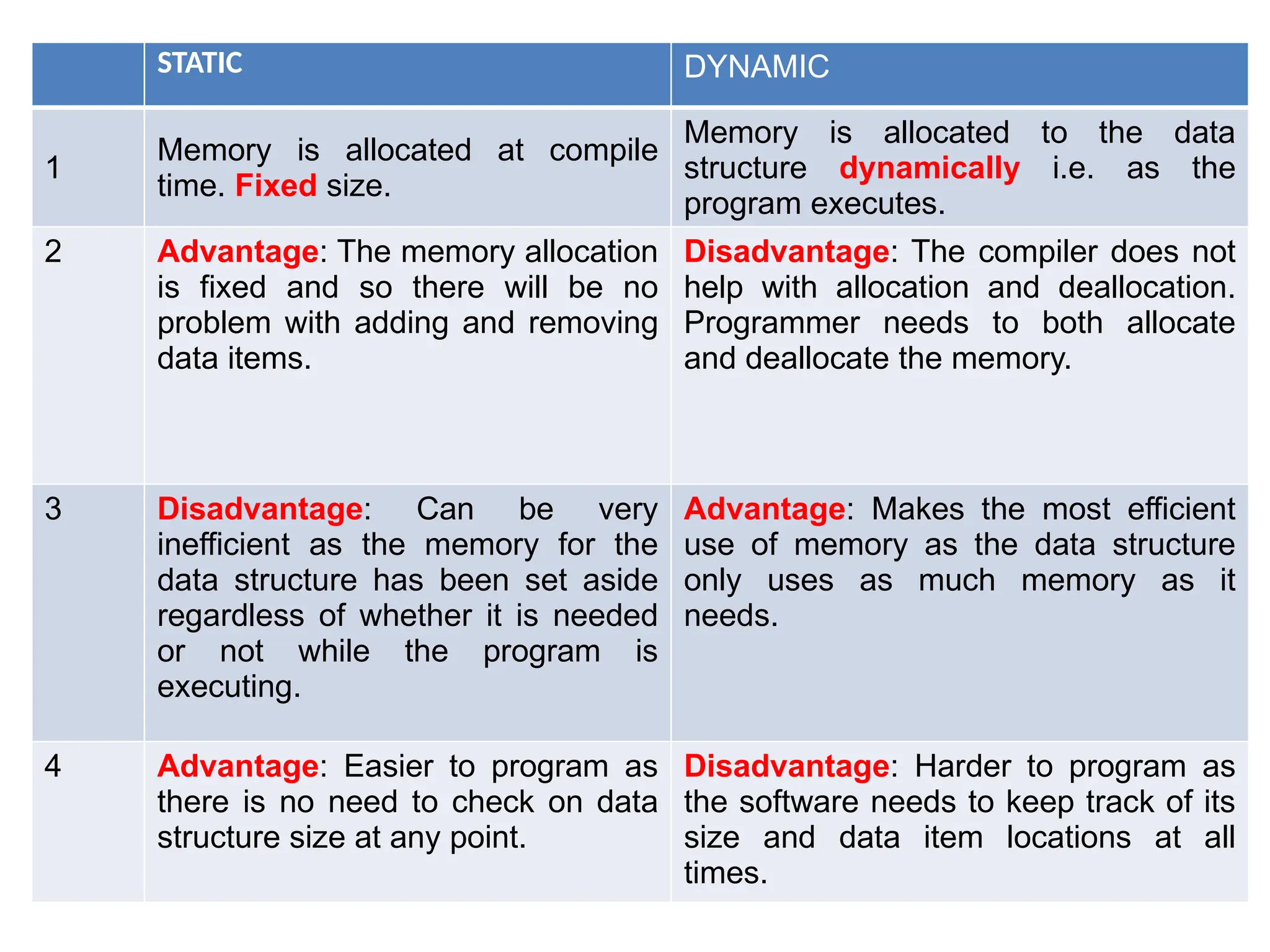
STATIC DYNAMIC
1
Memory isallocated at compile
time. Fixed size.
Memory is allocated to the data
structure dynamically i.e. as the
program executes.
2 Advantage: The memory allocation
is fixed and so there will be no
problem with adding and removing
data items.
Disadvantage: The compiler does not
help with allocation and deallocation.
Programmer needs to both allocate
and deallocate the memory.
3 Disadvantage: Can be very
inefficient as the memory for the
data structure has been set aside
regardless of whether it is needed
or not while the program is
executing.
Advantage: Makes the most efficient
use of memory as the data structure
only uses as much memory as it
needs.
4 Advantage: Easier to program as
there is no need to check on data
structure size at any point.
Disadvantage: Harder to program as
the software needs to keep track of its
size and data item locations at all
times.
26.
Algorithm
• An Algorithmis a finite sequence of
instructions, each of which has a clear
meaning and can be performed with a finite
amount of effort in a finite length of time.
• No matter what the input values may be, an
algorithm terminates after executing a finite
number of instructions.
27.
• In additionevery algorithm must satisfy the following criteria:
(Properties of Algorithm)
• Input: there are zero or more quantities, which are externally
supplied;
• Output: at least one quantity is produced;
• Definiteness: each instruction must be clear and unambiguous;
• Finiteness: if we trace out the instructions of an algorithm, then
for all cases the algorithm will terminate after a finite number of
steps;
• Effectiveness: every instruction must be sufficiently basic that it
can in principle be carried out by a person using only pencil and
paper. It is not enough that each operation be definite, but it must
also be feasible.
28.
• In formalcomputer science, one distinguishes
between an algorithm, and a program. A program
does not necessarily satisfy the fourth condition
(Finiteness).
• Example of such a program for a computer is its
operating system, which never terminates
(except for system crashes) but continues in a
wait loop until more jobs are entered.
• We represent algorithm using a pseudo language
that is a combination of the constructs of a
programming language together with informal
English statements.
29.
Designing Software WithFlowcharts And
Pseudo-code
In this section you will learn two
different ways of laying out a computer
algorithm independent of programming
language
30.
A Model ForCreating Computer Software
•Specify the problem
•Develop a design (algorithm)
•Implement the design
•Maintain the design
31.
What Is AnAlgorithm?
•The steps needed to solve a problem
•Characteristics
– Specific
– Unambiguous
– Language independent
32.
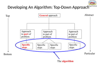
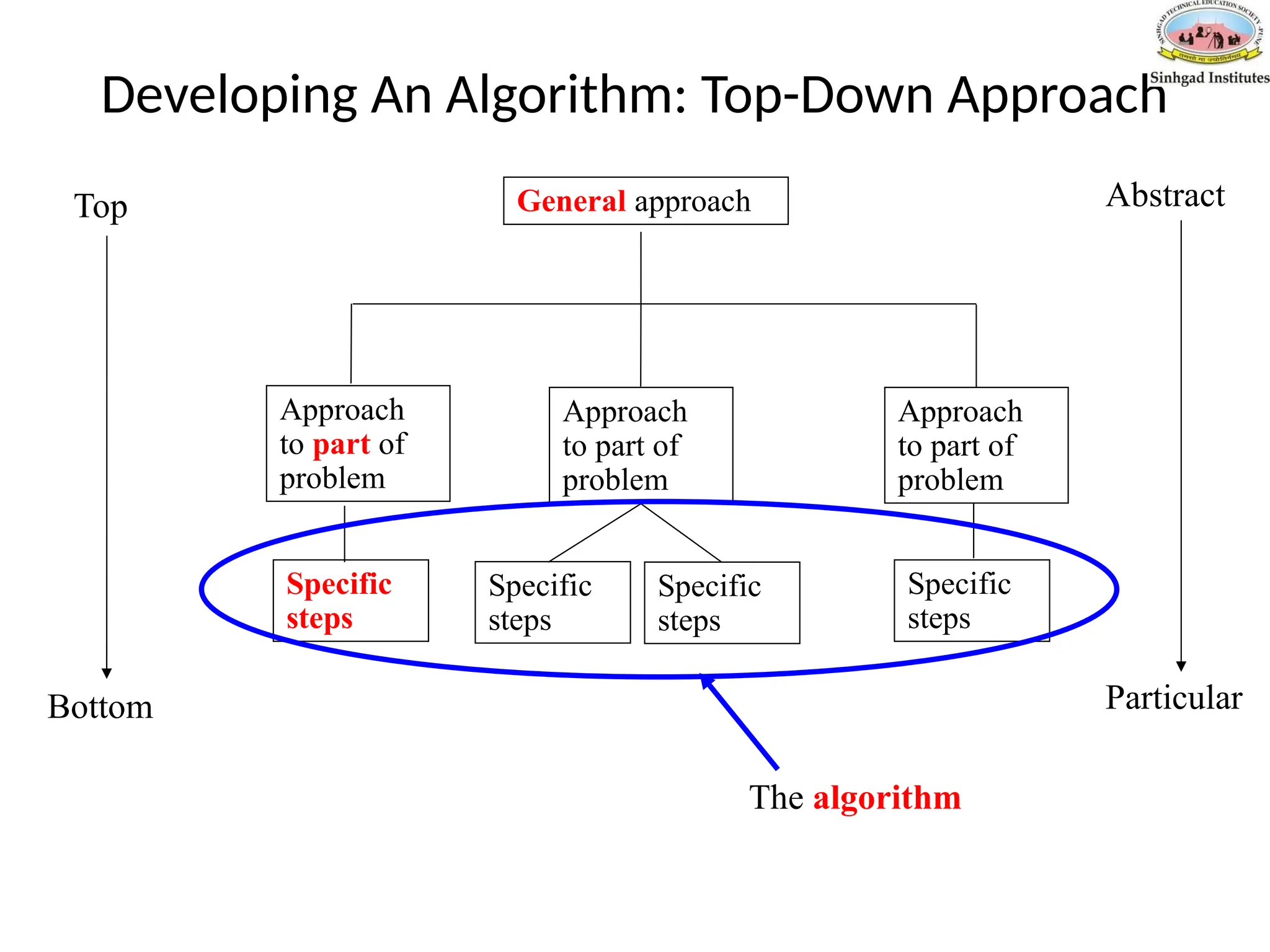
Developing An Algorithm:Top-Down Approach
General approach
Approach
to part of
problem
Specific
steps
Specific
steps
Specific
steps
Specific
steps
Approach
to part of
problem
Approach
to part of
problem
Abstract
Particular
Top
Bottom
The algorithm
Pseudo-Code
• Pseudo-Code isnothing but an informal way of
writing a program.
•No standard format (language independent)
35.
Pseudo-Code Statements
• Output
•Input
• Process
• Decision
• Repetition
Statements are carried out in order
Example: calling up a friend
1) Look up telephone number
2) Enter telephone number
3) Wait for someone to answer
: :
Pseudo-Code: Input
•Used toget information
•Information is stored in a variable
•General format:
• Input: Name of variable
•Example:
• Input user_name
38.
Pseudo-Code: Process
•For computerprograms it's usually an
assignment statement (sets a variable to some
value)
•General form:
•Variable=arithmetic expression
•Example:
•x = 2
•x =x + 1
•a =b * c
39.
Pseudo-Code: Decision Making
•If-then
•General form:
if (condition is met) then
statement(s)
• Example:
if temperature < 0 then
wear a jacket
If-then-else
General form:
if (condition is met) then
statement(s)
else
statements(s)
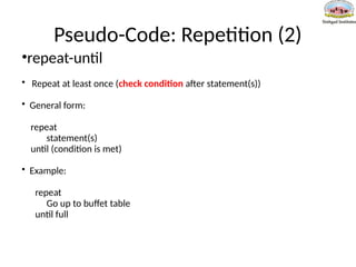
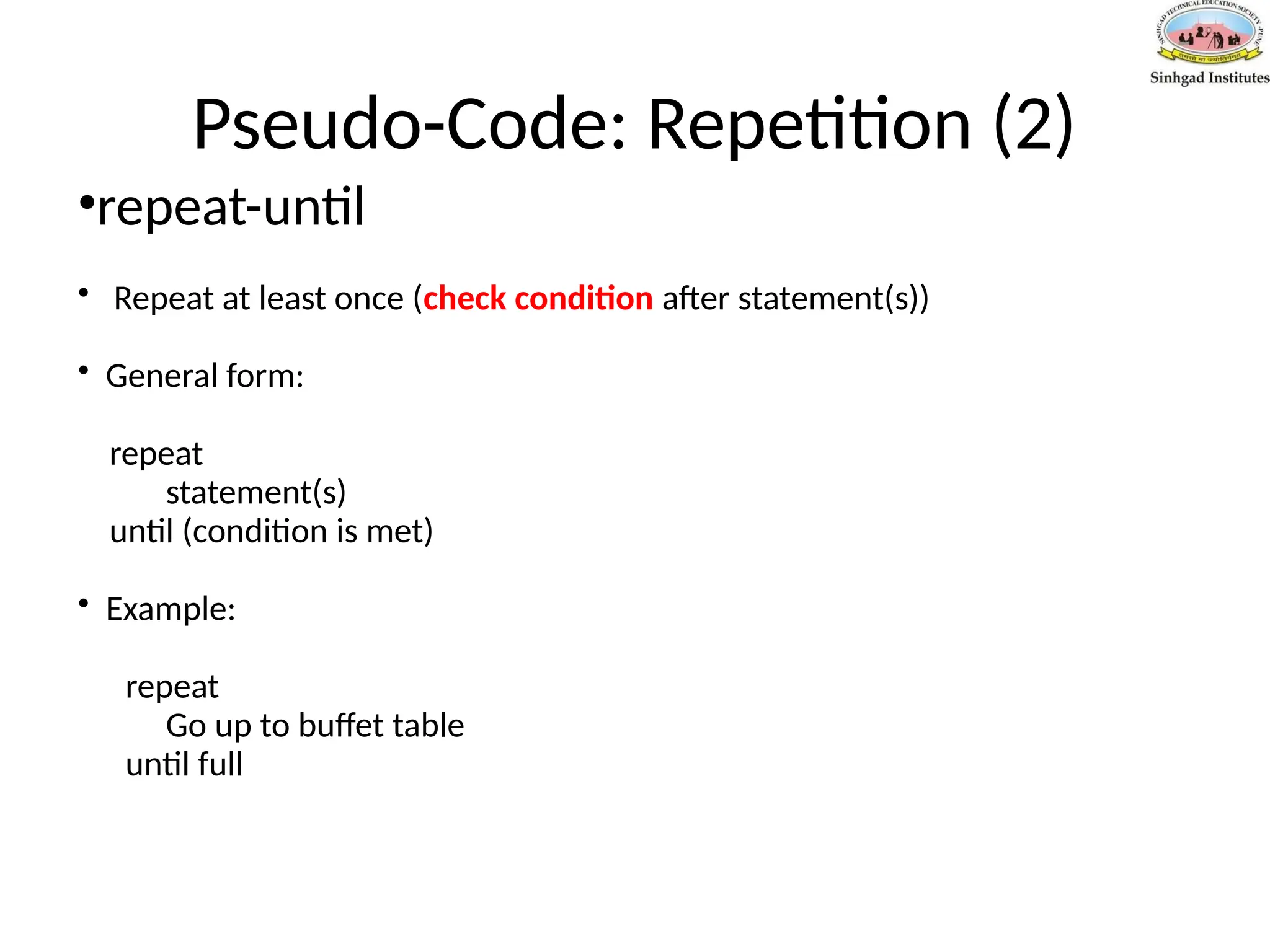
Pseudo-Code: Repetition (2)
•repeat-until
•Repeat at least once (check condition after statement(s))
• General form:
repeat
statement(s)
until (condition is met)
• Example:
repeat
Go up to buffet table
until full
43.
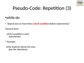
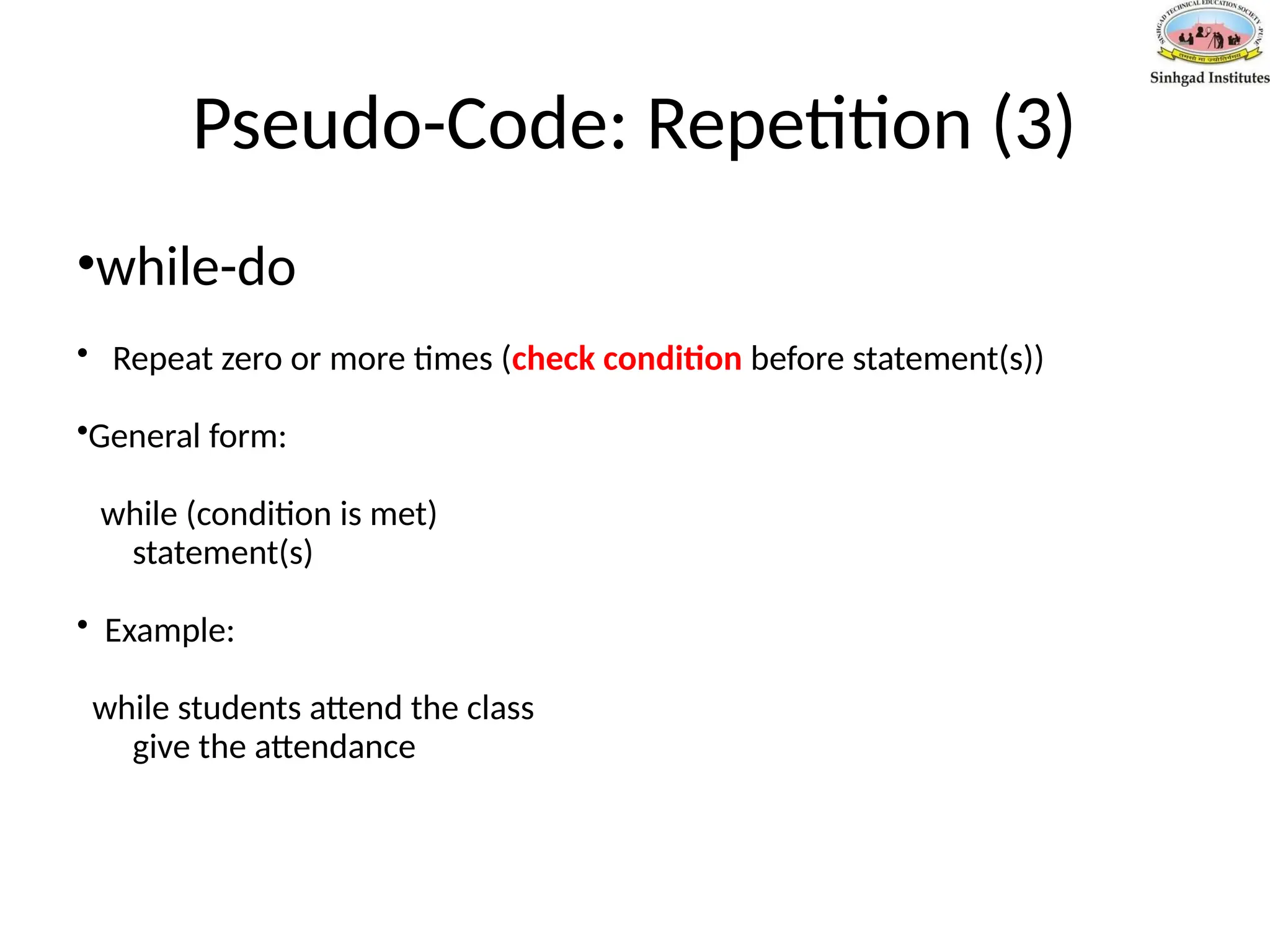
Pseudo-Code: Repetition (3)
•while-do
•Repeat zero or more times (check condition before statement(s))
•General form:
while (condition is met)
statement(s)
• Example:
while students attend the class
give the attendance
44.
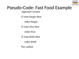
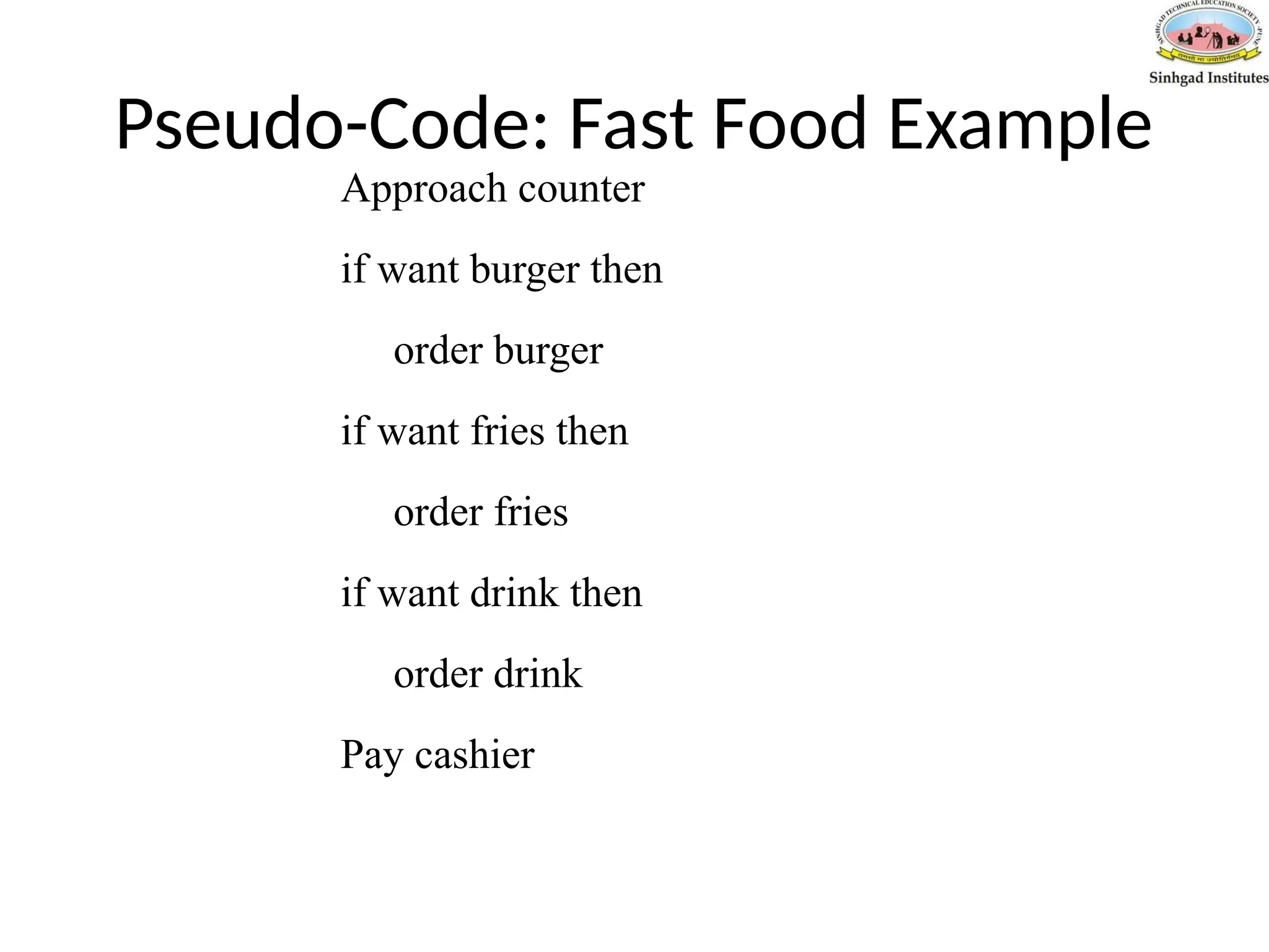
Pseudo-Code: Fast FoodExample
Approach counter
if want burger then
order burger
if want fries then
order fries
if want drink then
order drink
Pay cashier
45.
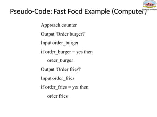
Pseudo-Code: Fast FoodExample (Computer)
Approach counter
Output 'Order burger?'
Input order_burger
if order_burger = yes then
order_burger
Output 'Order fries?'
Input order_fries
if order_fries = yes then
order fries
46.
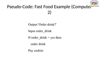
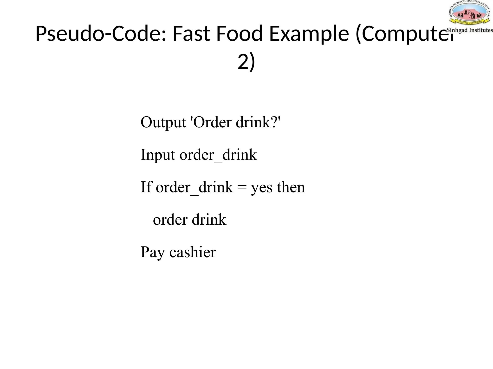
Pseudo-Code: Fast FoodExample (Computer
2)
Output 'Order drink?'
Input order_drink
If order_drink = yes then
order drink
Pay cashier
47.
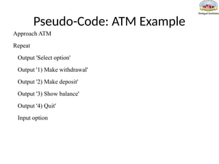
Pseudo-Code: ATM Example
•Usepseudo-code to specify the algorithm for an ATM bank machine. The
bank machine has four options: 1) Show current balance 2) Deposit money 3)
Withdraw money 4) Quit. After an option has been selected, the ATM will
continue displaying the four options to the person until he selects the option
to quit the ATM.
48.
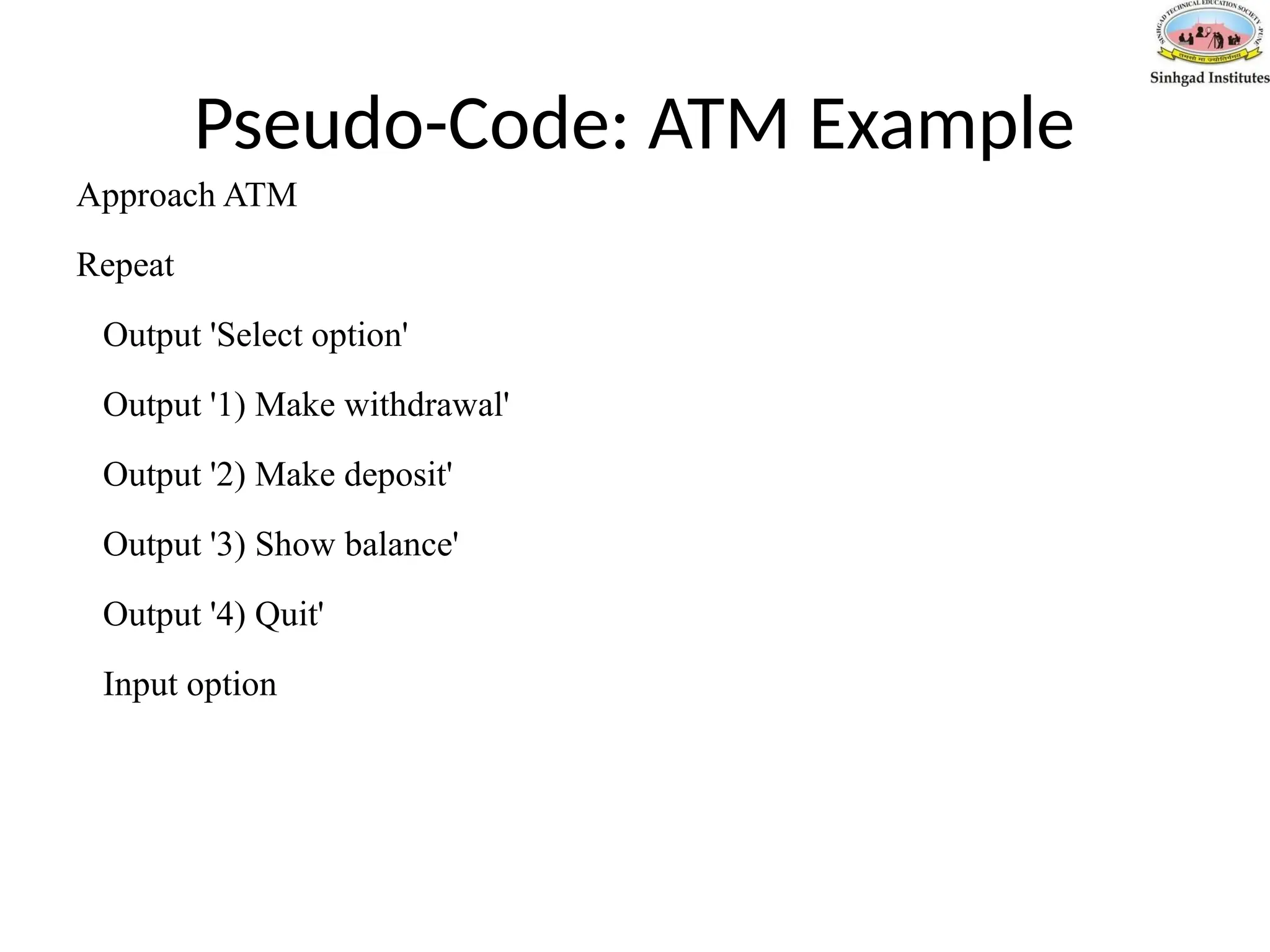
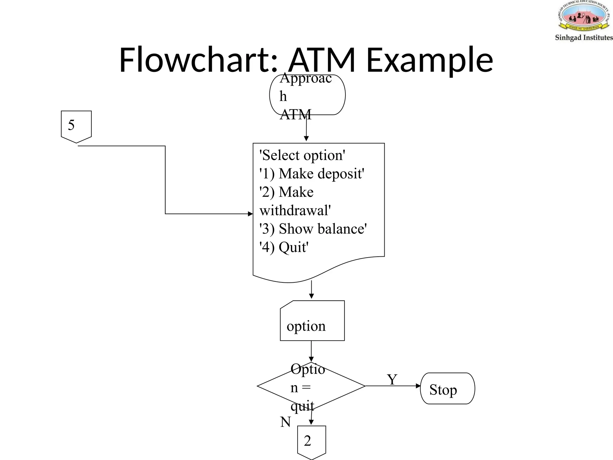
Pseudo-Code: ATM Example
ApproachATM
Repeat
Output 'Select option'
Output '1) Make withdrawal'
Output '2) Make deposit'
Output '3) Show balance'
Output '4) Quit'
Input option
49.
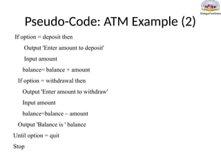
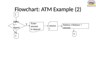
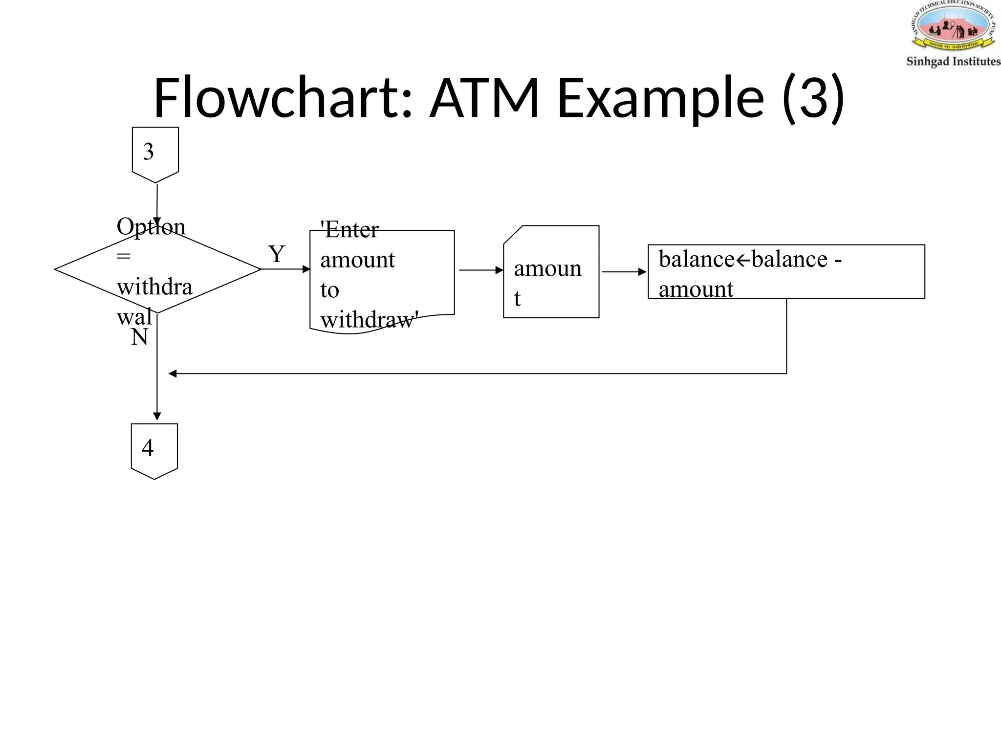
Pseudo-Code: ATM Example(2)
If option = deposit then
Output 'Enter amount to deposit'
Input amount
balance= balance + amount
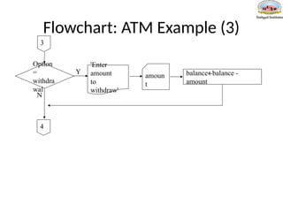
If option = withdrawal then
Output 'Enter amount to withdraw'
Input amount
balance=balance – amount
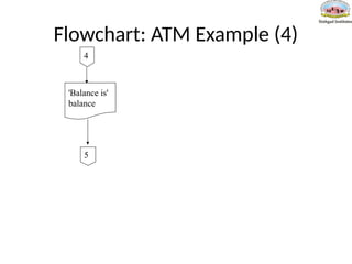
Output 'Balance is ' balance
Until option = quit
Stop
50.
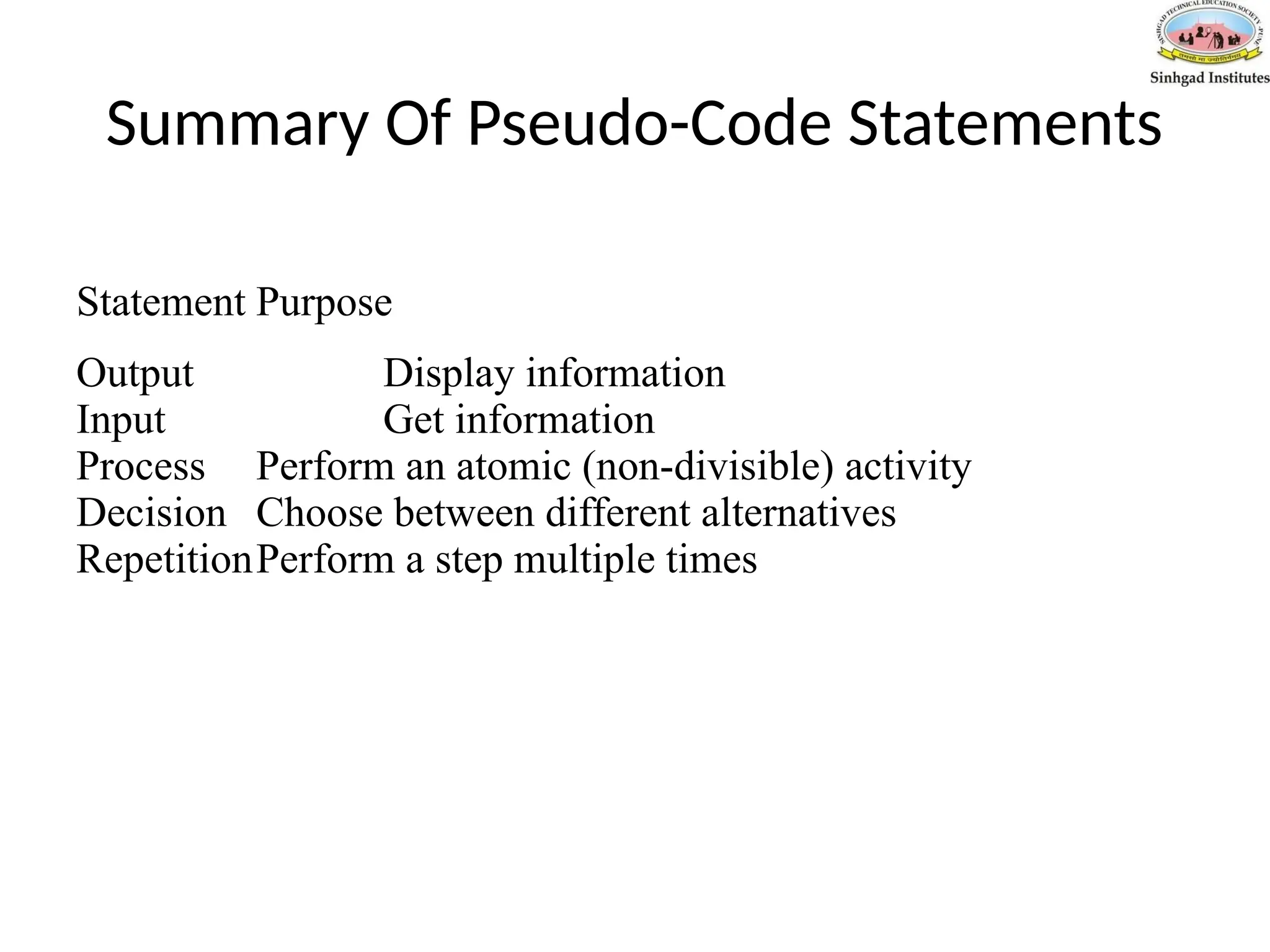
Summary Of Pseudo-CodeStatements
Statement Purpose
Output Display information
Input Get information
Process Perform an atomic (non-divisible) activity
Decision Choose between different alternatives
RepetitionPerform a step multiple times
Flowchart: Fast FoodExample
•Draw a flowchart to outline the algorithm for a person who ordering food at
a fast food restaurant. At the food counter, the person can either order not
order the following items: a burger, fries and a drink. After placing her order
the person then goes to the cashier.
53.
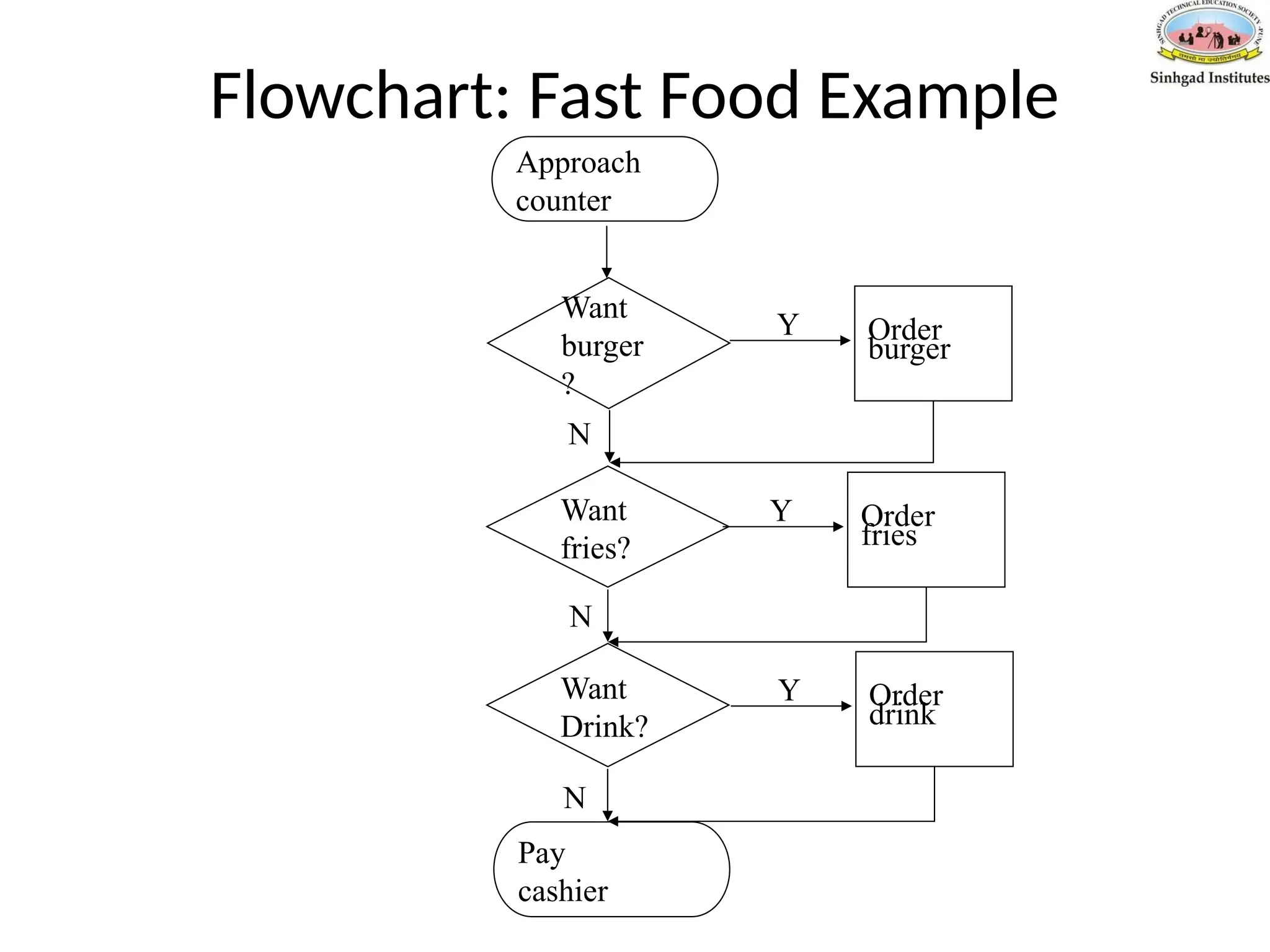
Flowchart: Fast FoodExample
Approach
counter
Want
burger
?
Want
fries?
Want
Drink?
Pay
cashier
Order
burger
Y
Order
fries
Y
Order
drink
Y
N
N
N
54.
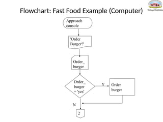
Flowchart: Fast FoodExample (Computer)
Approach
console
Order_
burger
= 'yes'
Order_
burger
'Order
Burger?'
Order
burger
Y
N
2
55.
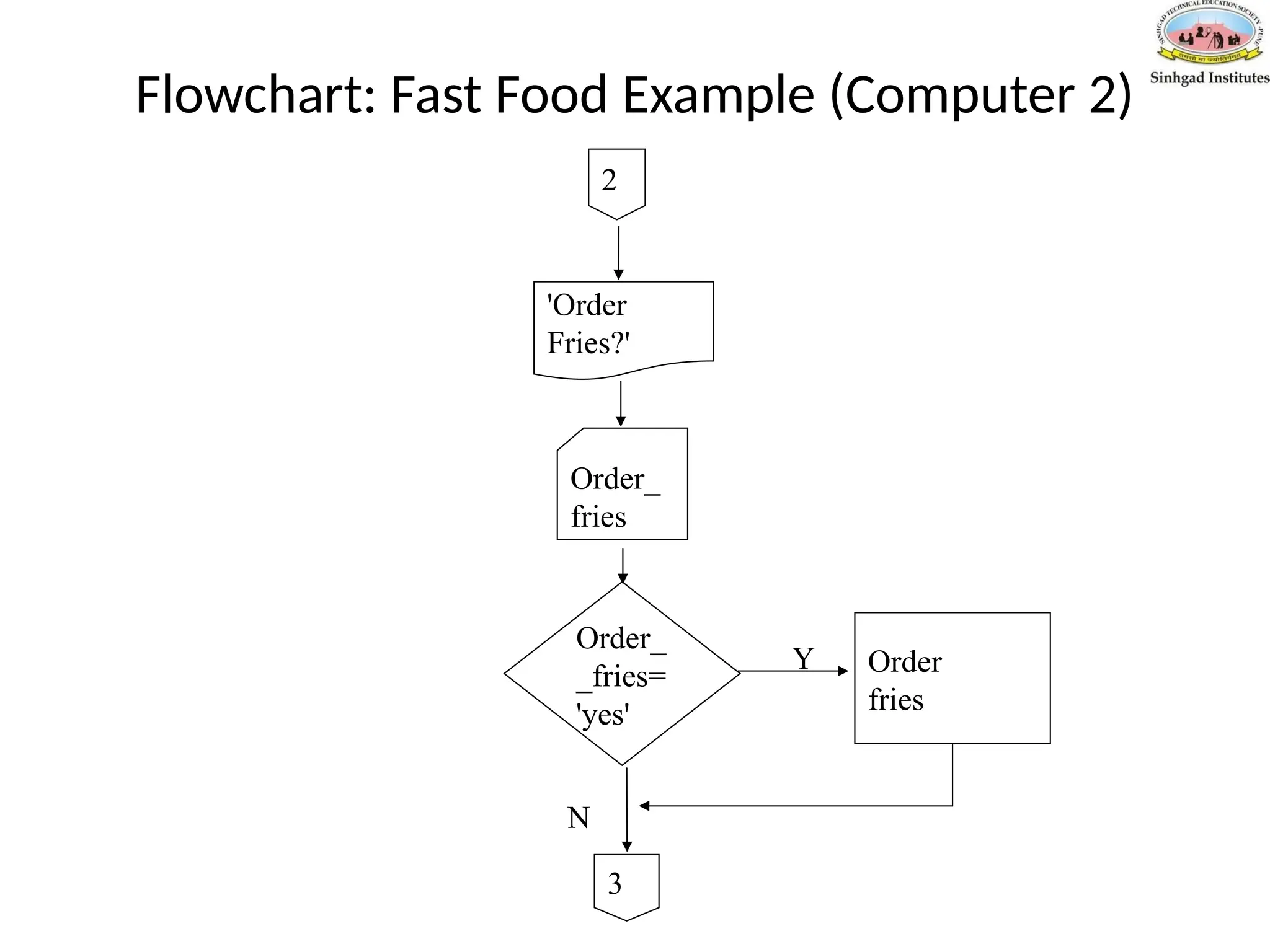
Flowchart: Fast FoodExample (Computer 2)
Order_
_fries=
'yes'
Order_
fries
'Order
Fries?'
Order
fries
Y
N
3
2
56.
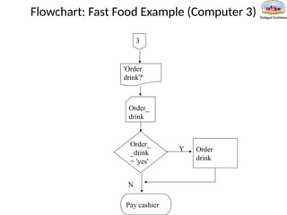
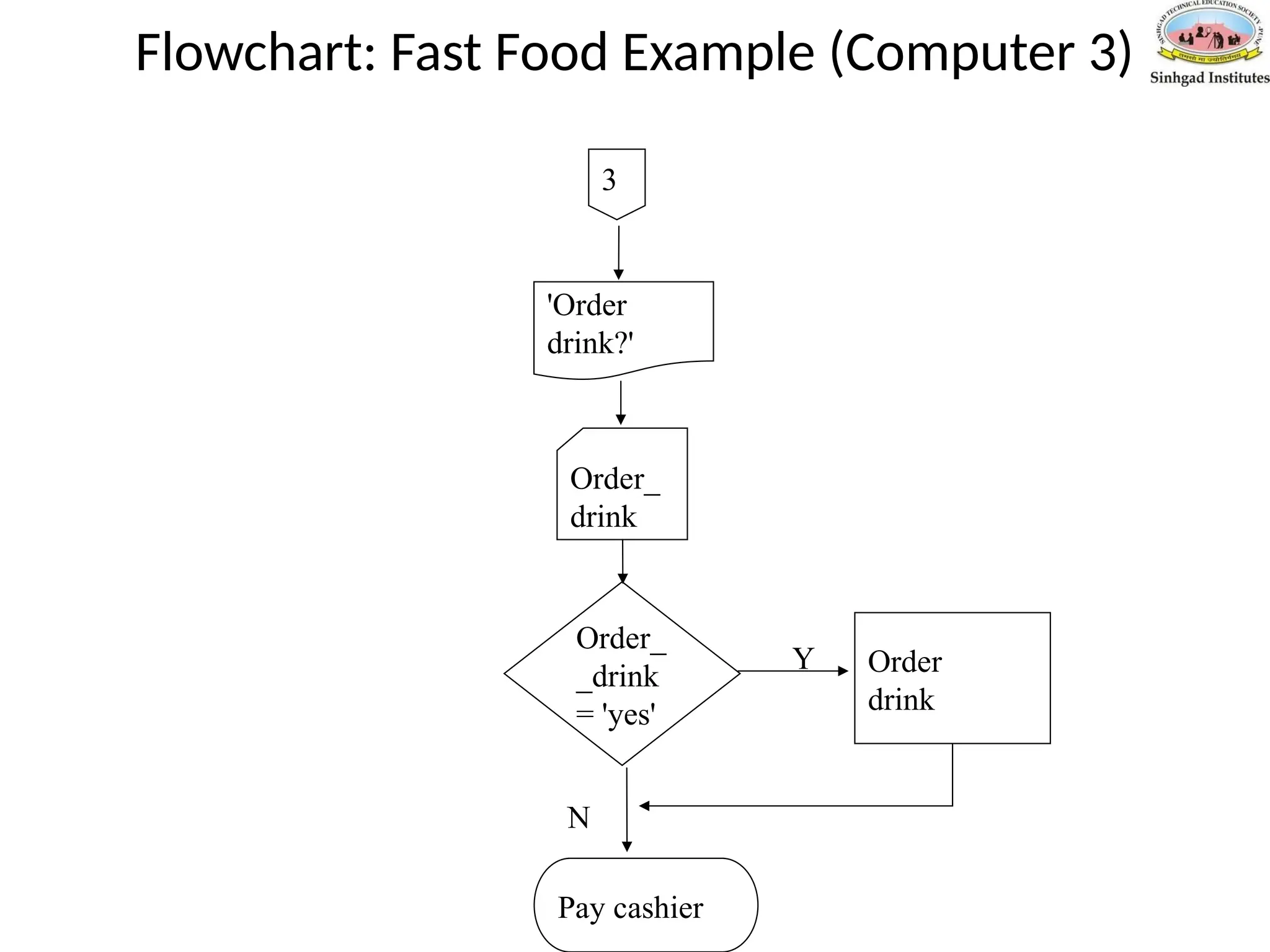
Flowchart: Fast FoodExample (Computer 3)
Order_
_drink
= 'yes'
Order_
drink
'Order
drink?'
Order
drink
Y
N
3
Pay cashier
57.
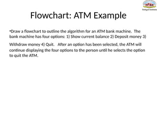
Flowchart: ATM Example
•Drawa flowchart to outline the algorithm for an ATM bank machine. The
bank machine has four options: 1) Show current balance 2) Deposit money 3)
Withdraw money 4) Quit. After an option has been selected, the ATM will
continue displaying the four options to the person until he selects the option
to quit the ATM.
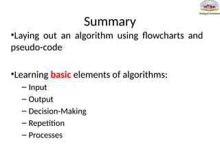
Summary
•Laying out analgorithm using flowcharts and
pseudo-code
•Learning basic elements of algorithms:
– Input
– Output
– Decision-Making
– Repetition
– Processes
63.
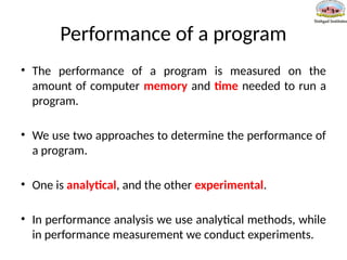
Performance of aprogram
• The performance of a program is measured on the
amount of computer memory and time needed to run a
program.
• We use two approaches to determine the performance of
a program.
• One is analytical, and the other experimental.
• In performance analysis we use analytical methods, while
in performance measurement we conduct experiments.
64.
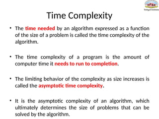
Time Complexity
• Thetime needed by an algorithm expressed as a function
of the size of a problem is called the time complexity of the
algorithm.
• The time complexity of a program is the amount of
computer time it needs to run to completion.
• The limiting behavior of the complexity as size increases is
called the asymptotic time complexity.
• It is the asymptotic complexity of an algorithm, which
ultimately determines the size of problems that can be
solved by the algorithm.
65.
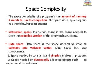
Space Complexity
• Thespace complexity of a program is the amount of memory
it needs to run to completion. The space need by a program
has the following components:
• Instruction space: Instruction space is the space needed to
store the compiled version of the program instructions.
• Data space: Data space is the space needed to store all
constant and variable values. Data space has two
components:
1. Space needed by constants and simple variables in program.
2. Space needed by dynamically allocated objects such as
arrays and class instances.
66.
Algorithm Design Goals
•The three basic design goals that one should strive for in a
program are:
1. Try to save Time
2. Try to save Space
3. Try to save Face
• A program that runs faster is a better program, so saving time is
an obvious goal.
• Like wise, a program that saves space over a competing program
is considered desirable.
• We want to “save face” by preventing the program from locking
up or generating reams of garbled data.
67.
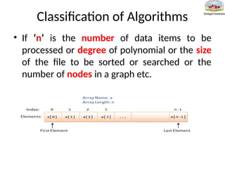
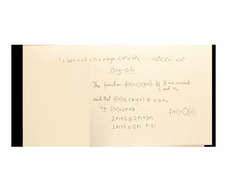
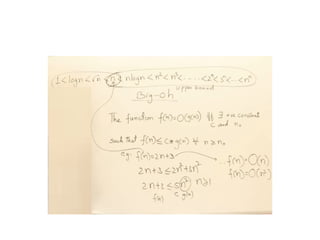
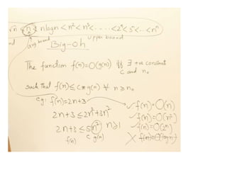
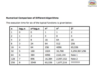
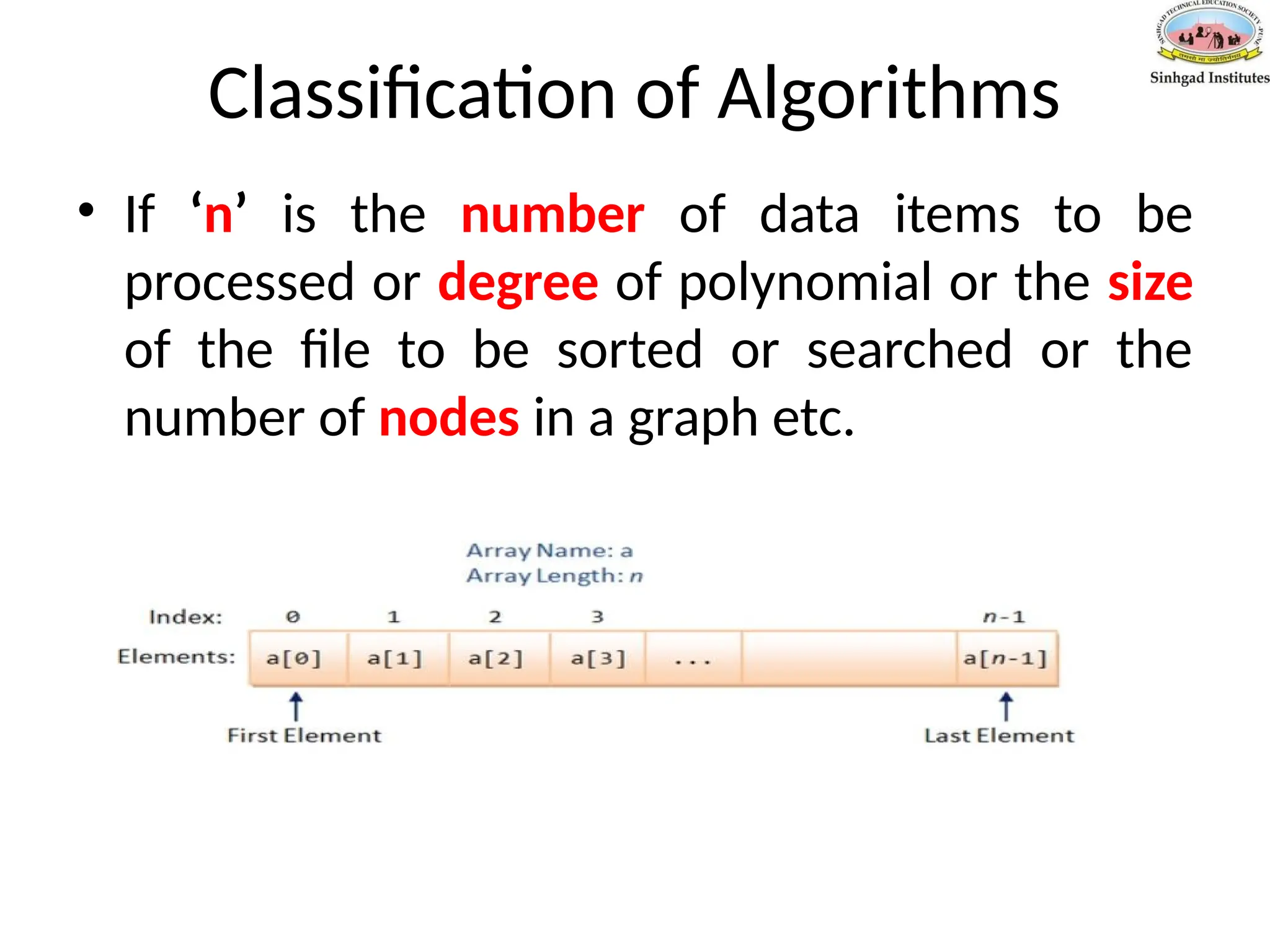
Classification of Algorithms
•If ‘n’ is the number of data items to be
processed or degree of polynomial or the size
of the file to be sorted or searched or the
number of nodes in a graph etc.
68.
• 1 -Next instructions of most programs are
executed once or at most only a few times.
If all the instructions of a program have
this property, we say that its running time is a
constant.
69.
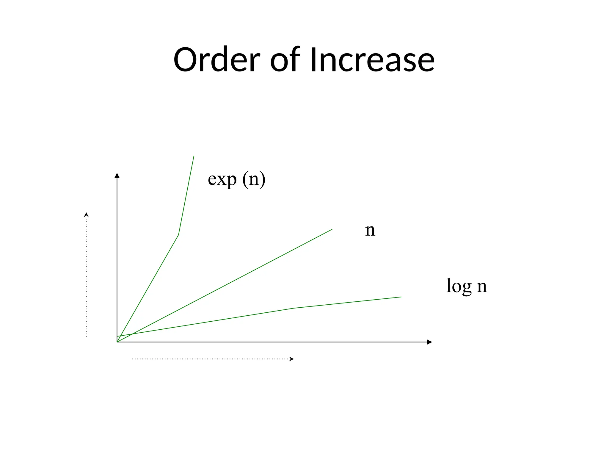
• Log n-When the running time of a program is
logarithmic, the program gets slightly slower
as n grows.
• This running time commonly occurs in
programs that solve a big problem by
transforming it into a smaller problem, cutting
the size by some constant fraction.,
70.
• n -Whenthe running time of a program is linear,
it is generally the case that a small amount of
processing is done on each input element.
– This is the optimal situation for an algorithm that
must process n inputs.
• n. log n -This running time arises for algorithms
that solve a problem by breaking it up into
smaller sub-problems, solving then
independently, and then combining the
solutions.
-When n doubles, the running time more
than doubles.
71.
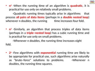
• n2
-When therunning time of an algorithm is quadratic, it is
practical for use only on relatively small problems.
-Quadratic running times typically arise in algorithms that
process all pairs of data items (perhaps in a double nested loop)
whenever n doubles, the running time increases four fold.
• n3
-Similarly, an algorithm that process triples of data items
(perhaps in a triple–nested loop) has a cubic running time and
is practical for use only on small problems.
-Whenever n doubles, the running time increases eight
fold.
• 2n
-Few algorithms with exponential running time are likely to
be appropriate for practical use, such algorithms arise naturally
as “brute–force” solutions to problems. -Whenever n
doubles, the running time squares.
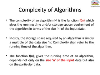
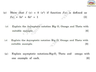
Complexity of Algorithms
•The complexity of an algorithm M is the function f(n) which
gives the running time and/or storage space requirement of
the algorithm in terms of the size ‘n’ of the input data.
• Mostly, the storage space required by an algorithm is simply
a multiple of the data size ‘n’. Complexity shall refer to the
running time of the algorithm.
• The function f(n), gives the running time of an algorithm,
depends not only on the size ‘n’ of the input data but also
on the particular data.
80.
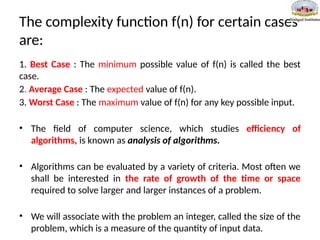
The complexity functionf(n) for certain cases
are:
1. Best Case : The minimum possible value of f(n) is called the best
case.
2. Average Case : The expected value of f(n).
3. Worst Case : The maximum value of f(n) for any key possible input.
• The field of computer science, which studies efficiency of
algorithms, is known as analysis of algorithms.
• Algorithms can be evaluated by a variety of criteria. Most often we
shall be interested in the rate of growth of the time or space
required to solve larger and larger instances of a problem.
• We will associate with the problem an integer, called the size of the
problem, which is a measure of the quantity of input data.
81.
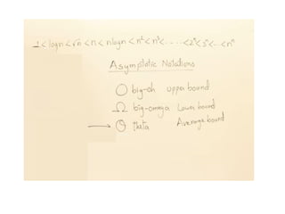
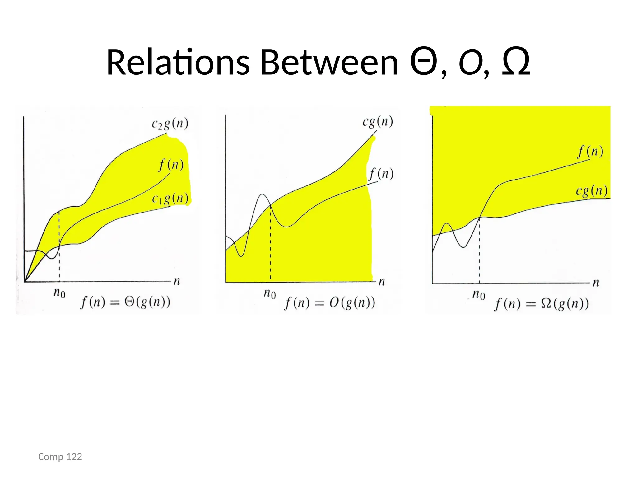
Rate of Growth
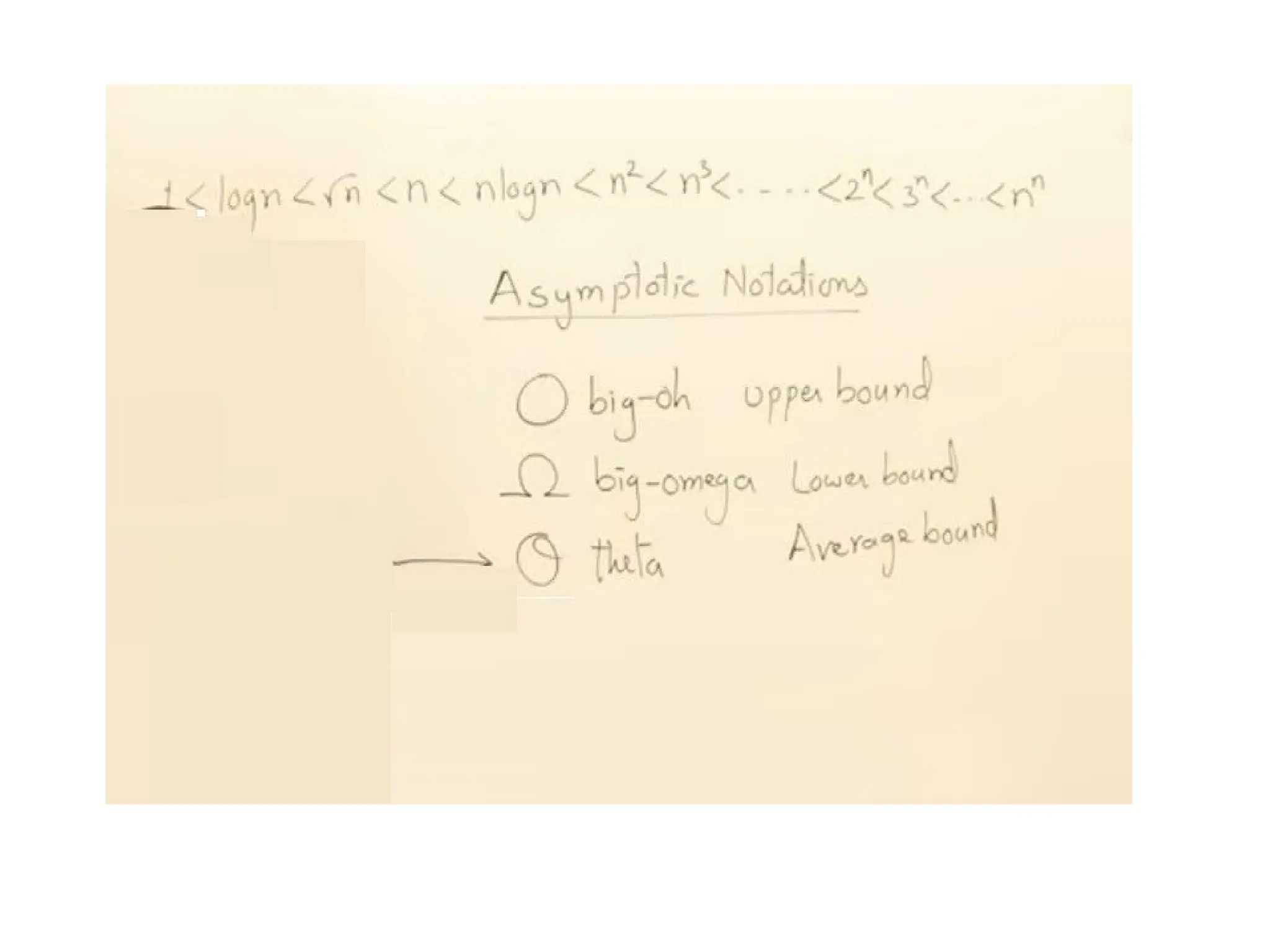
•The following notations are commonly use
notations in performance analysis and used to
characterize the complexity of an algorithm:
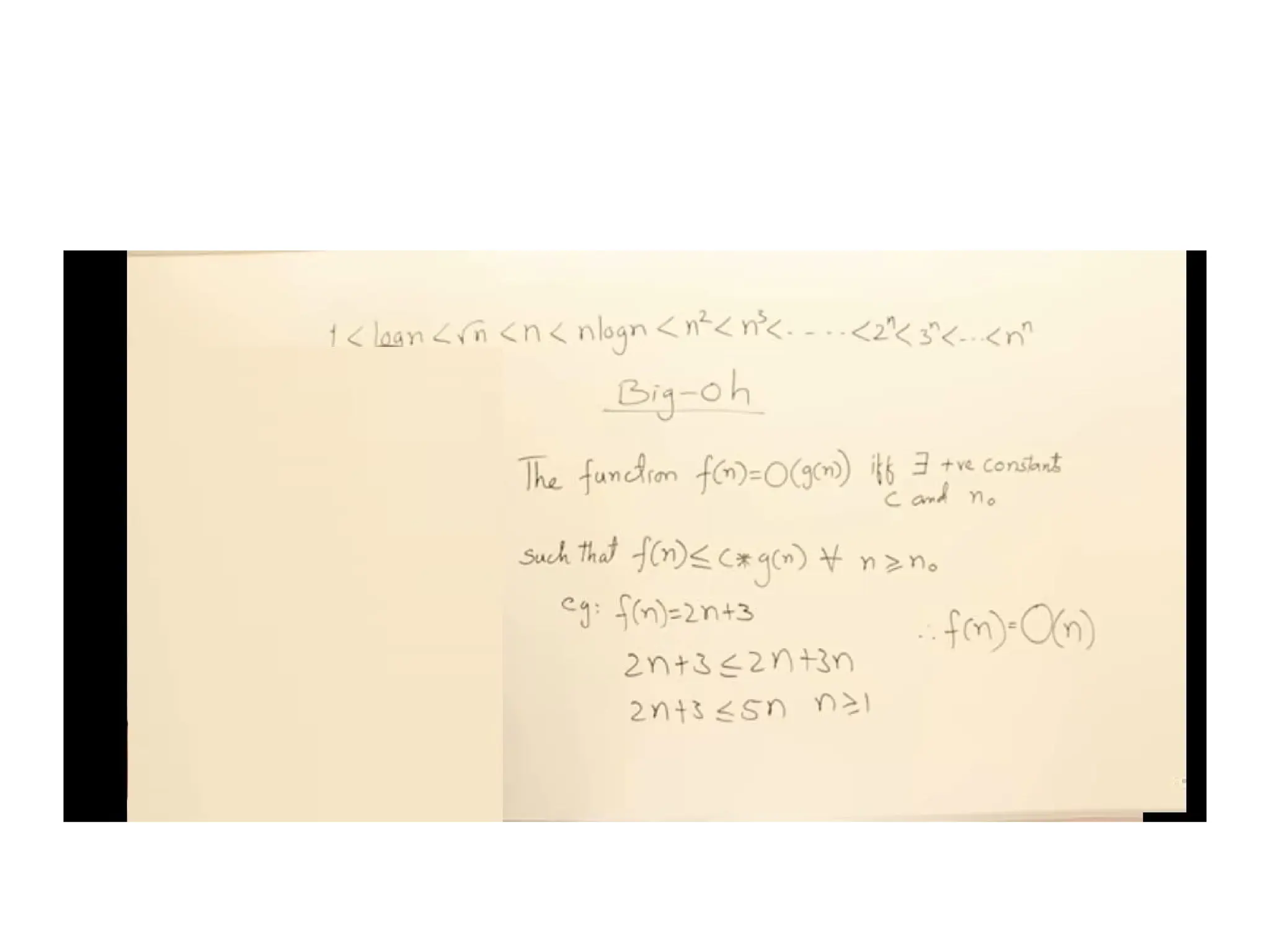
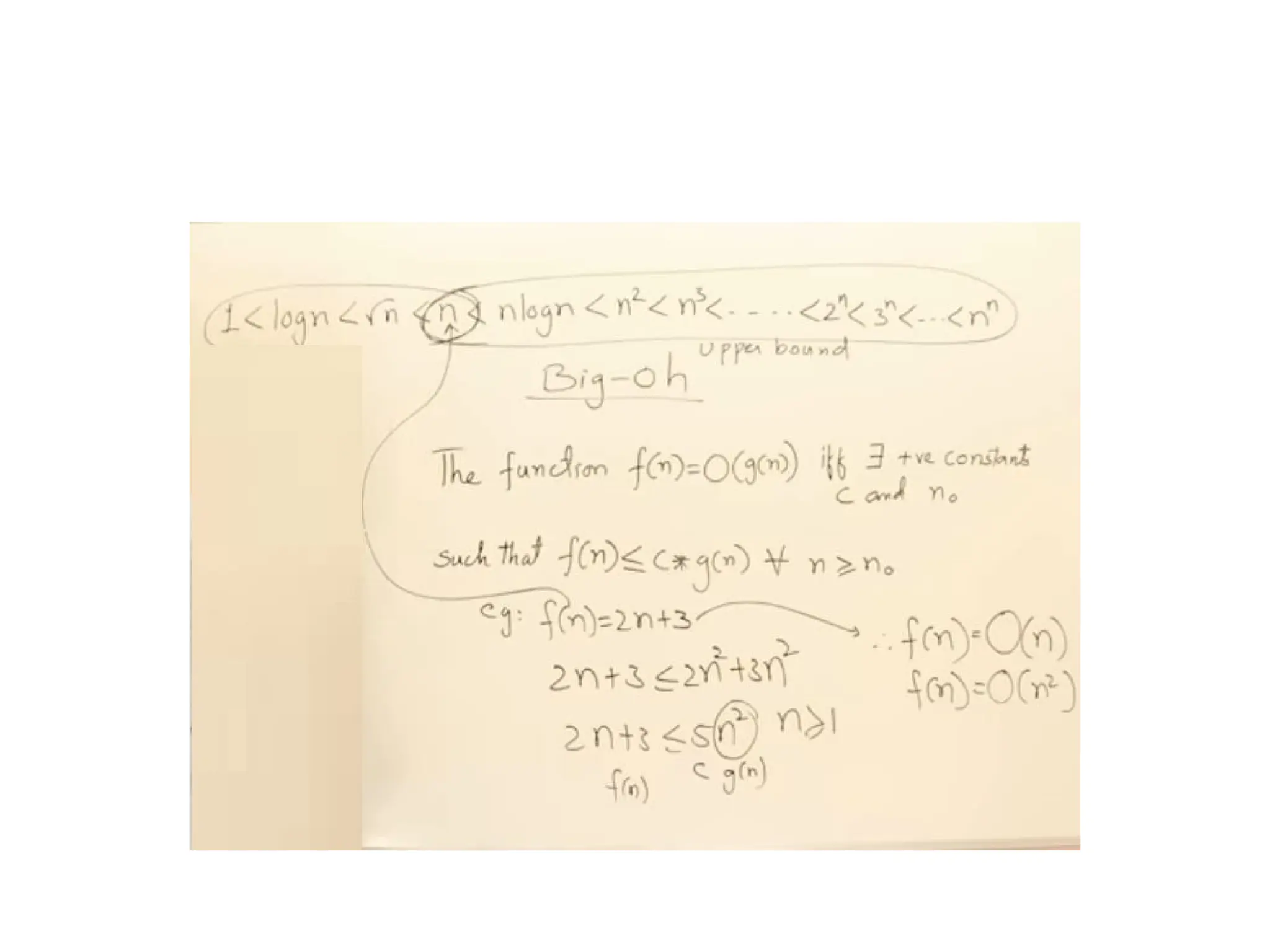
• 1. Big–OH (O) ,
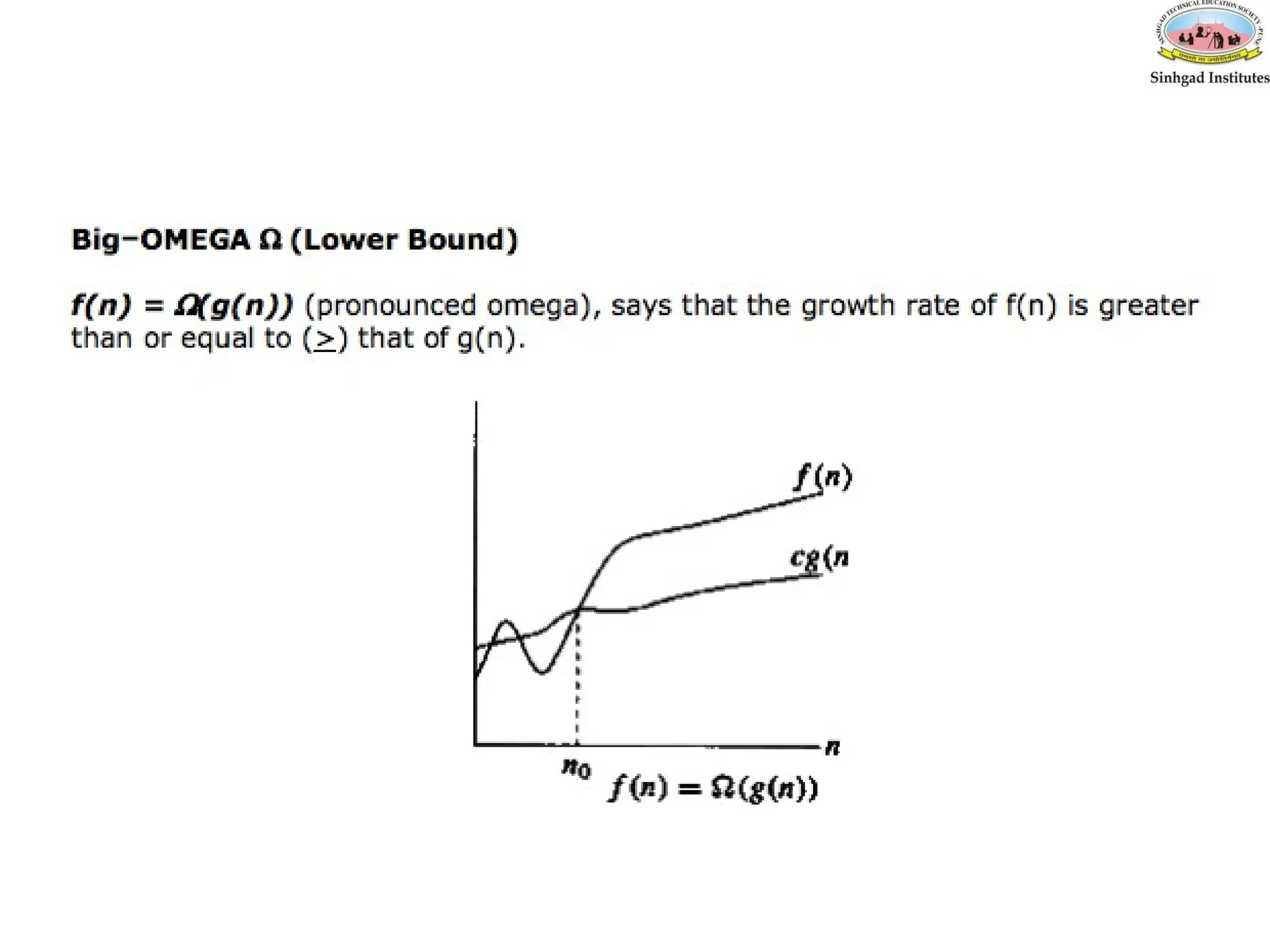
• 2. Big–OMEGA (Ω),
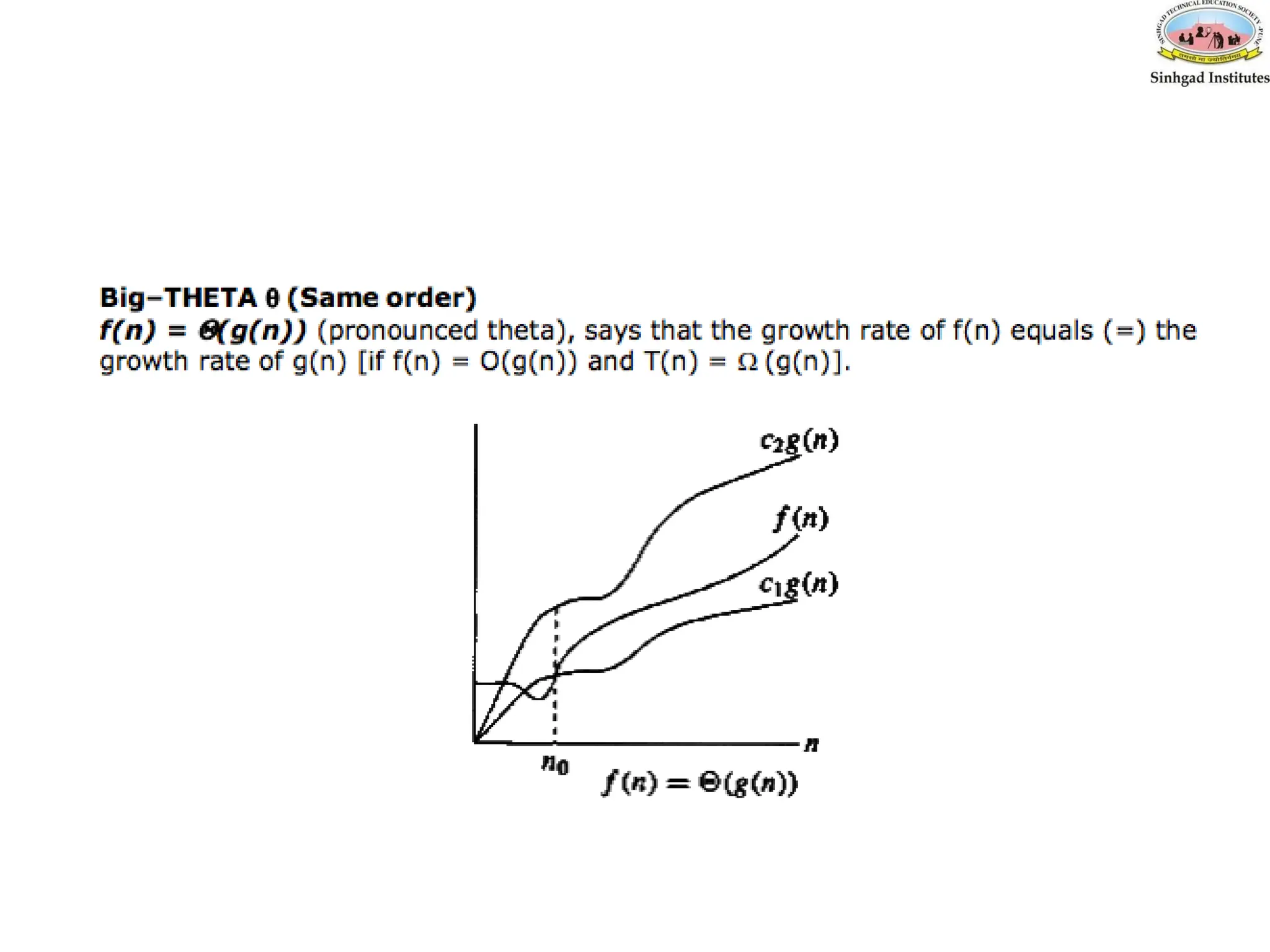
• 3. Big–THETA (θ)
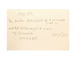
83.
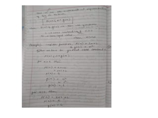
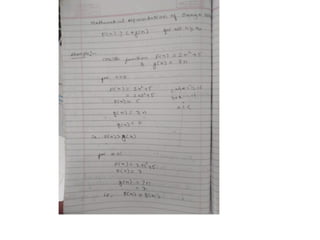
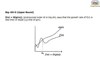
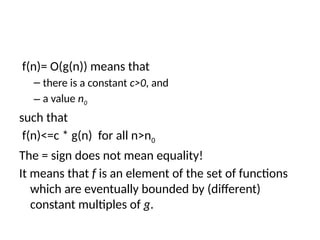
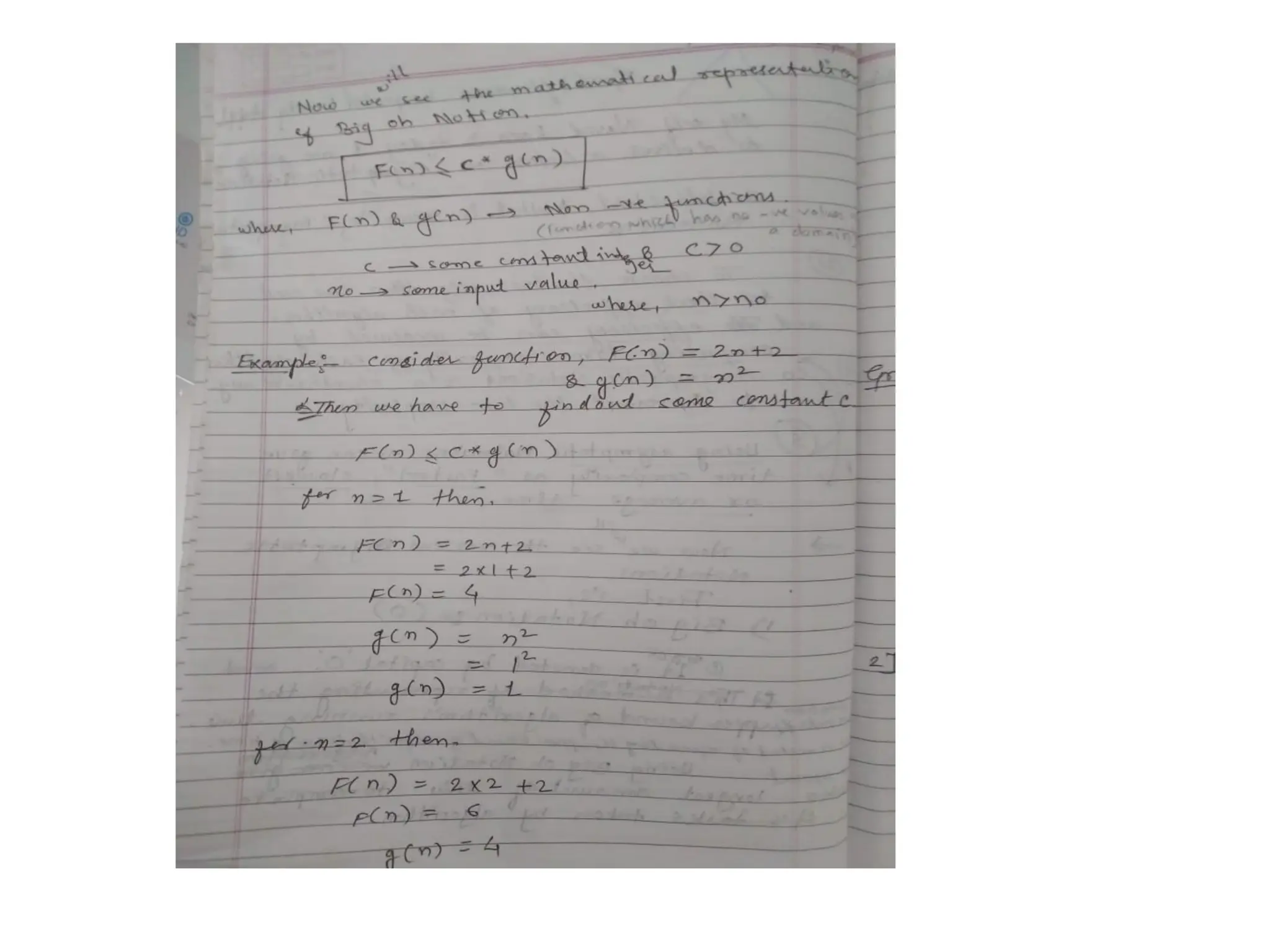
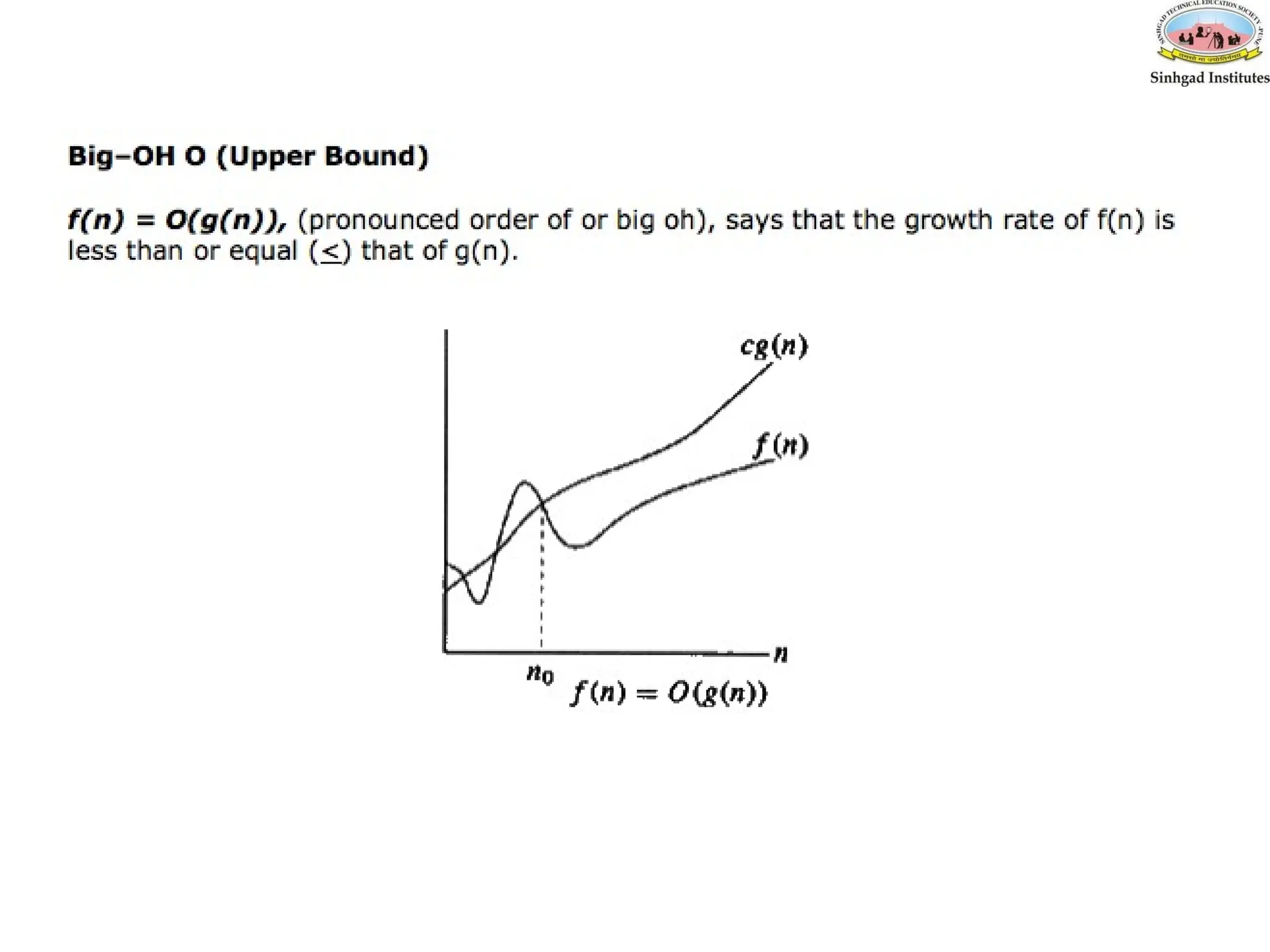
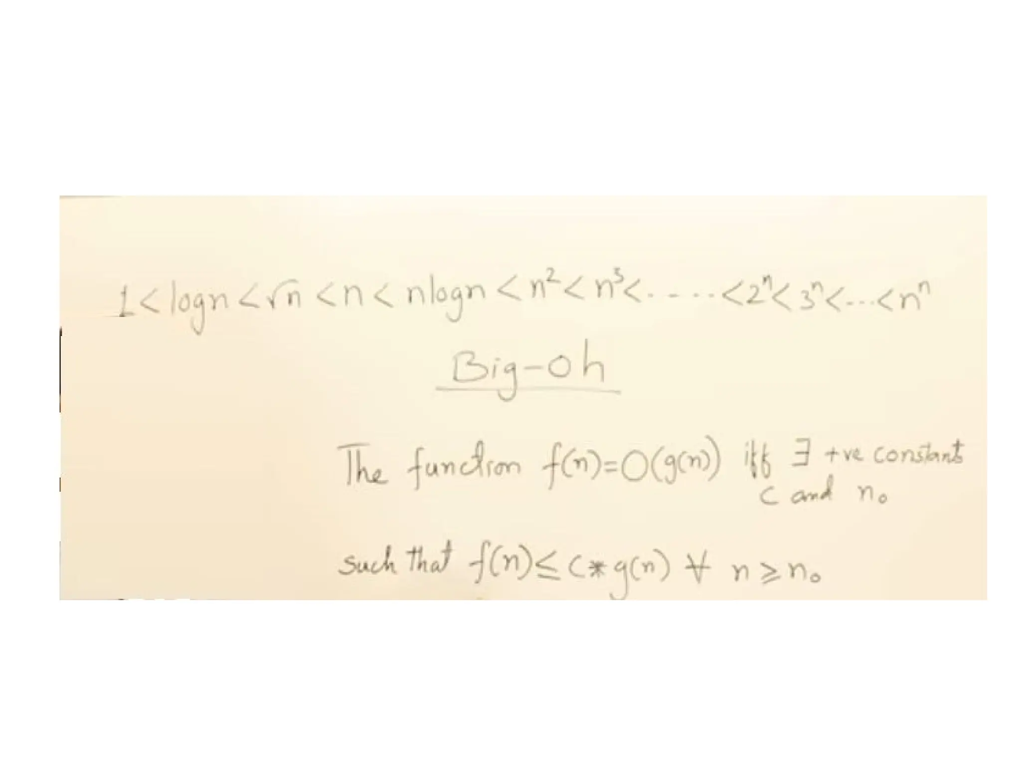
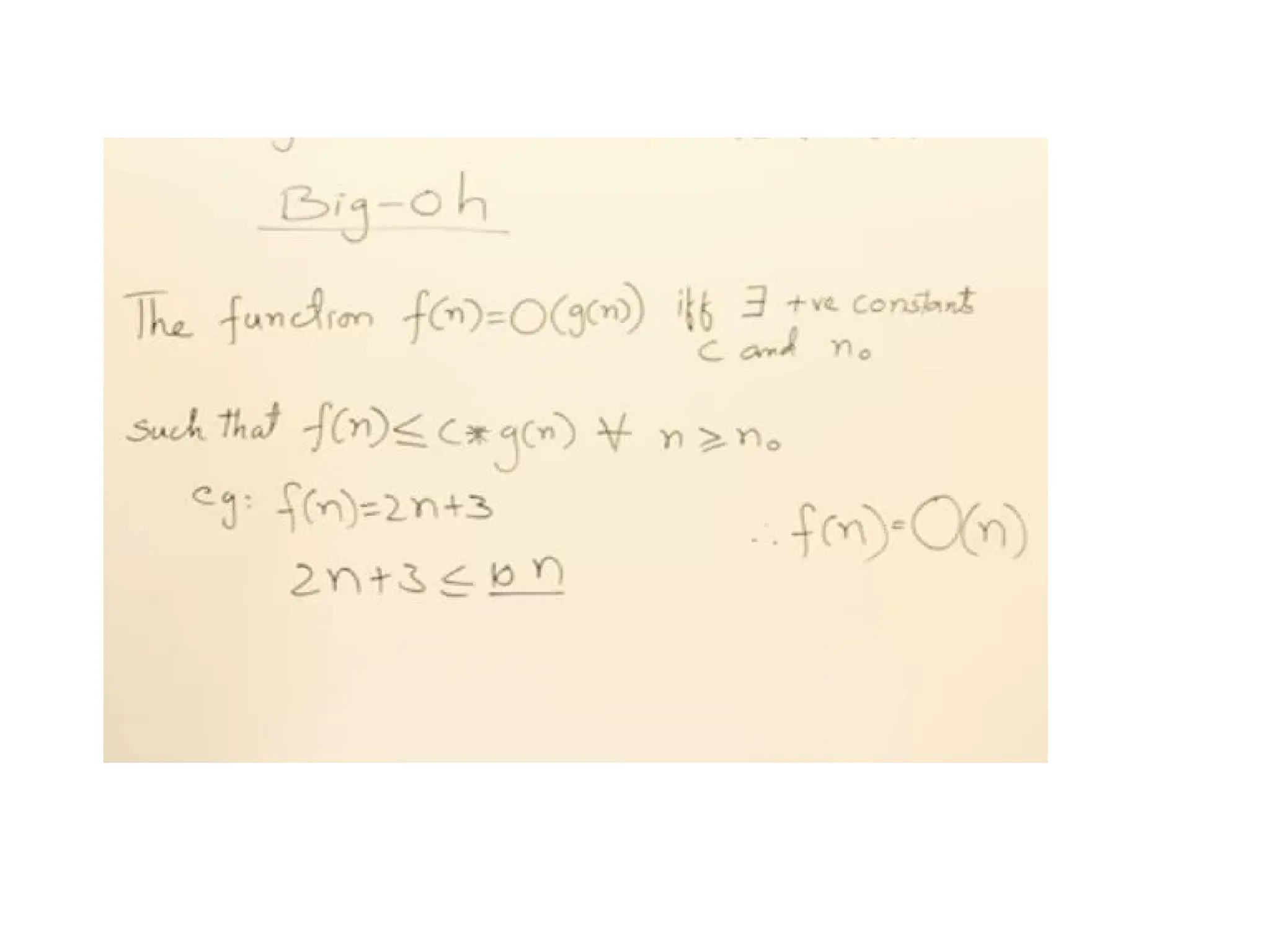
f(n)= O(g(n)) meansthat
– there is a constant c>0, and
– a value n0
such that
f(n)<=c * g(n) for all n>n0
The = sign does not mean equality!
It means that f is an element of the set of functions
which are eventually bounded by (different)
constant multiples of g.
84.
Small Oh-o
f(n)= o(g(n))means that
– there is a constant c>0, and
– a value n0
such that
f(n) <c * g(n) for all n>n0
86.
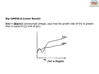
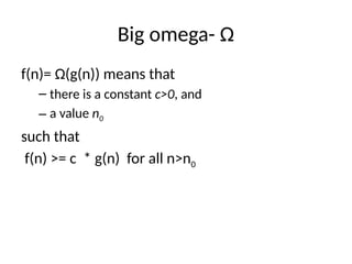
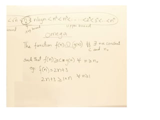
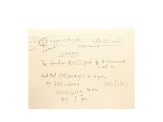
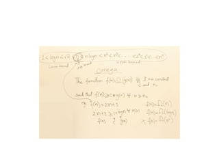
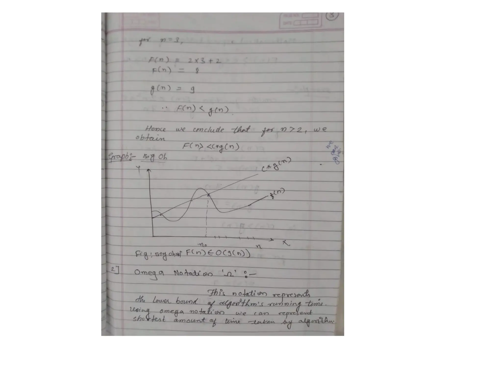
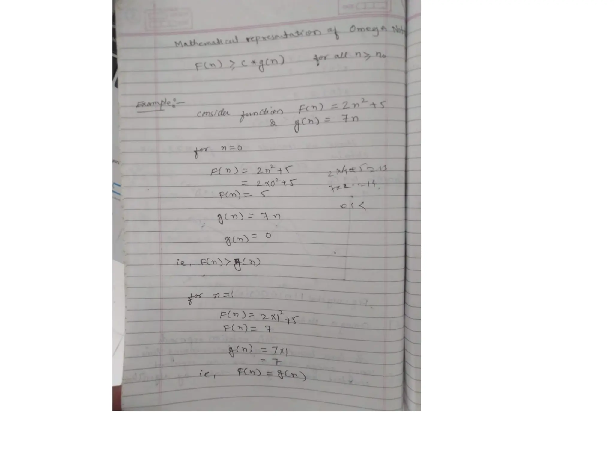
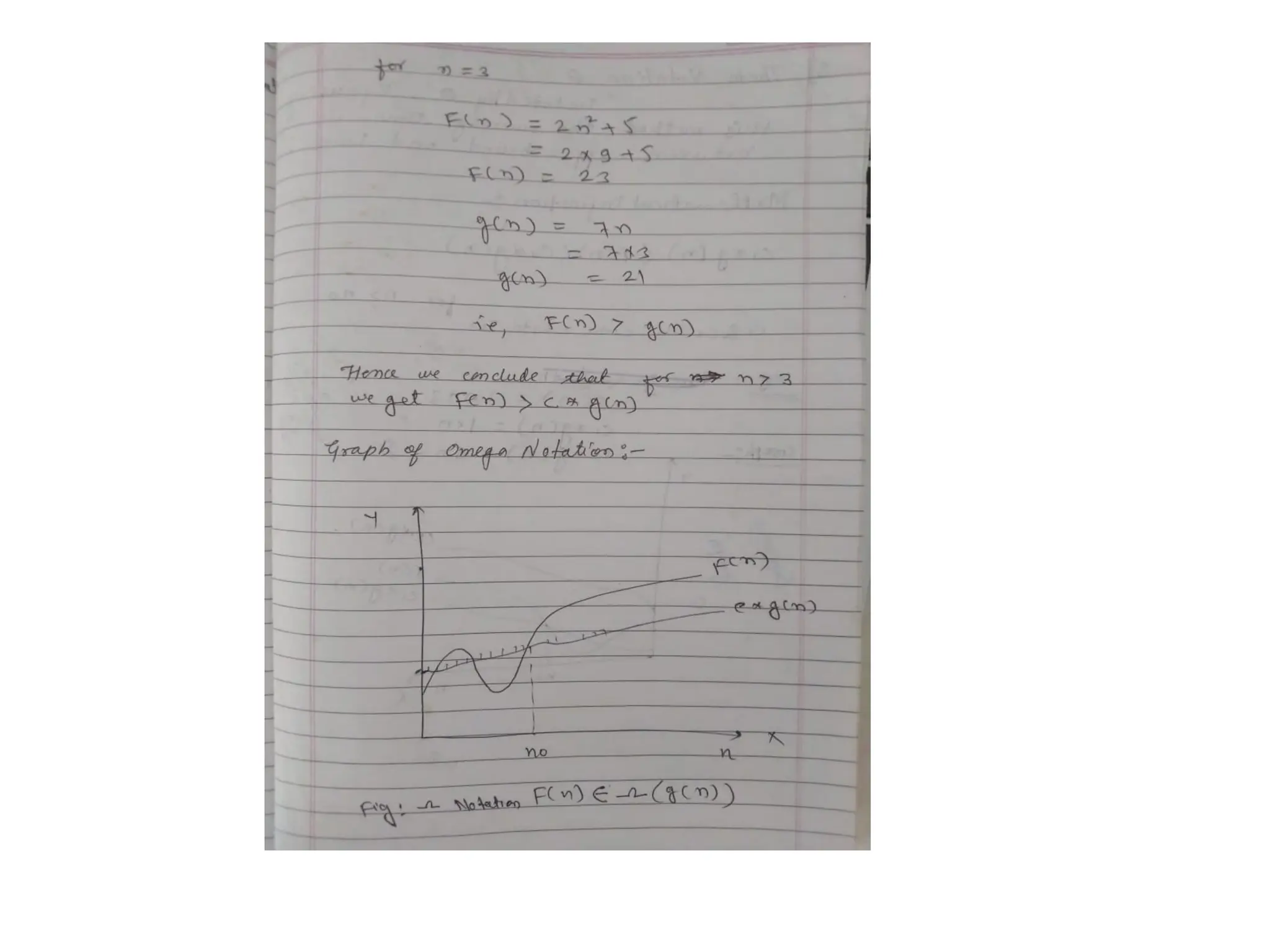
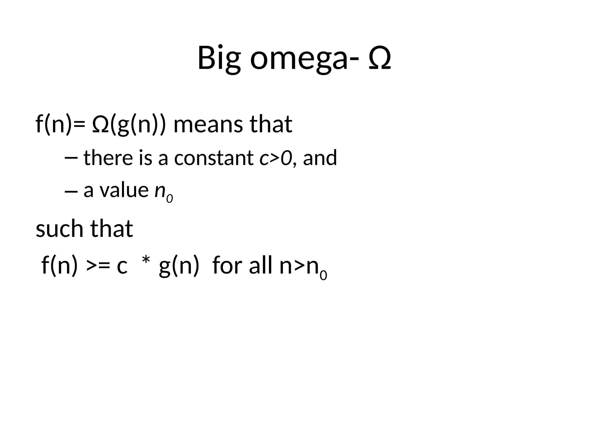
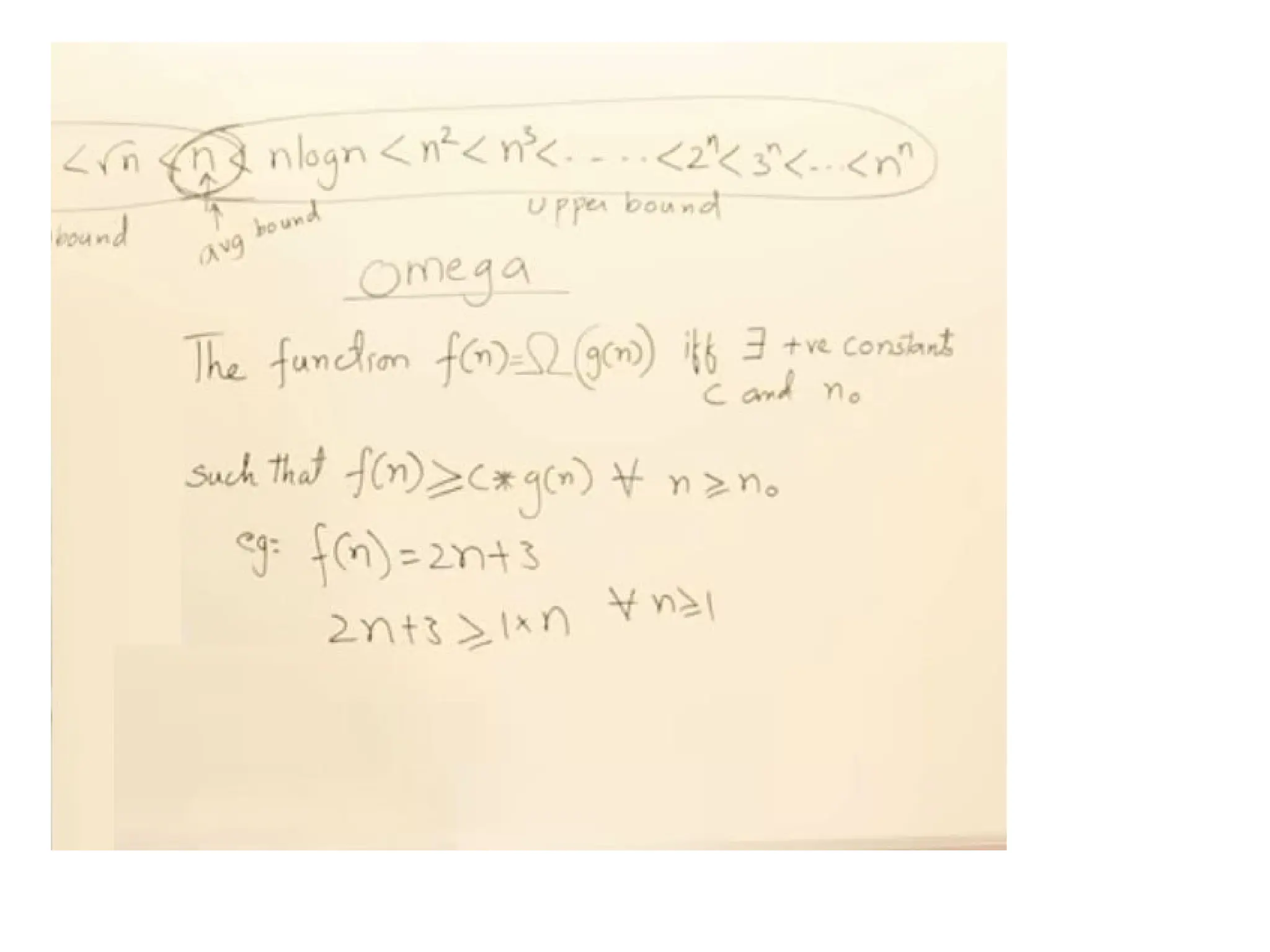
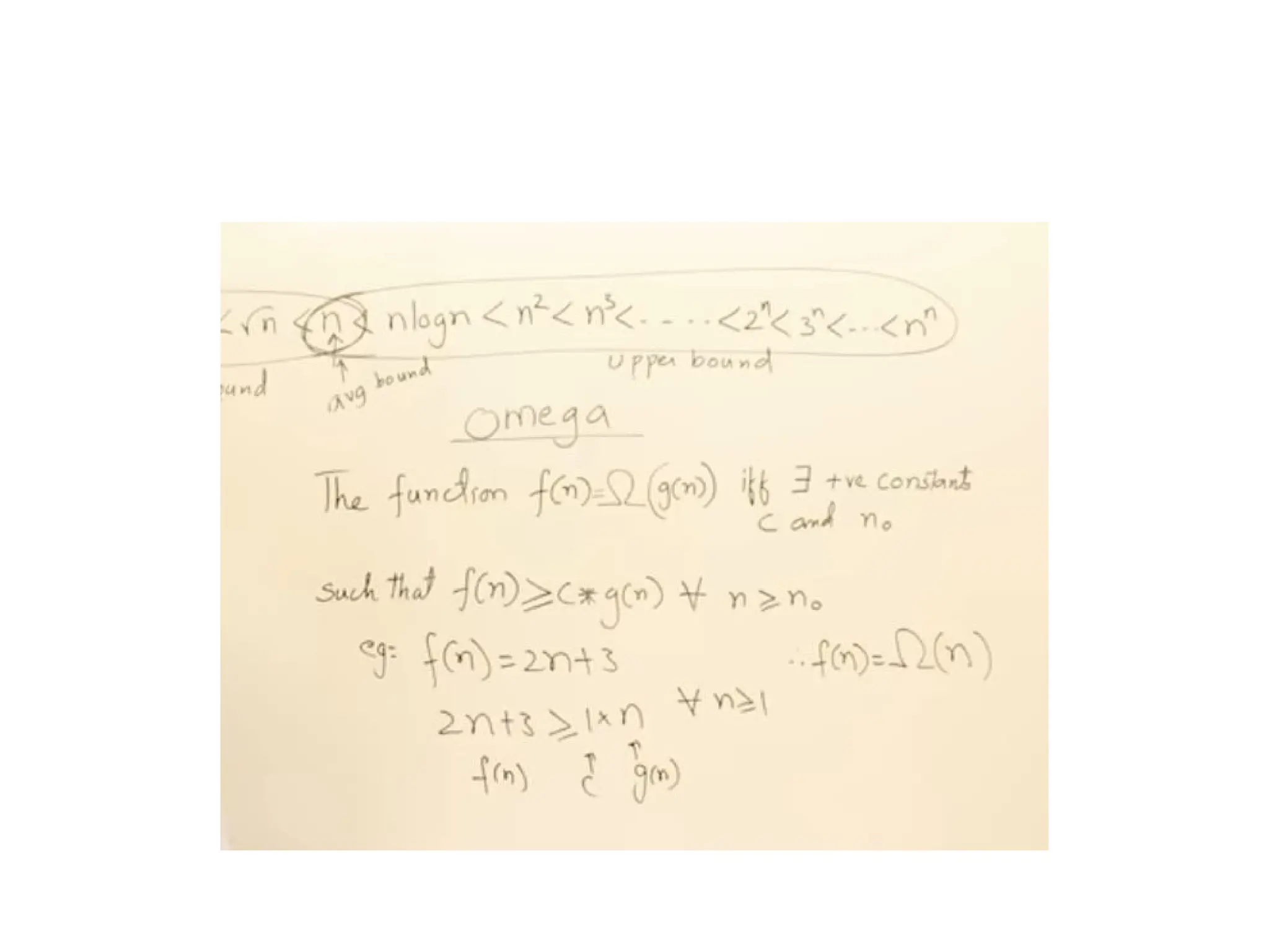
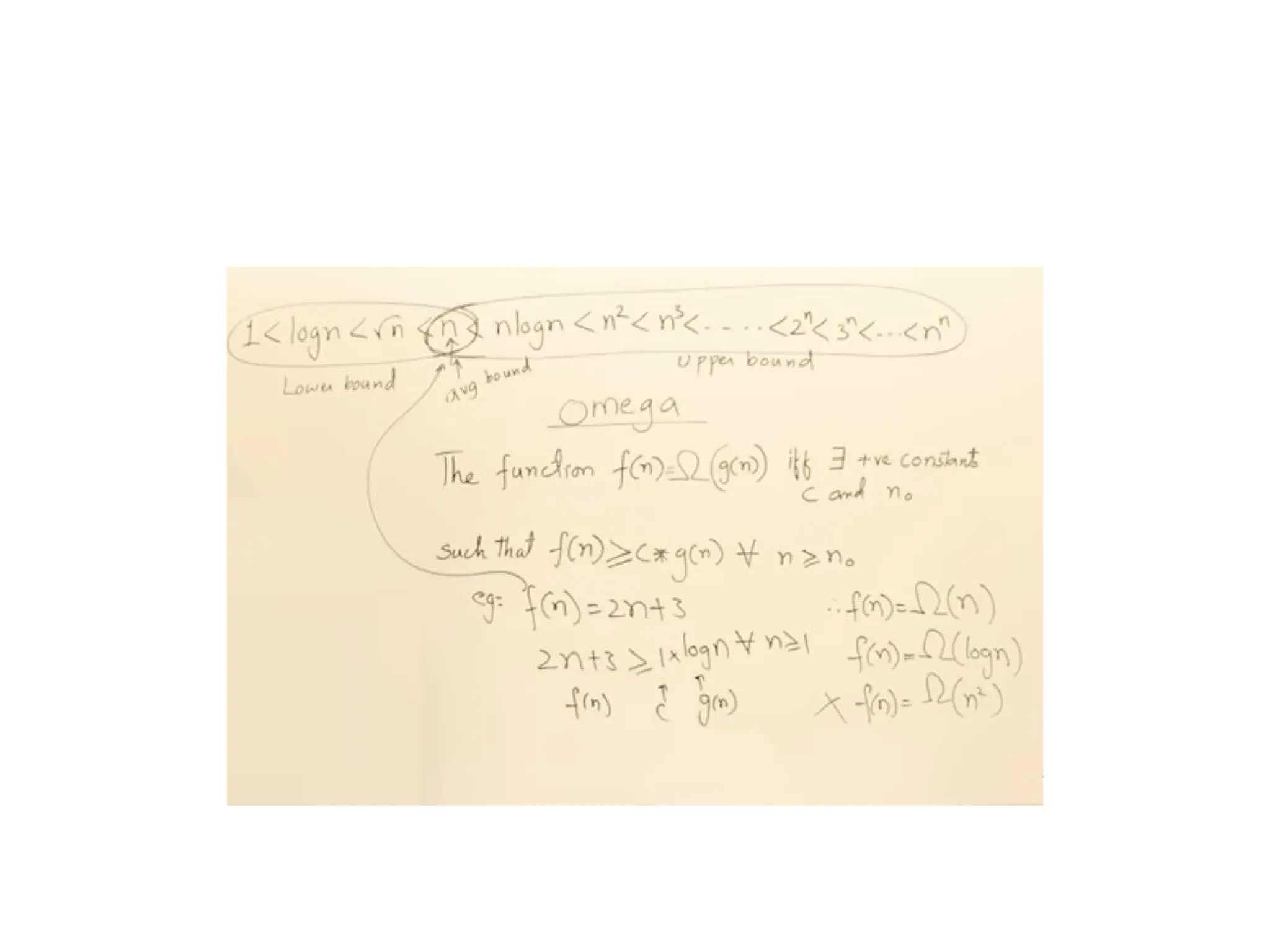
Big omega- Ω
f(n)=Ω(g(n)) means that
– there is a constant c>0, and
– a value n0
such that
f(n) >= c * g(n) for all n>n0
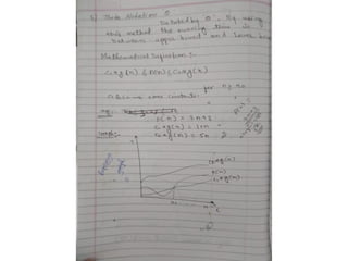
87.
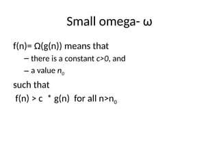
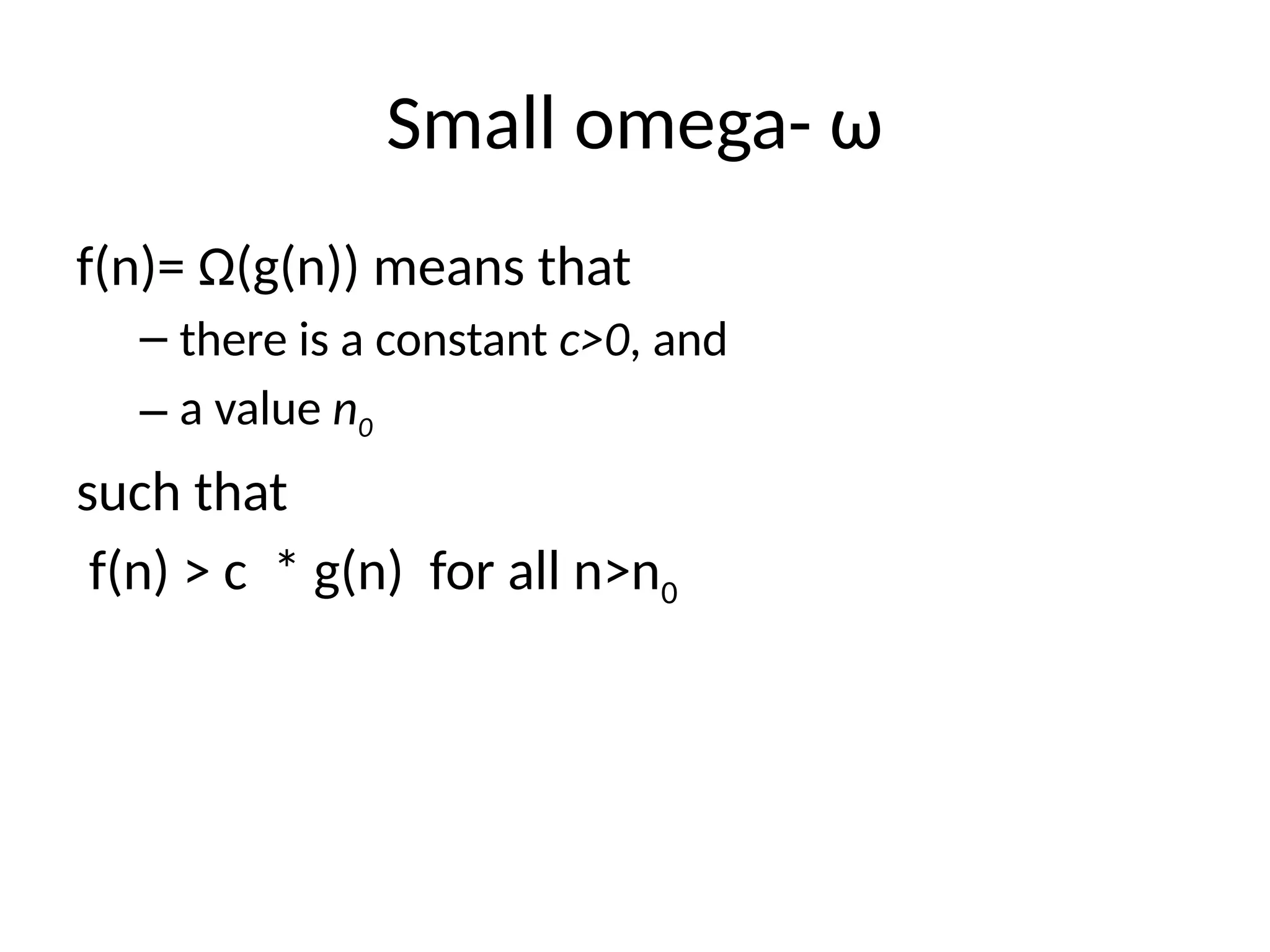
Small omega- ω
f(n)=Ω(g(n)) means that
– there is a constant c>0, and
– a value n0
such that
f(n) > c * g(n) for all n>n0
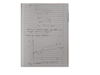
89.
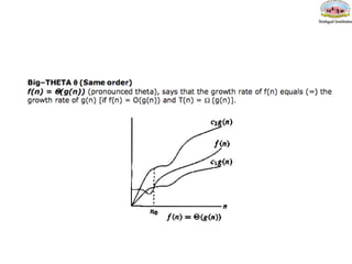
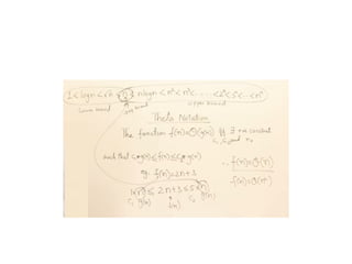
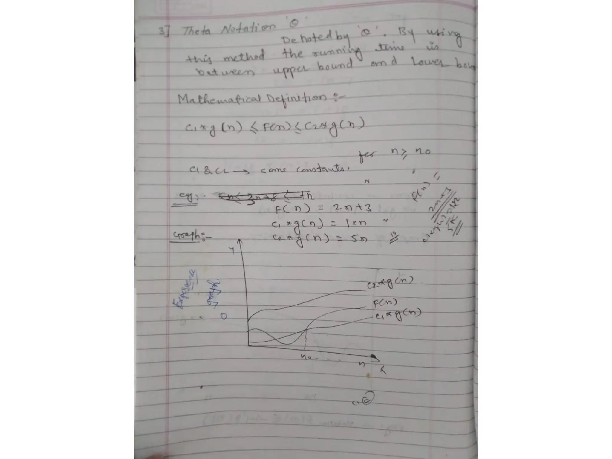
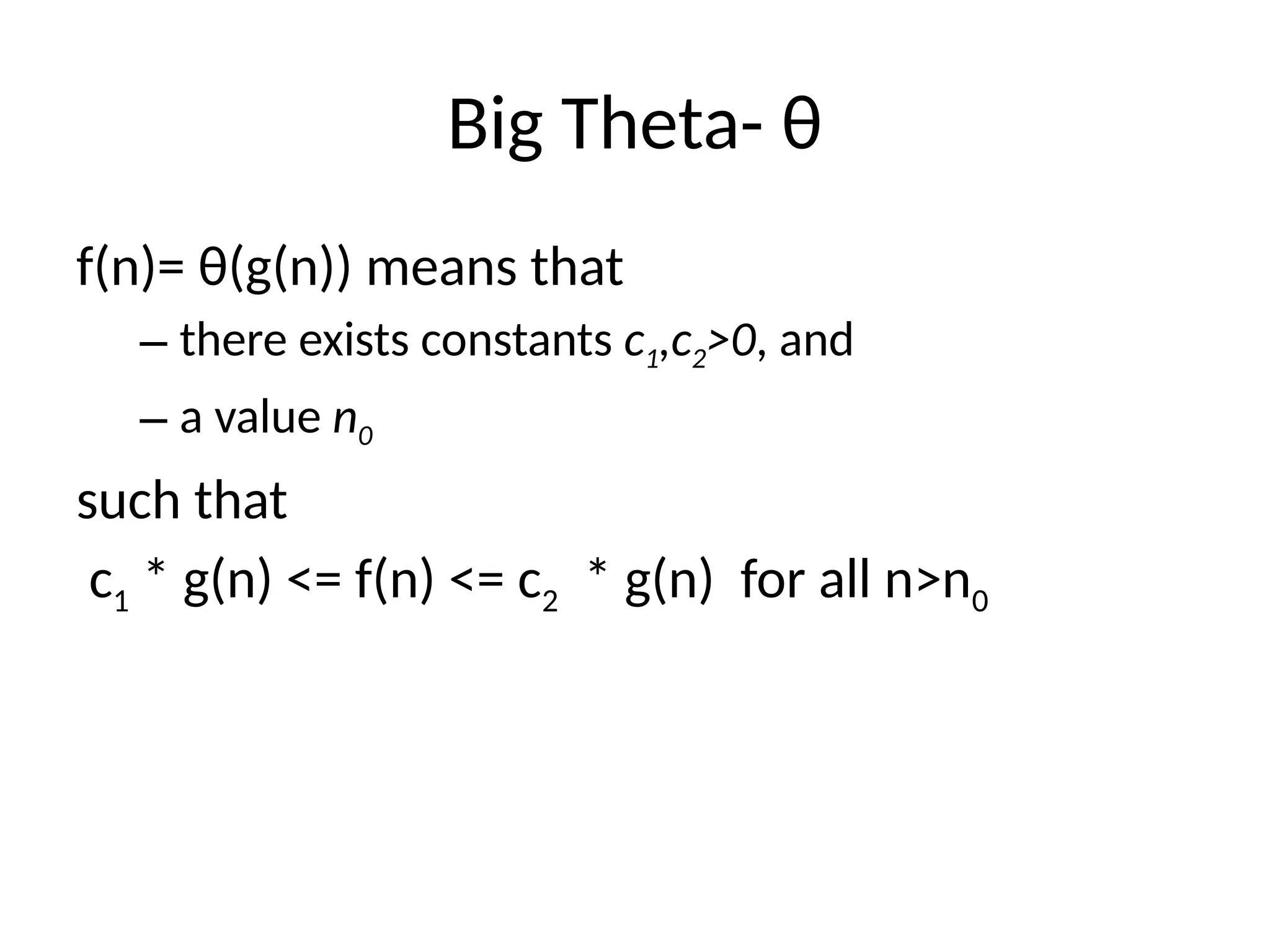
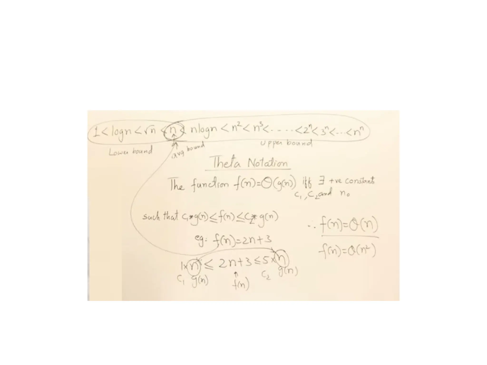
Big Theta- θ
f(n)=θ(g(n)) means that
– there exists constants c1,c2>0, and
– a value n0
such that
c1 * g(n) <= f(n) <= c2 * g(n) for all n>n0
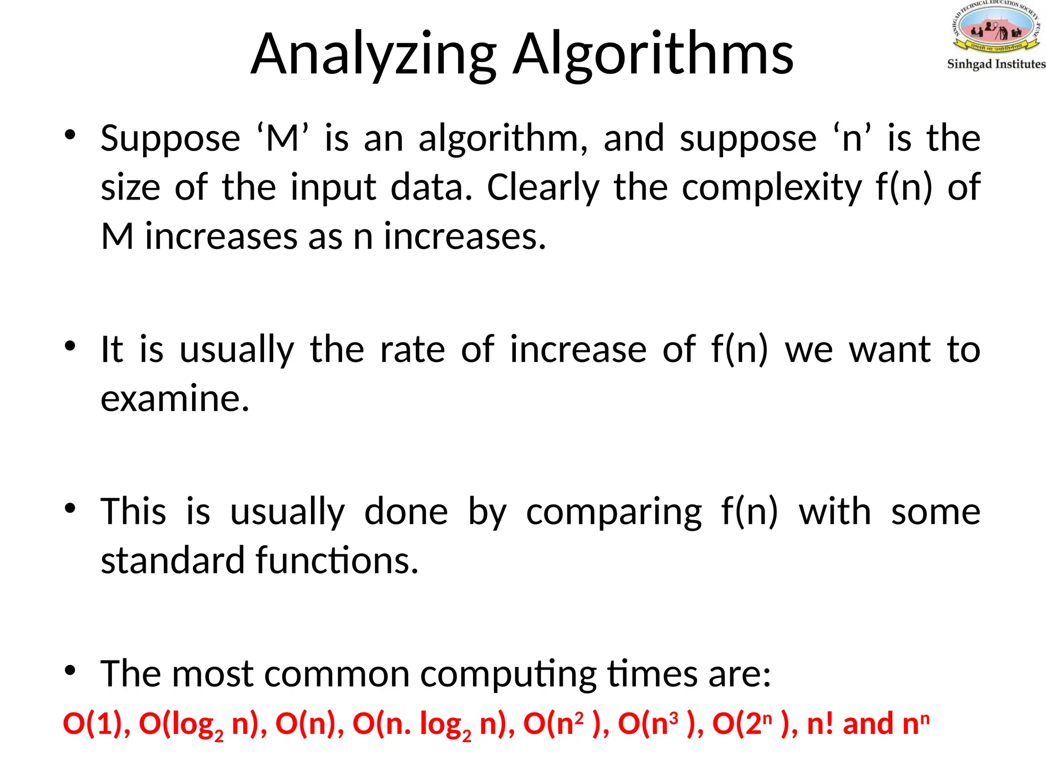
Analyzing Algorithms
• Suppose‘M’ is an algorithm, and suppose ‘n’ is the
size of the input data. Clearly the complexity f(n) of
M increases as n increases.
• It is usually the rate of increase of f(n) we want to
examine.
• This is usually done by comparing f(n) with some
standard functions.
• The most common computing times are:
O(1), O(log2 n), O(n), O(n. log2 n), O(n2
), O(n3
), O(2n
), n! and nn
102.
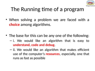
The Running timeof a program
• When solving a problem we are faced with a
choice among algorithms.
• The base for this can be any one of the following:
– i. We would like an algorithm that is easy to
understand, code and debug.
– ii. We would like an algorithm that makes efficient
use of the computer’s resources, especially, one that
runs as fast as possible
103.
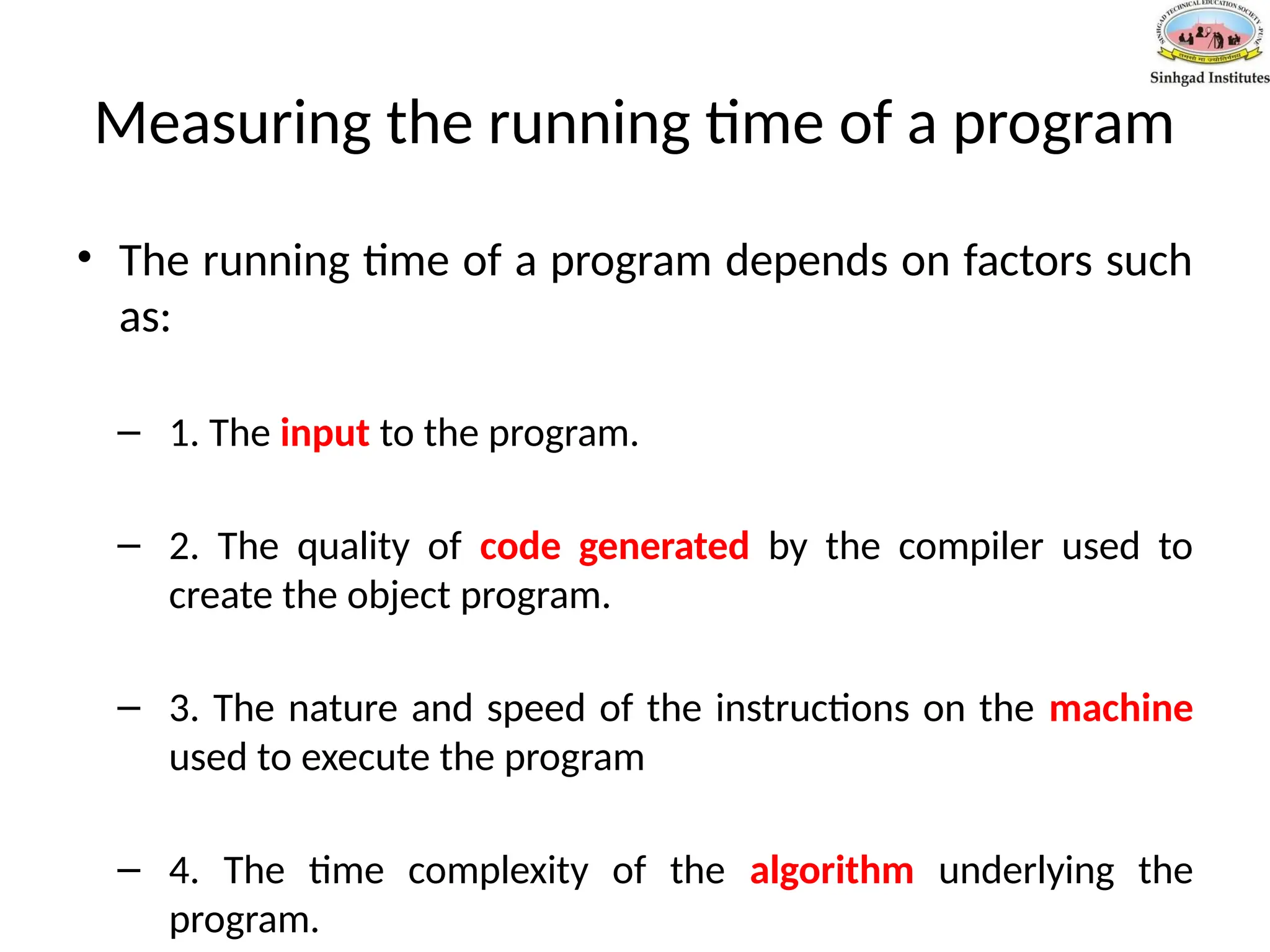
Measuring the runningtime of a program
• The running time of a program depends on factors such
as:
– 1. The input to the program.
– 2. The quality of code generated by the compiler used to
create the object program.
– 3. The nature and speed of the instructions on the machine
used to execute the program
– 4. The time complexity of the algorithm underlying the
program.
110.
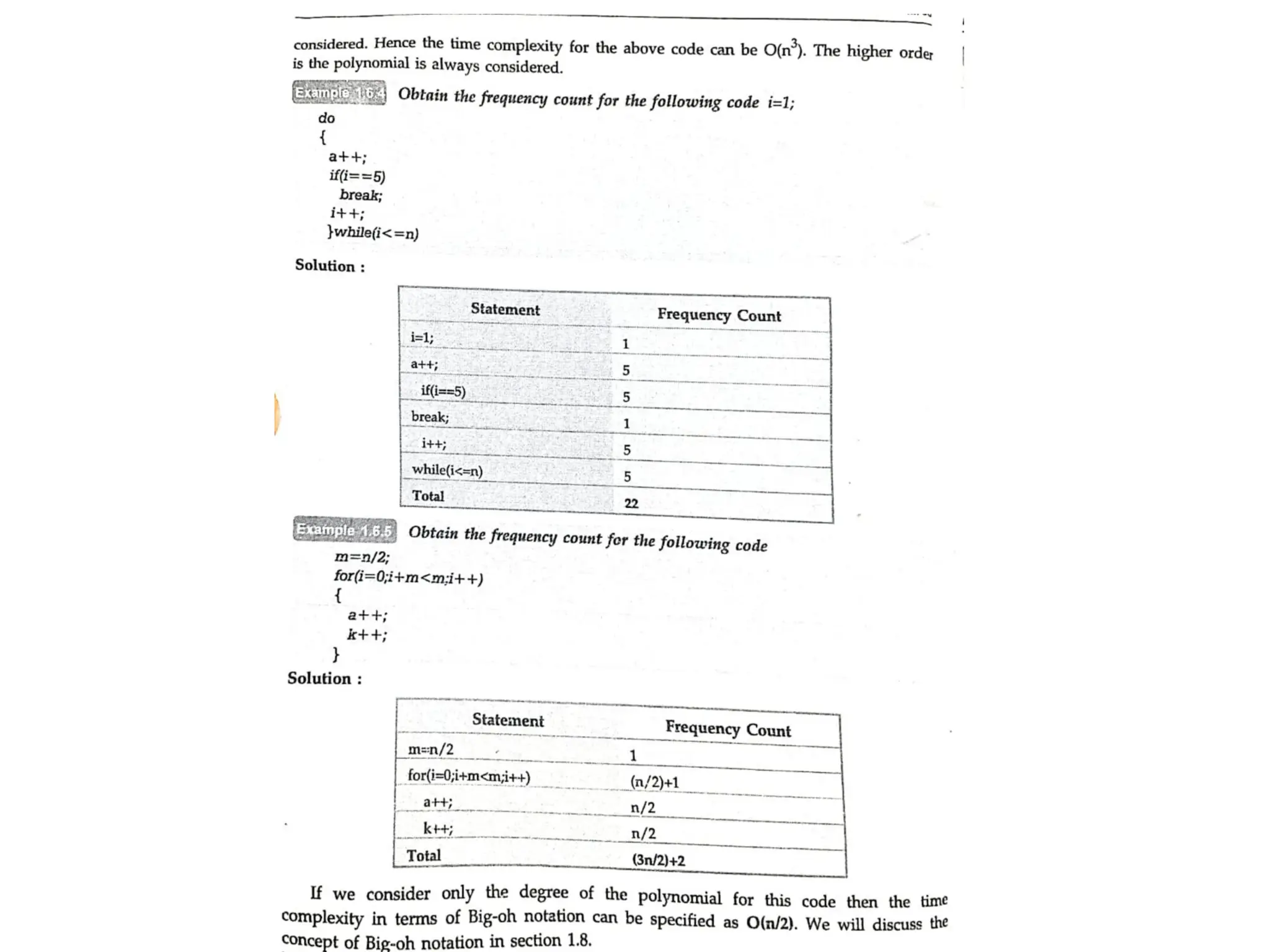
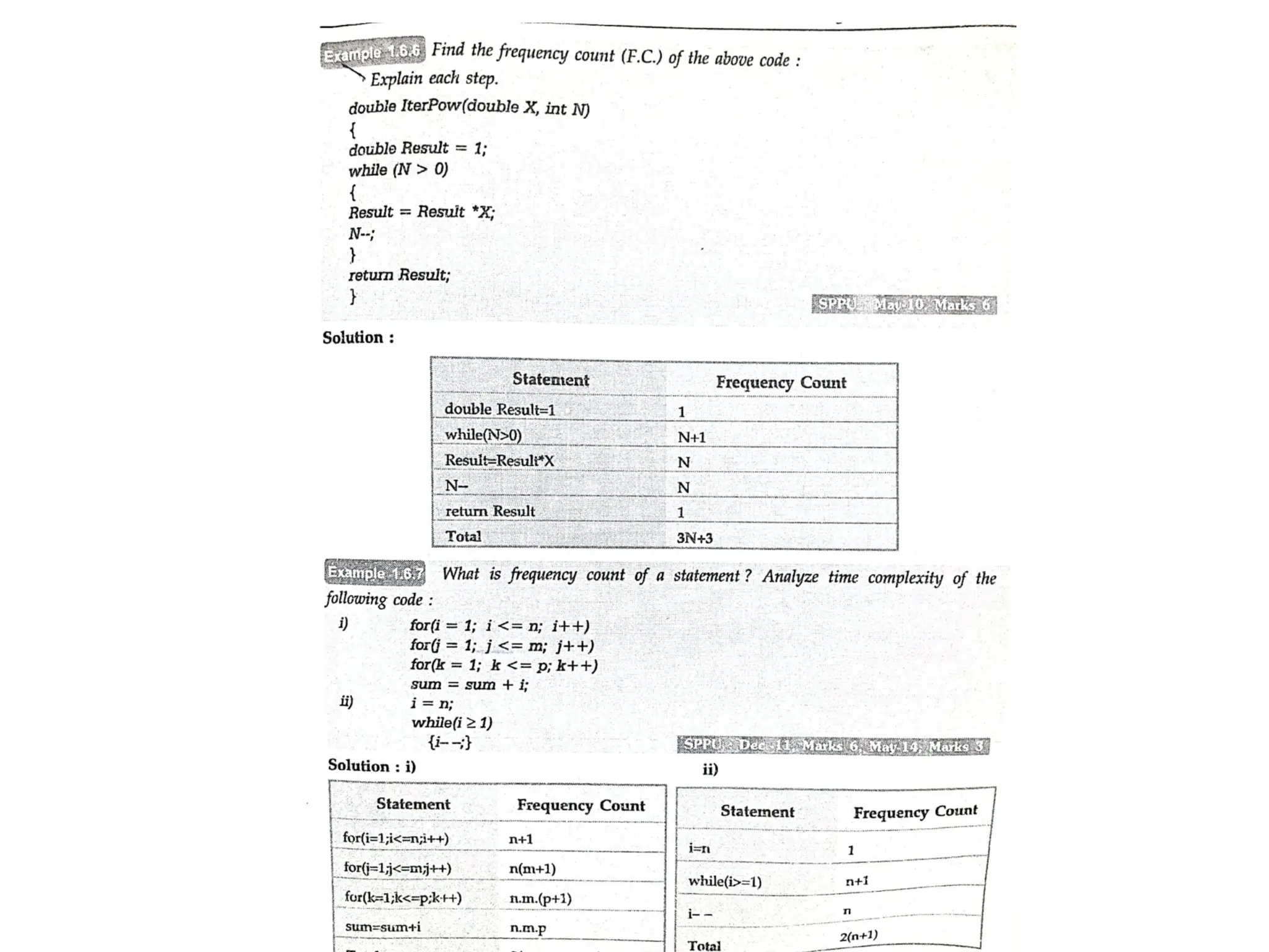
General rules forthe analysis of programs
• In general the running time of a statement or group of
statements may be parameterized by the input size and/or by
one or more variables. The only permissible parameter for the
running time of the whole program is ‘n’ the input size.
1. The running time of each assignment read and write
statement can usually be taken to be O(1). (There are few
exemptions, such as in PL/1, where assignments can involve
arbitrarily larger arrays and in any language that allows function
calls in arraignment statements).
2. The running time of a sequence of statements is determined
by the sum rule. I.e. the running time of the sequence is, to with
in a constant factor, the largest running time of any statement in
the sequence.
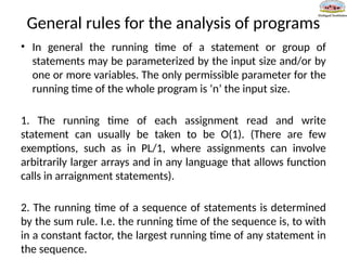
111.
• 3. Therunning time of an if–statement is the cost of
conditionally executed statements, plus the time for
evaluating the condition. The time to evaluate the condition
is normally O(1) the time for an if–then–else construct is
the time to evaluate the condition plus the larger of the
time needed for the statements executed when the
condition is true and the time for the statements executed
when the condition is false.
• 4. The time to execute a loop is the sum, over all times
around the loop, the time to execute the body and the time
to evaluate the condition for termination (usually the latter
is O(1)). Often this time is, neglected constant factors, the
product of the number of times around the loop and the
largest possible time for one execution of the body, but we
must consider each loop separately to make sure.
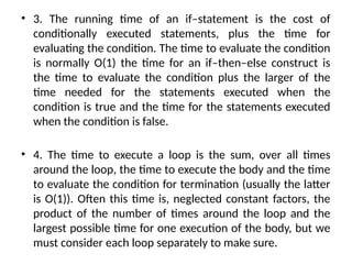
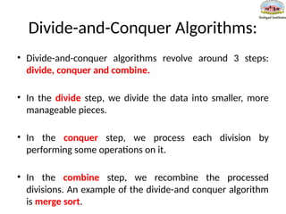
112.
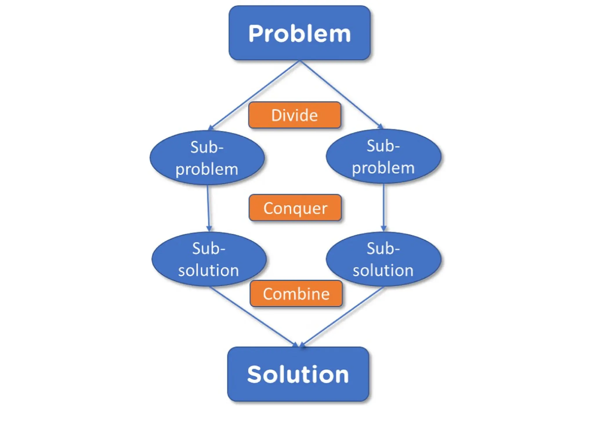
Divide-and-Conquer Algorithms:
• Divide-and-conqueralgorithms revolve around 3 steps:
divide, conquer and combine.
• In the divide step, we divide the data into smaller, more
manageable pieces.
• In the conquer step, we process each division by
performing some operations on it.
• In the combine step, we recombine the processed
divisions. An example of the divide-and conquer algorithm
is merge sort.
115.
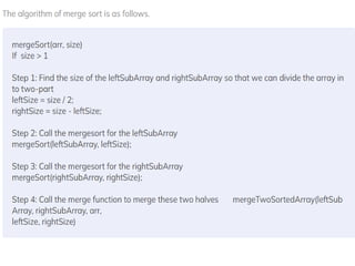
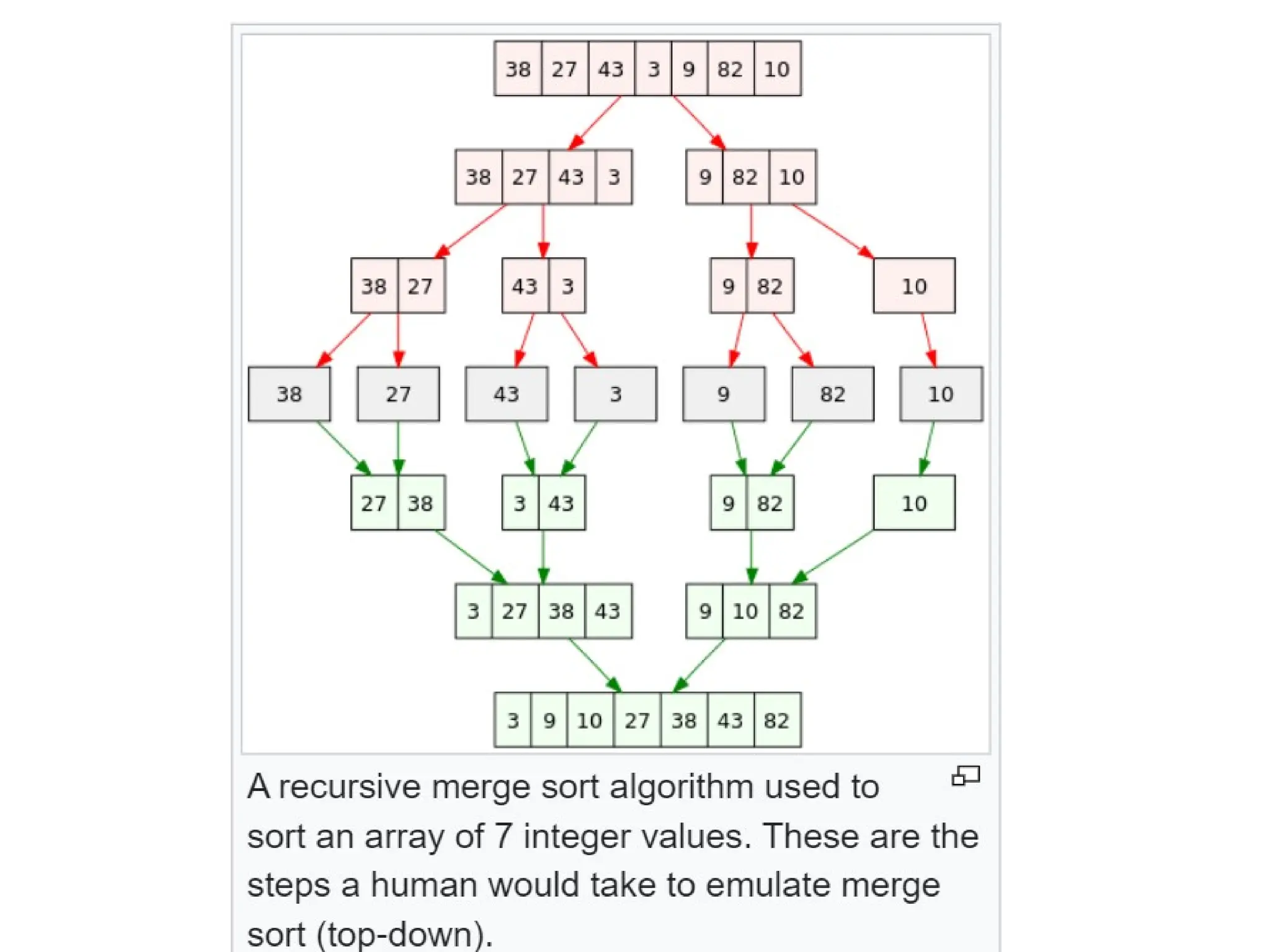
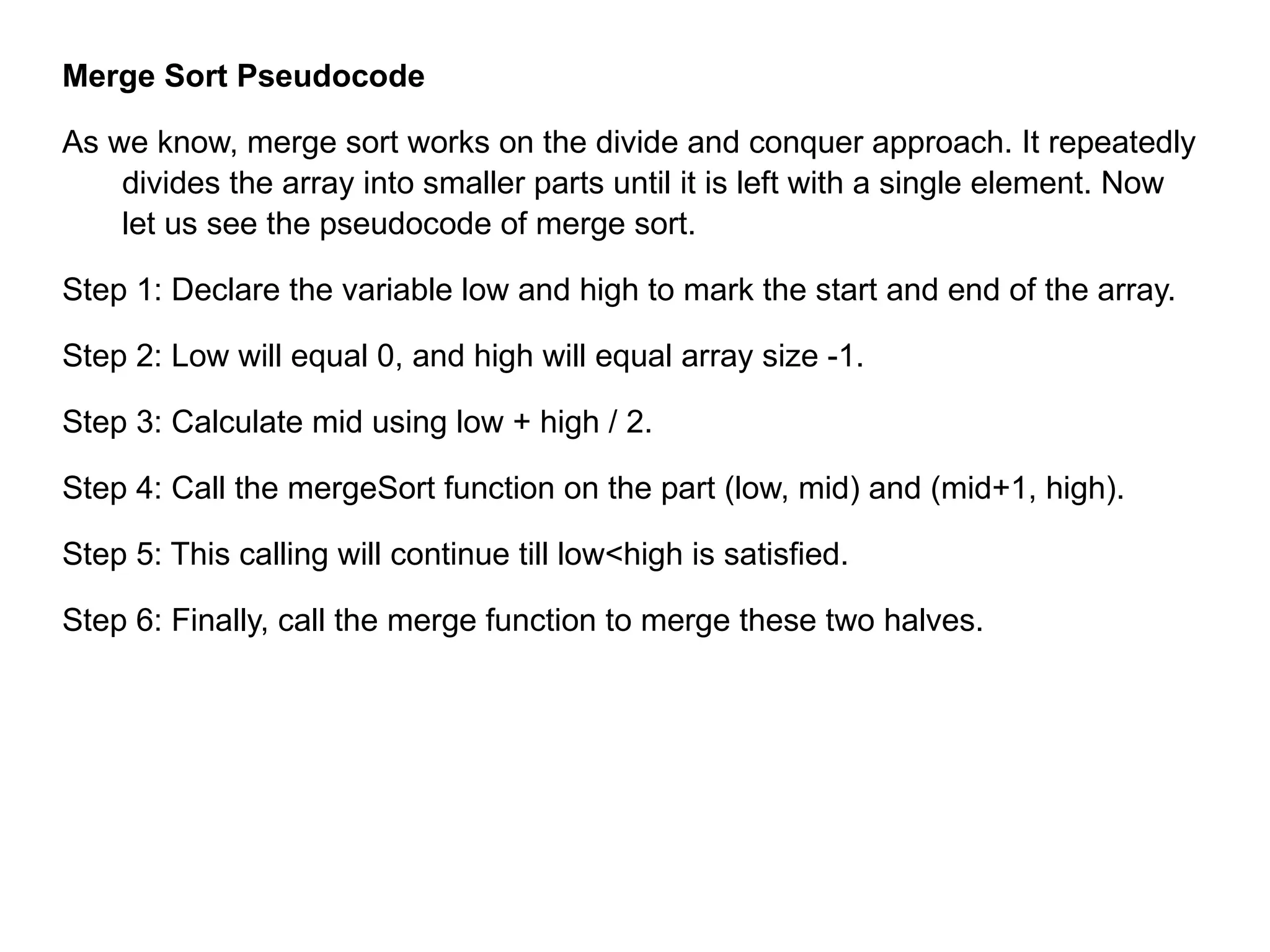
Merge Sort Pseudocode
Aswe know, merge sort works on the divide and conquer approach. It repeatedly
divides the array into smaller parts until it is left with a single element. Now
let us see the pseudocode of merge sort.
Step 1: Declare the variable low and high to mark the start and end of the array.
Step 2: Low will equal 0, and high will equal array size -1.
Step 3: Calculate mid using low + high / 2.
Step 4: Call the mergeSort function on the part (low, mid) and (mid+1, high).
Step 5: This calling will continue till low<high is satisfied.
Step 6: Finally, call the merge function to merge these two halves.
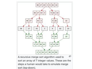
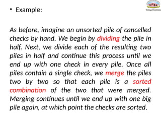
117.
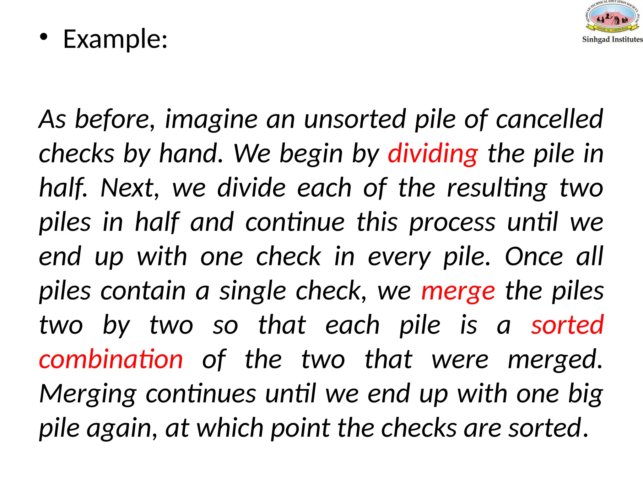
• Example:
As before,imagine an unsorted pile of cancelled
checks by hand. We begin by dividing the pile in
half. Next, we divide each of the resulting two
piles in half and continue this process until we
end up with one check in every pile. Once all
piles contain a single check, we merge the piles
two by two so that each pile is a sorted
combination of the two that were merged.
Merging continues until we end up with one big
pile again, at which point the checks are sorted.
119.
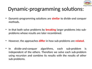
Dynamic-programming solutions:
• Dynamic-programmingsolutions are similar to divide-and conquer
methods.
• In that both solve problems by breaking larger problems into sub-
problems whose results are later recombined.
• However, the approaches differ in how sub-problems are related.
• In divide-and-conquer algorithms, each sub-problem is
independent of the others. Therefore we solve each sub-problem
using recursion and combine its results with the results of other
sub-problems.
120.
• In dynamicprogramming solutions, sub-problems are not
independent of one another.
• A dynamic-programming solution is better than a divide-and
conquer approach because the latter approach will do more
work than necessary, as shared sub-problems are solved more
than once.
• However, if the sub-problems are independent and there is no
repetition, using divide-and-conquer algorithms is much better
than using dynamic-programming.
• Example
Finding the shortest path to reach a point from a vertex in a
weighted graph.
121.
Greedy Algorithms:
• Greedyalgorithms make decisions that look best at the moment.
• In other words, they make decisions that are locally optimal in the hope that
they will lead to globally optimal solutions.
• The greedy method extends the solution with the best possible decision at an
algorithmic stage based on the current local optimum and the best decision
made in a previous stage.
• It is not exhaustive, and does not give accurate answer to many problems. But
when it works, it will be the fastest method.
• Example :
•Huffman coding, which is an algorithm for data compression.
•Prim’s & Kruskal’s Algorithm,
122.
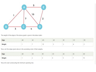
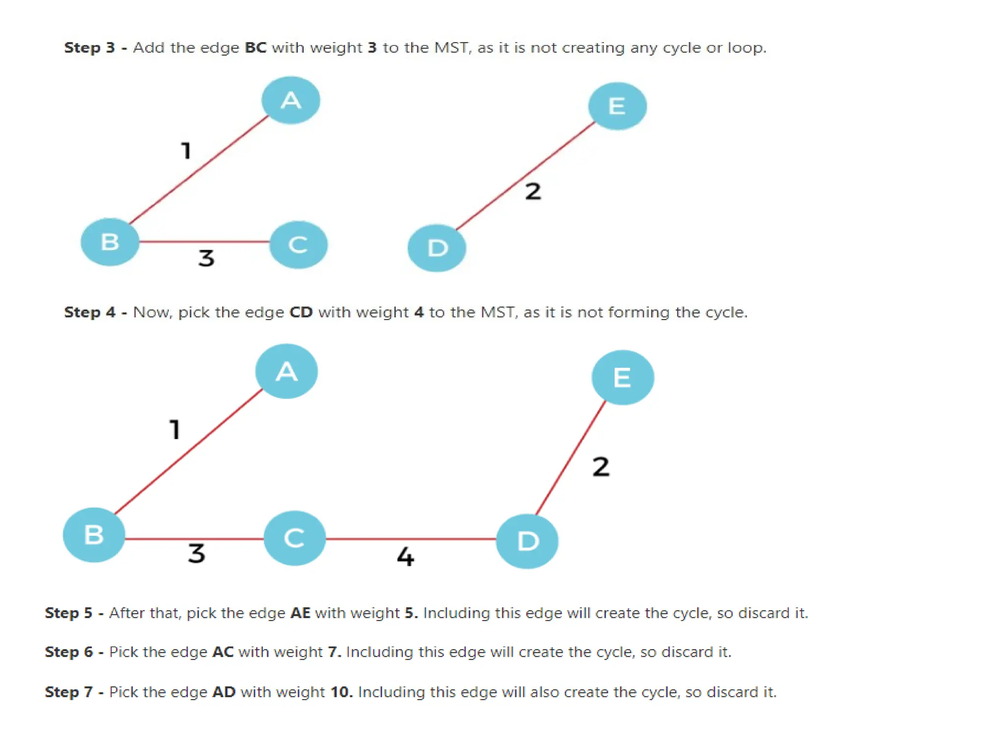
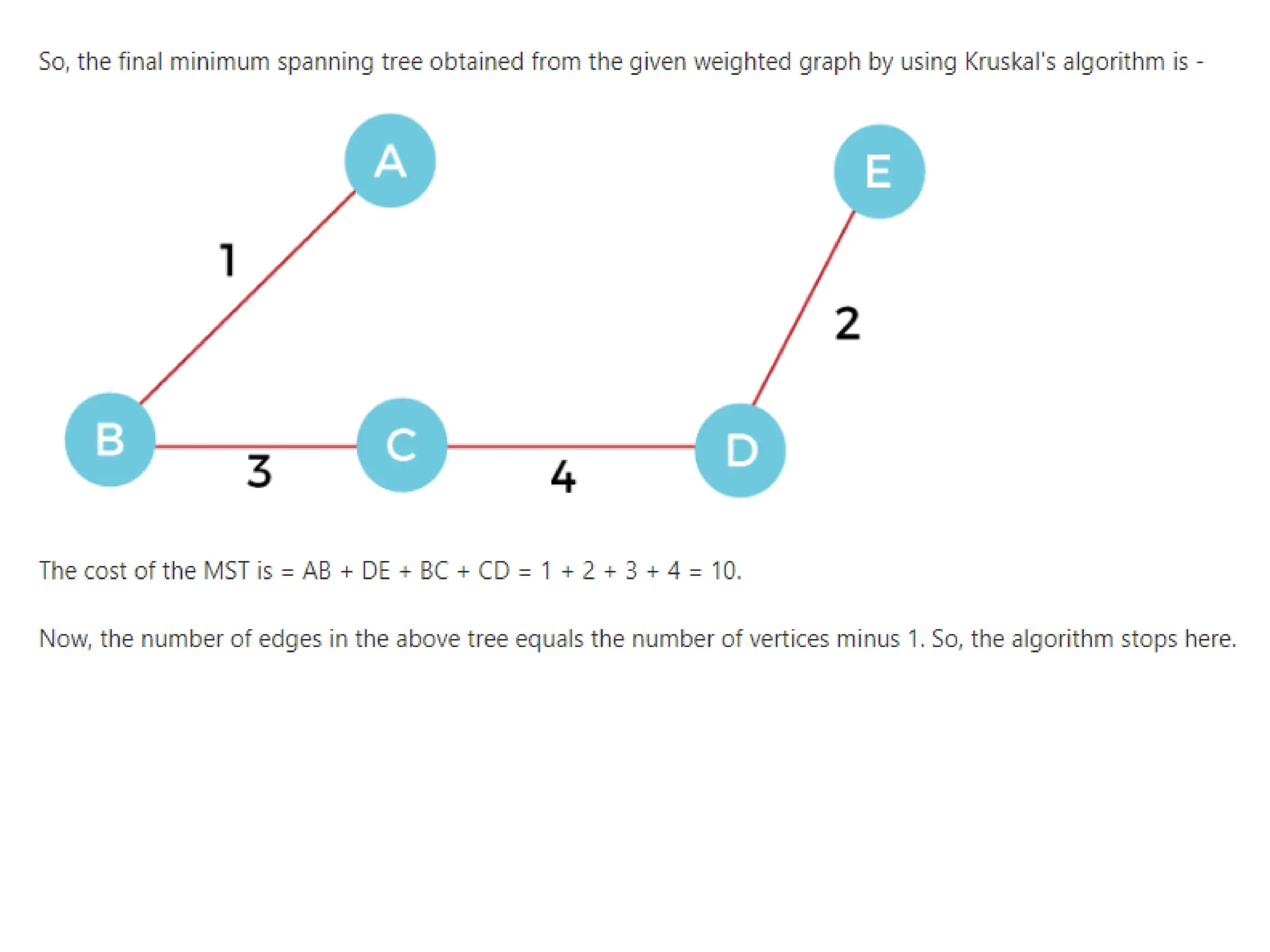
Introduction to Kruskal’sAlgorithm:
Kruskal’s algorithm is used to find the
Minimum Spanning tree (MST) of a given
weighted graph.
How to find MST using Kruskal’s algorithm?
Below are the steps for finding MST using Kruskal’s algorithm:
1. Sort all the edges in non-decreasing order of their weight.
2. Pick the smallest edge. Check if it forms a cycle with the
spanning tree formed so far. If the cycle is not formed, include
this edge. Else, discard it.
3. Repeat step2 until there are (V-1) edges in the spanning
tree.
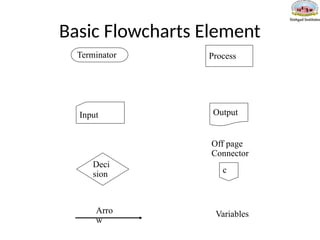
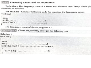
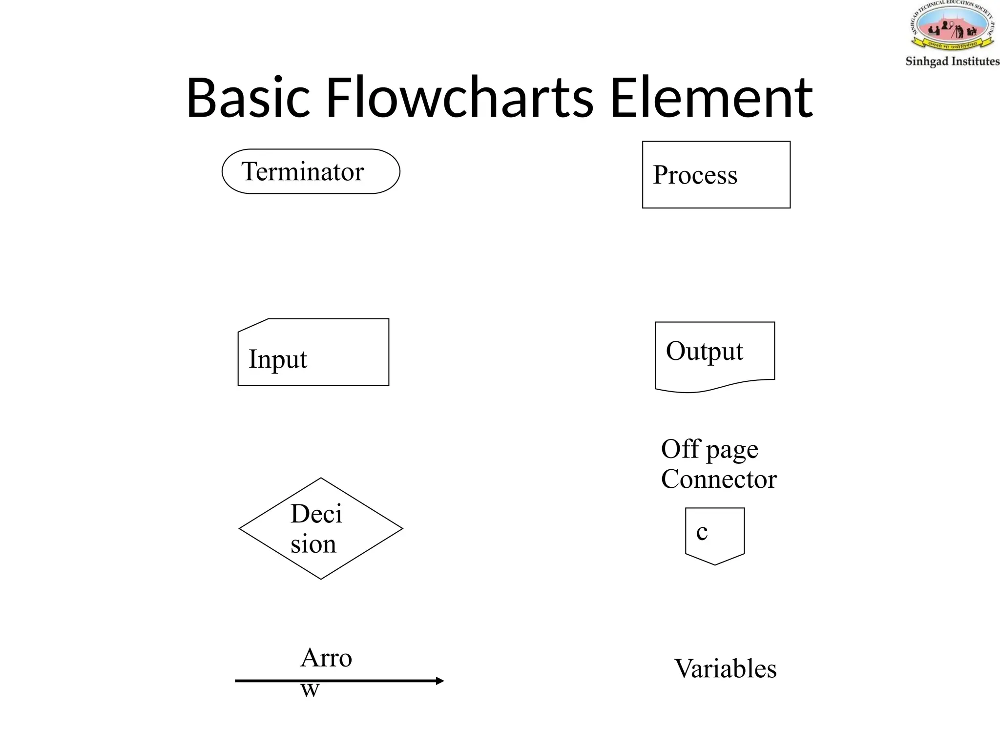
Editor's Notes
#51 Terminator – start or end of algorithm
Process – an atomic activity
Input – get information
Output –display information
Decision – choose between alternatives
Off page connector – use to connect the different parts of a flowchart if it spans multiple pages
Arrow – indicates the order of the steps in an algorithm
Variables – used to store information


![Data Types:
A data type is a term which refers to the kind of data that
variables may hold in a programming language.
Example: int x; [x can hold, integer type data]](https://image.slidesharecdn.com/unit-1introductiontoalgorithmanddatastructures2024-25-251013024710-a62fe9bd/85/Unit-1-Introduction-to-Algorithm-and-Data-Structures-10-320.jpg)


![Data Types:
A data type is a term which refers to the kind of data that
variables may hold in a programming language.
Example: int x; [x can hold, integer type data]](https://image.slidesharecdn.com/unit-1introductiontoalgorithmanddatastructures2024-25-251013024710-a62fe9bd/75/Unit-1-Introduction-to-Algorithm-and-Data-Structures-10-2048.jpg)


![UiPath Automation Suite Installation (Hands-On) [2/3]](https://cdn.slidesharecdn.com/ss_thumbnails/automationsuitecommunitysession2-251015095633-a6d862f1-thumbnail.jpg?width=600ounds&width=560&fit=bounds)

