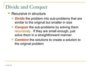
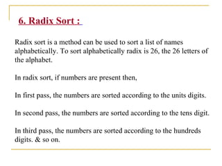
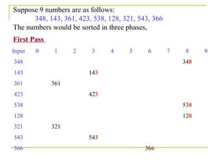
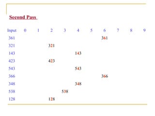
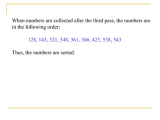
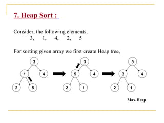
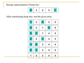
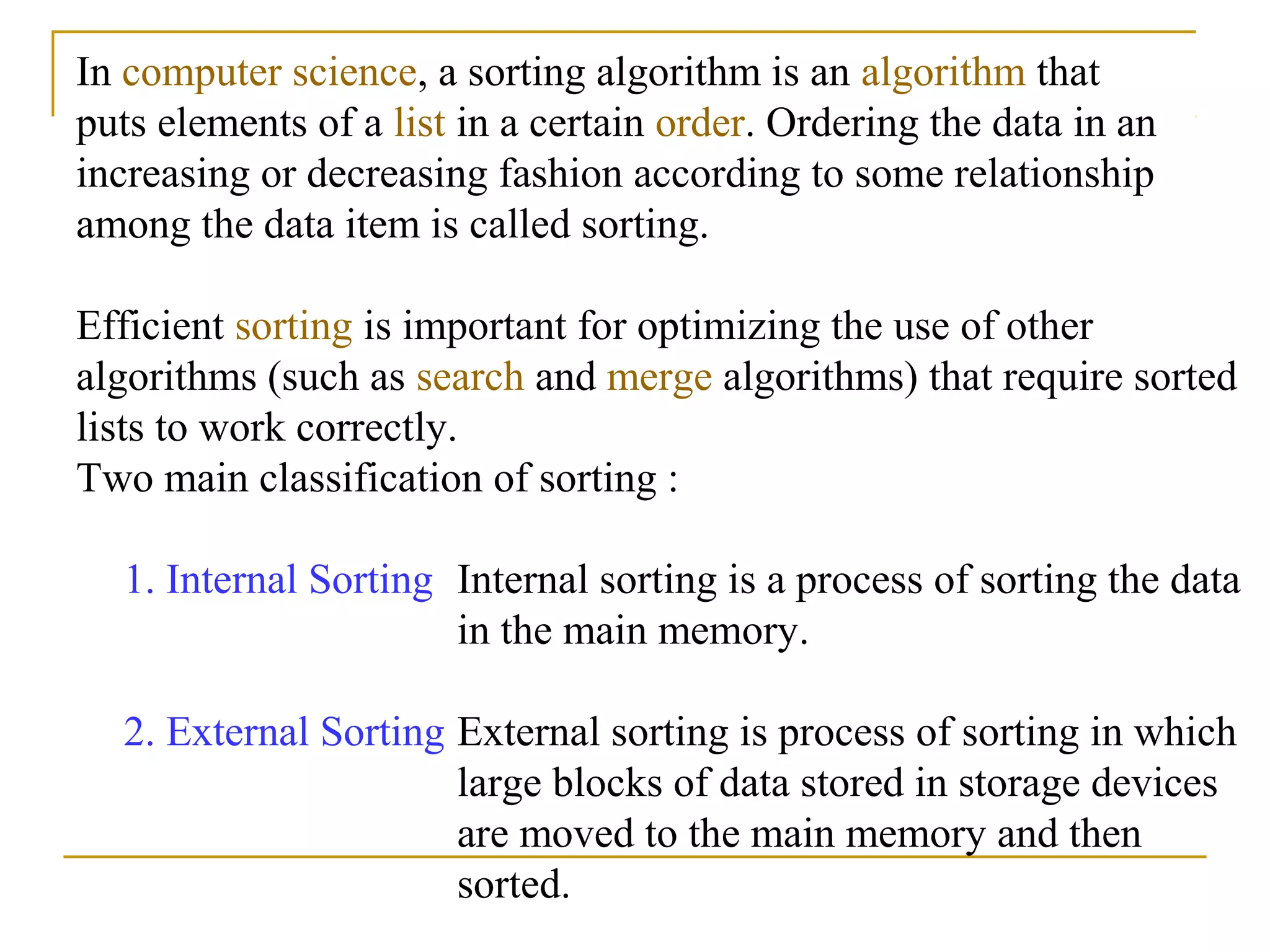
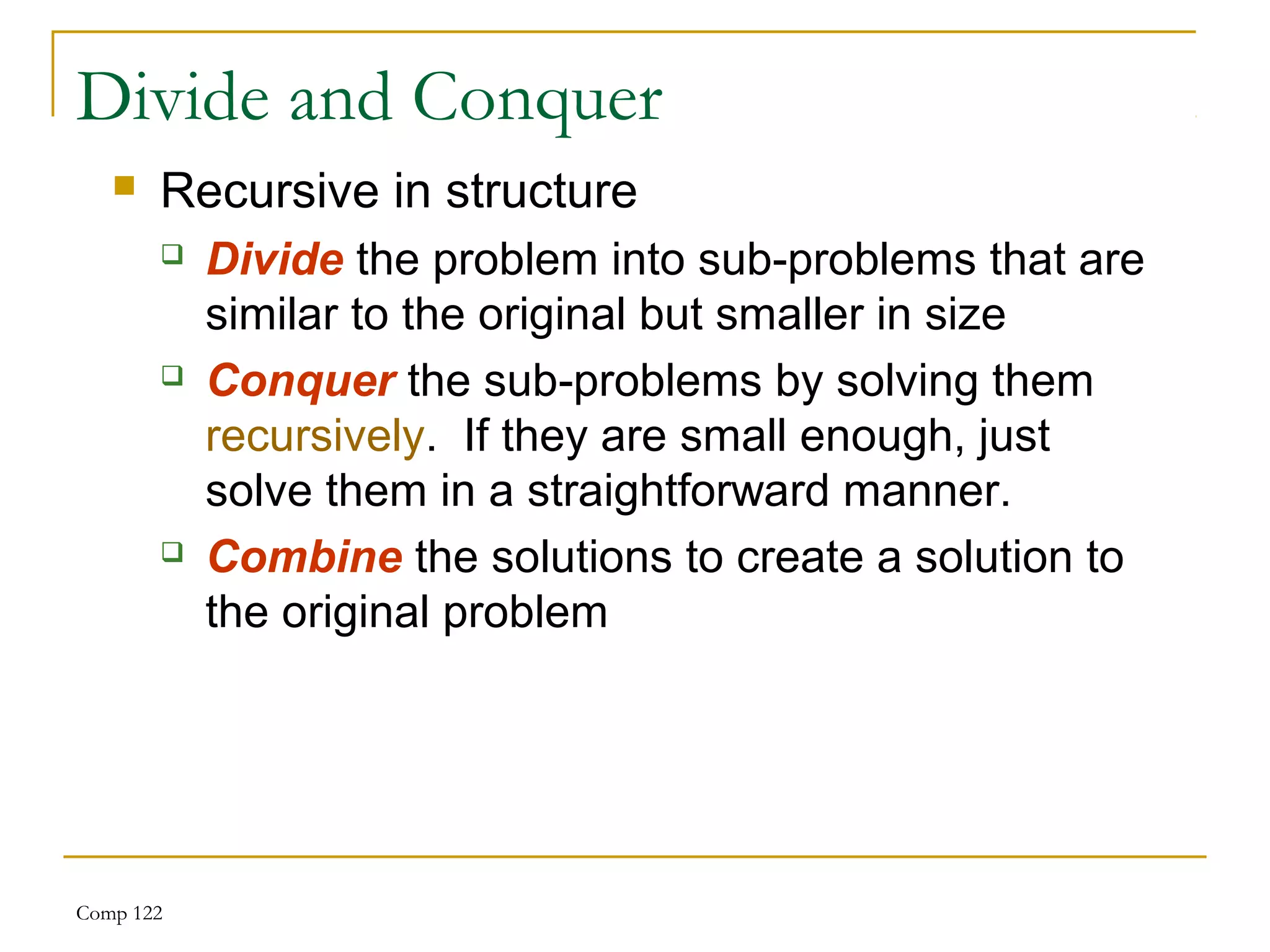
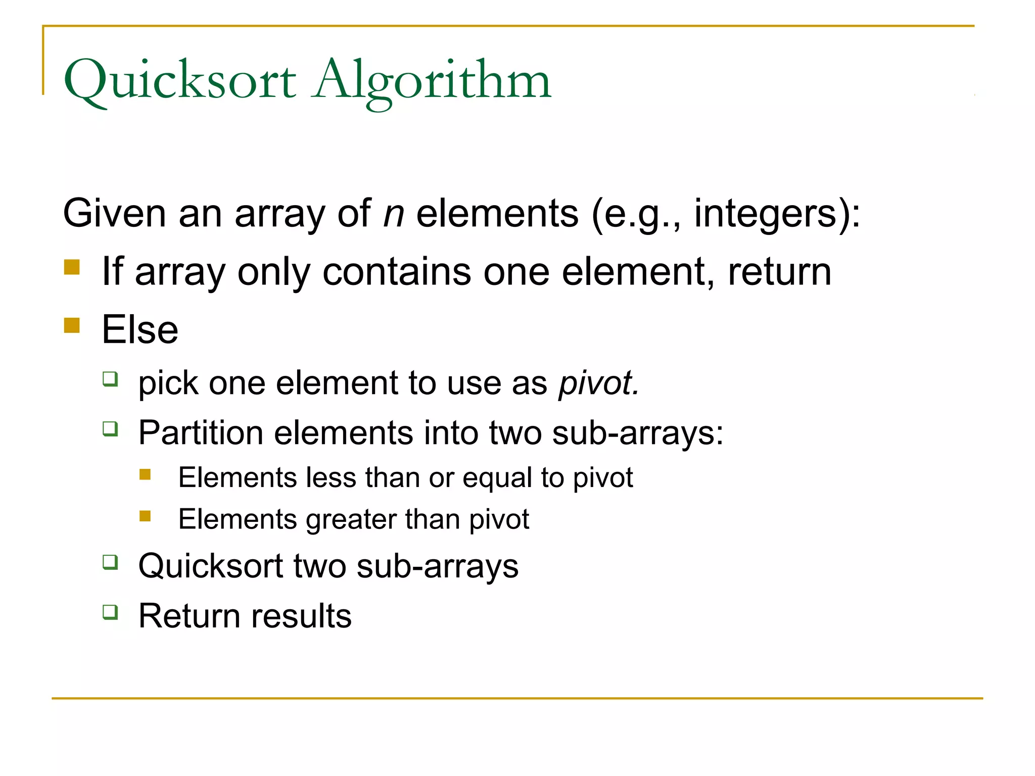
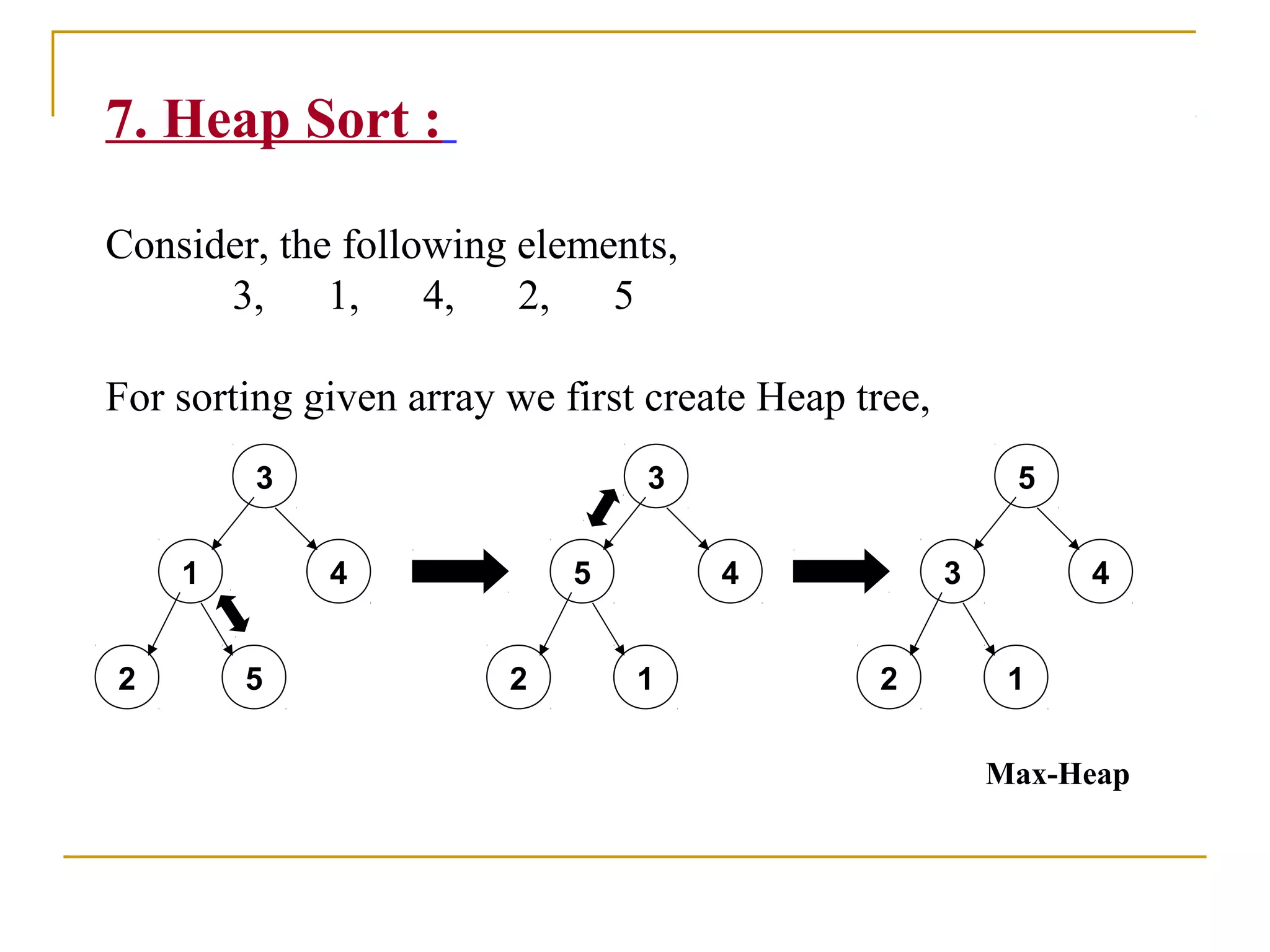
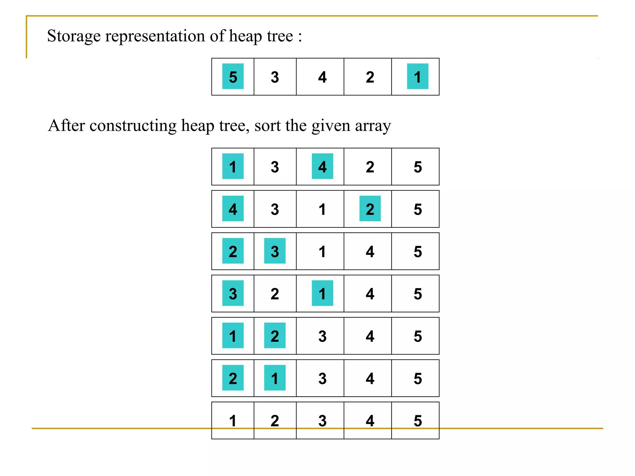
The document discusses various sorting algorithms including insertion sort, selection sort, bubble sort, merge sort, and quick sort. It provides detailed explanations of how each algorithm works through examples using arrays or lists of numbers. The key steps of each algorithm are outlined in pseudocode to demonstrate how they sort a set of data in either ascending or descending order.

![1.Insertion Sort :
Suppose an array A with n elements A[1], A[2],…..,A[n] is in
memory. The insertion sort algorithm. Scans A from A[1] to A[n],
inserting each element A[K] into its proper position in the
previously sorted sub array A[1], A[2], …,A[K-1]. That is:
Pass 1: A[1] by itself is trivially sorted.
Pass 2: A[2] is inserted either before or after A[1] so that A[1], A[2]
is sorted.
Pass 3: A[3] is inserted into its proper place in A[1], A[2], that is
before A[1], between A[1] and A[2], or after A[2], So that
A[1], A[2],A[3] is sorted.](https://image.slidesharecdn.com/unit7-sorting-180714073502/85/Unit-7-sorting-3-320.jpg)
![Pass 4: A[4] is inserted into its proper place in A[1],A[2],A[3]
so that:
A[1],A[2],A[3],A[4] is sorted.
.
.
.
.
.
Pass N : A[N] is inserted into its proper place in
A[1],A[2],…,A[N-1] so that :
A[1],A[2],……,A[N] is sorted.](https://image.slidesharecdn.com/unit7-sorting-180714073502/85/Unit-7-sorting-4-320.jpg)
![Algorithm :
INSERTION(A,N)
1. Set A[0] := -∞ [Initializes element]
2. Repeat Steps 3 to 5 for K = 2,3,…..,N:
3. Set TEMP := A[K] and PTR := K-1
4. Repeat while TEMP < A[PTR]:
1. Set A[PTR + 1] := A[PTR]. [Moves element
forward.]
2. Set PTR := PTR – 1
5. Set A[PTR + 1] := TEMP [Inserts element in proper
place.]
[End of Step 2 loop.]
6. Return](https://image.slidesharecdn.com/unit7-sorting-180714073502/85/Unit-7-sorting-5-320.jpg)
![Pass A[0] A[1] A[2] A[3] A[4] A[5] A[6] A[7] A[8]
K=1: -∞ 33 44 11 88 22 66 55
K=2: -∞ 77 33 44 11 88 22 66 55
K=3: -∞ 33 77 44 11 88 22 66 55
K=4: -∞ 33 44 77 11 88 22 66 55
K=5: -∞ 11 33 44 77 88 22 66 55
K=6: -∞ 11 33 44 77 88 22 66 55
K=7: -∞ 11 22 33 44 77 88 66 55
K=8: -∞ 11 22 33 44 66 77 88 55
Sorted: -∞ 11 22 33 44 55 66 77 88
Array A is, 77, 33, 44, 11, 88, 22, 66, 55
77](https://image.slidesharecdn.com/unit7-sorting-180714073502/85/Unit-7-sorting-6-320.jpg)
![2. Selection Sort :
Suppose an array A with n elements A[1], A[2],…..,A[n] is in
memory. The selection sort algo. For sorting A as follows:
Pass 1: Find the location LOC of the smallest in the list of N elements
A[1],A[2],….,A[N], and then interchange A[LOC] and A[1],
Then : A[1] is sorted.
Pass 2: Find the location LOC of the smallest in the sublist of N-1
elements A[1],A[2],….,A[N], and then interchange A[LOC]
and A[2], Then : A[1], A[2]is sorted. Since A[1] <= A[2].
Pass 3:Find the location LOC of the smallest in the sub list of N-2
elements A[1],A[2],….,A[N], and then interchange A[LOC]
and A[3], Then : A[1], A[2],A[3]is sorted. Since A[2] <= A[3].](https://image.slidesharecdn.com/unit7-sorting-180714073502/85/Unit-7-sorting-7-320.jpg)
![.
.
.
Pass N-1:Find the location LOC of the smaller of the elements
A[N-1],A[N], and then interchange A[LOC] and A[N-
1], Then : A[1],A[2],….A[N]is sorted.
Since A[N-1] <= A[N].
Thus A is sorted after N-1 passes.](https://image.slidesharecdn.com/unit7-sorting-180714073502/85/Unit-7-sorting-8-320.jpg)
![Algorithm :
SELECTION(A,N)
1. Repeat Steps 2 and 3 for K=1,2,….,N-1
2. Call Min (A,K,N,LOC)
3. [Interchange A[K] and A[LOC]]
Set TEMP := A[K], A[K] := A{LOC] and A[LOC] :=
TEMP
[End of step 1 loop]
4. Exit
MIN(A,K,N,LOC)
1. Set MIN := A[K] and LOC := K. [Initialize pointers]
2. Repeat for J=K+1,K+2,….,N
If MIN > A[J], then :
Set MIN := A[J] and LOC := A[J] and LOC := J
[End of loop]
3. Return](https://image.slidesharecdn.com/unit7-sorting-180714073502/85/Unit-7-sorting-9-320.jpg)
![Pass A[1] A[2] A[3] A[4] A[5] A[6] A[7] A[8]
K=1:
LOC=4
33 44 11 88 22 66 55
K=2:
LOC=6
11 33 44 77 88 22 66 55
K=3:
LOC=6
11 22 44 77 88 33 66 55
K=4:
LOC=6
11 22 33 77 88 44 66 55
K=5:
LOC=8
11 22 33 44 88 77 66 55
K=6:
LOC=7
11 22 33 44 55 77 66 88
K=7:
LOC=7
11 22 33 44 55 66 77 88
Sorted: 11 22 33 44 55 66 77 88
Array A is, 77, 33, 44, 11, 88, 22, 66, 55
77](https://image.slidesharecdn.com/unit7-sorting-180714073502/85/Unit-7-sorting-10-320.jpg)
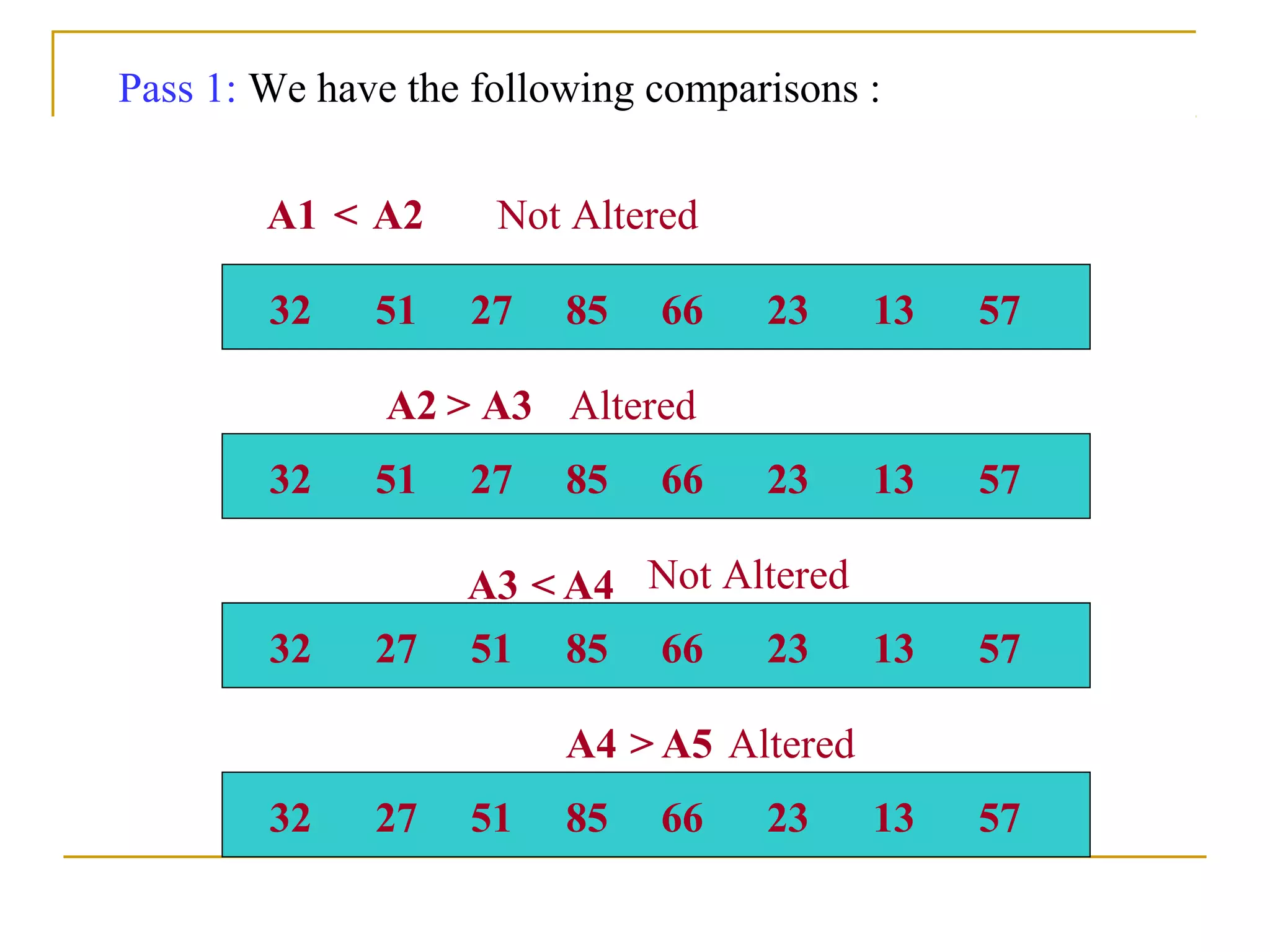
![3. Bubble Sort :
Suppose an array A with n elements A[1], A[2],…..,A[n] is in
memory. The bubble sort algo. For sorting A as follows:
Step 1: Compare A[1] and A[2] and arrange them in the desired
order, so that A[1] < A[2]. Then compare A[2] and A[3] and
arrange them so that A[2] < A[3]. Continue until we compare
A[N-1] with A[N] and arrange them.
Step 2: Repeat step 1 with one less comparison, that is, now we
stop after we compare and possibly rearrange A[N-1] and A[N-
1].
.
.
.](https://image.slidesharecdn.com/unit7-sorting-180714073502/85/Unit-7-sorting-11-320.jpg)
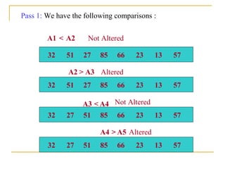
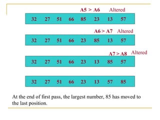
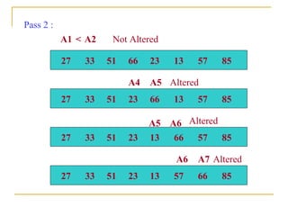
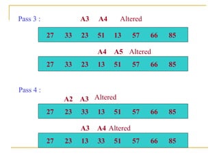
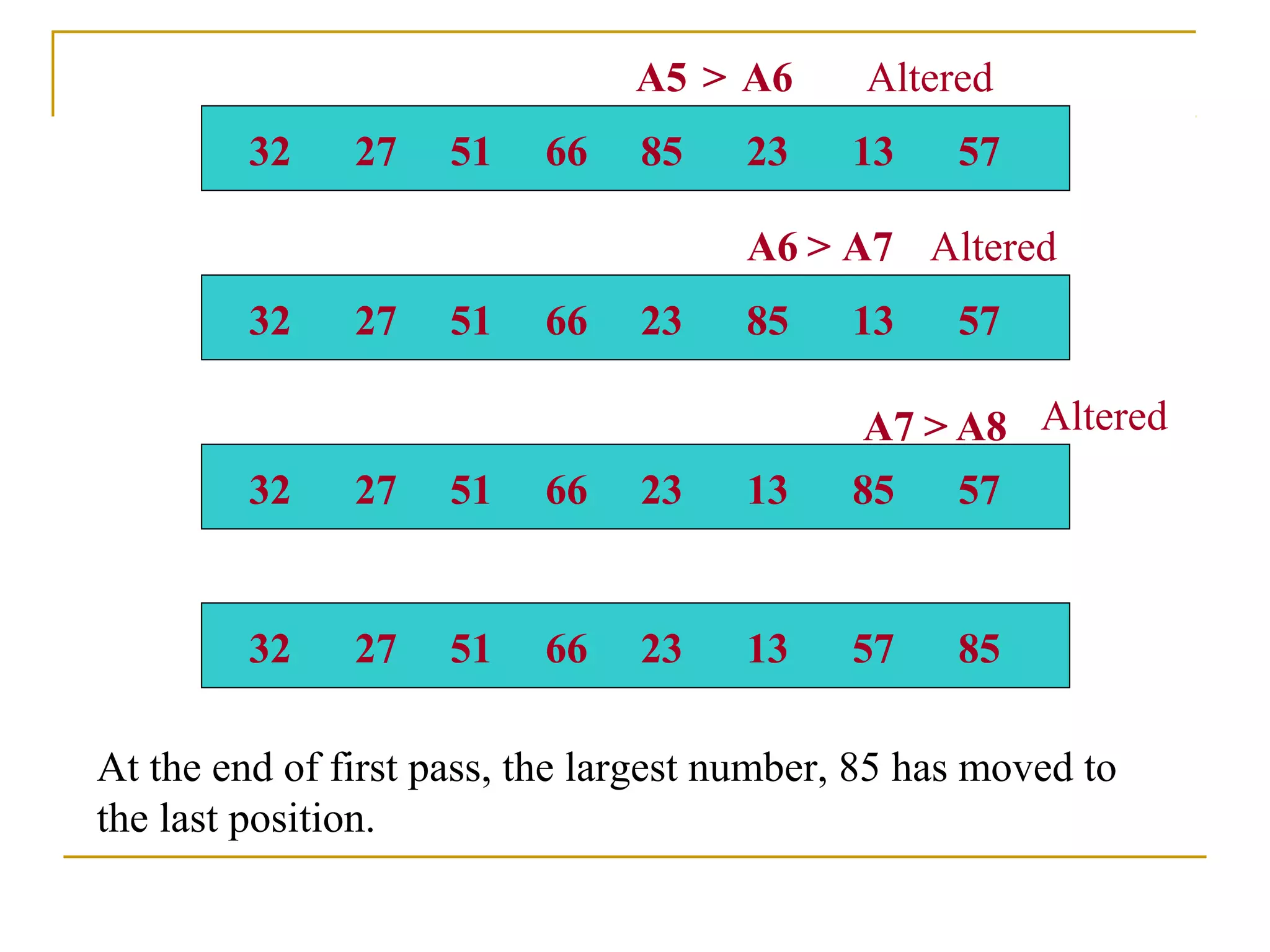
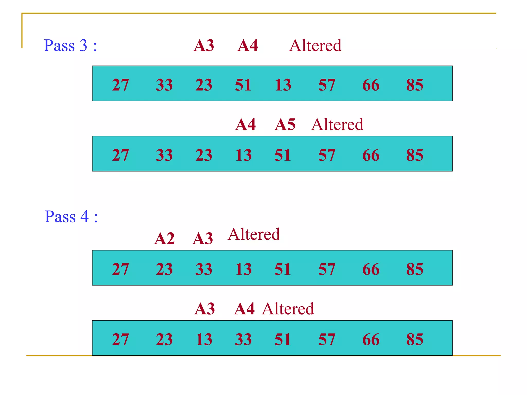
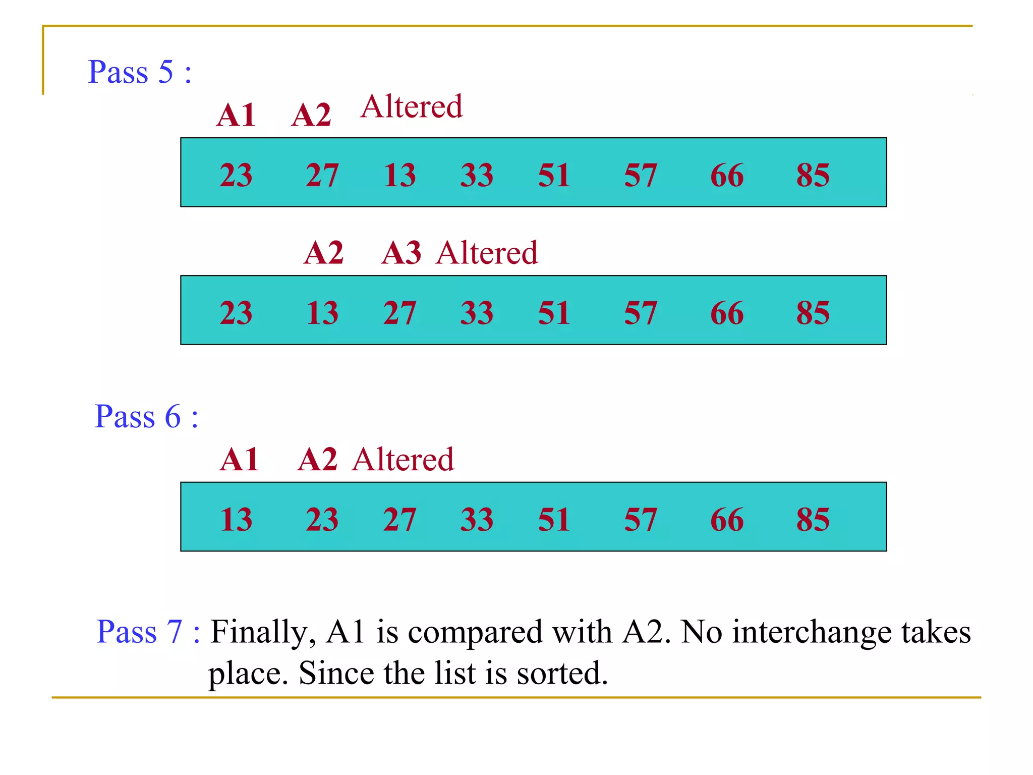
![Step N-1 : Compare A[1] with A[2] and arrange them so that
A[1] < A[2].
After N-1 steps, the list will be sorted in increasing order.
Suppose the following numbers are sorted in an array A :
32, 51, 27,85, 66, 23, 13, 57
We apply the bubble sort to the array A.](https://image.slidesharecdn.com/unit7-sorting-180714073502/85/Unit-7-sorting-12-320.jpg)
![BUBBLE(DATA, N)
Here DATA is an array with N elements. This algorithm sorts the
elements in DATA.
1. Repeat steps 2 and 3 for K = 1 to N-1.
2. Set PTR := 1. [ Initialize pass pointer PTR]
3. Repeat while PTR <= N – K: [Execute pass]
1. If DATA[PTR] > DATA[PTR + 1], then :
Interchange DATA[PTR] and DATA[PTR + 1]
[End of If structure]
2. Set PTR := PTR + 1.
[End of inner loop]
[End of step 1 outer loop]
4. Exit](https://image.slidesharecdn.com/unit7-sorting-180714073502/85/Unit-7-sorting-13-320.jpg)

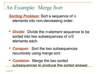
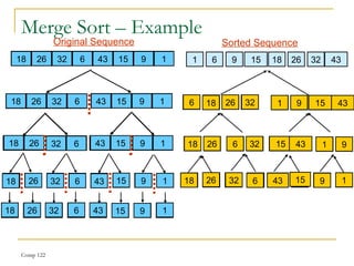
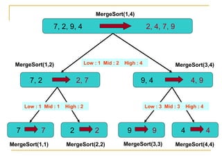
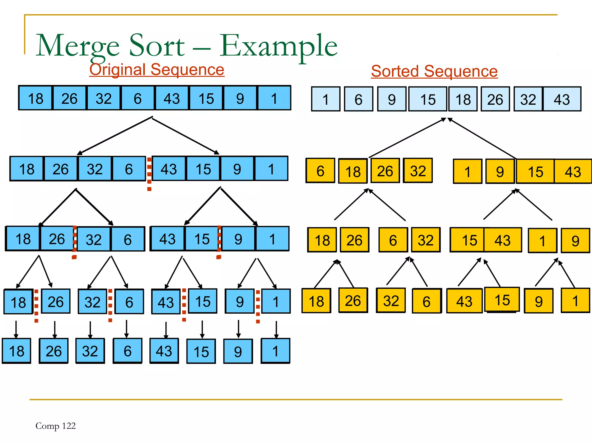
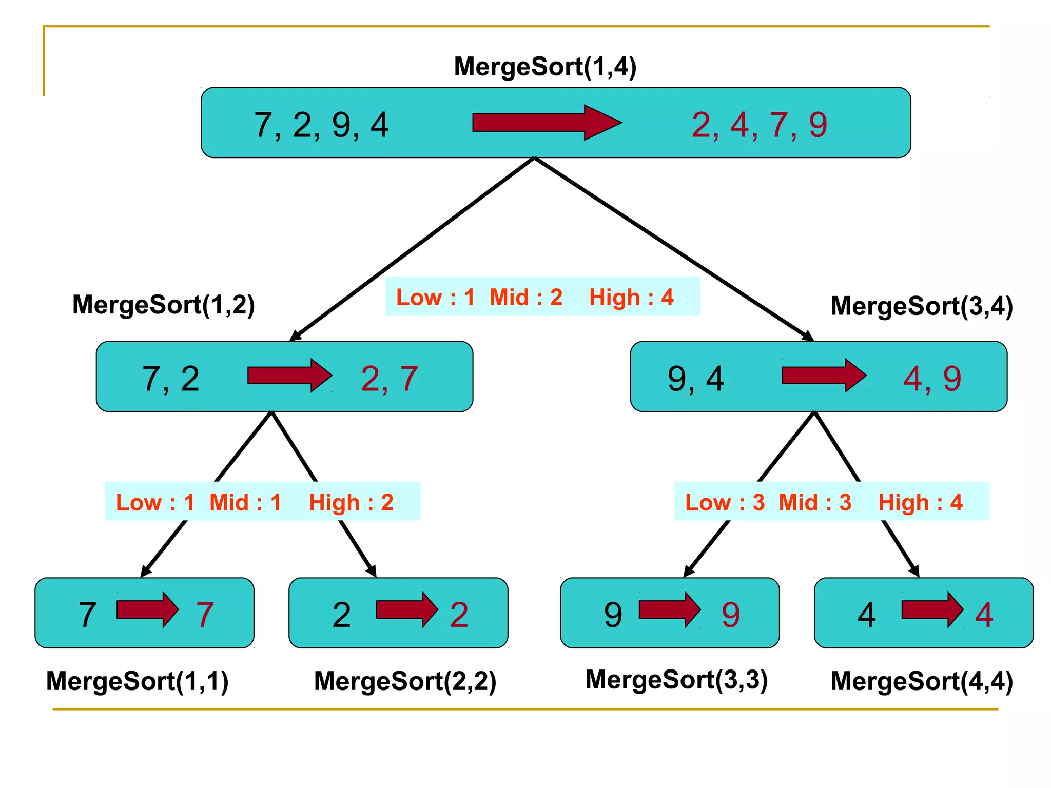
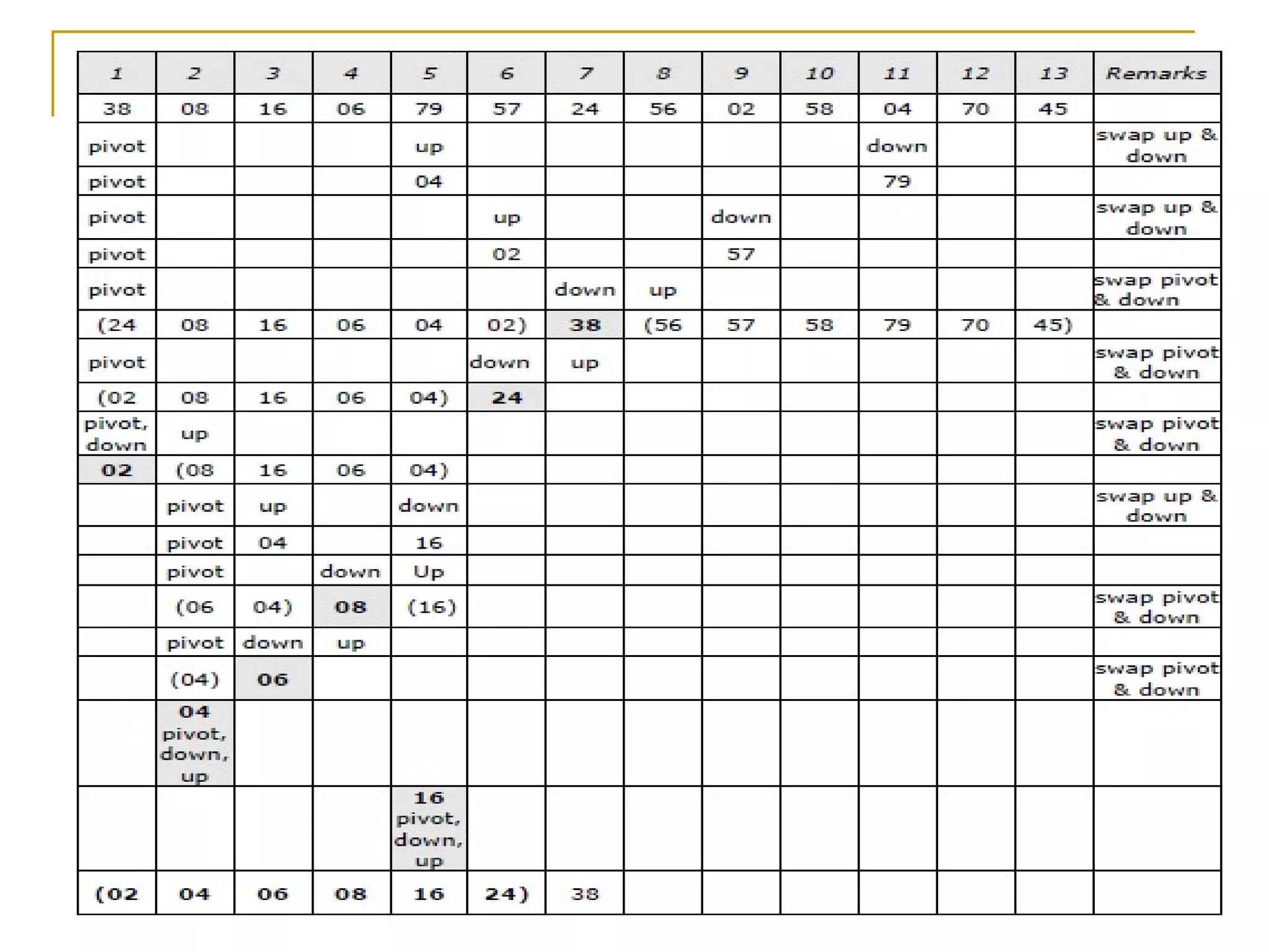
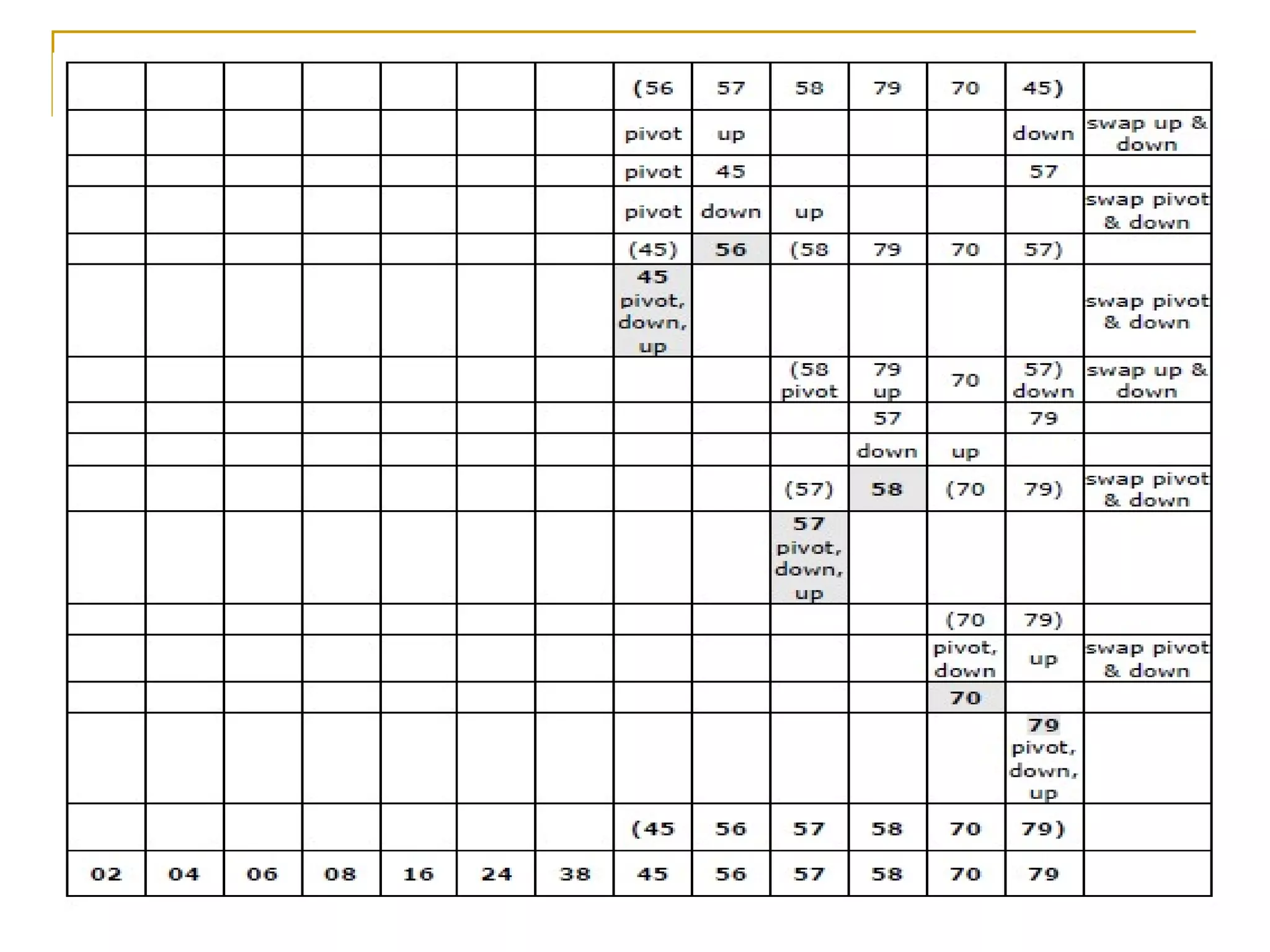
![4. Merge Sort :
Suppose an array A with n elements A[1], A[2],
…..,A[n] is in memory. The merge sort algorithm For
sorting A as follows:](https://image.slidesharecdn.com/unit7-sorting-180714073502/85/Unit-7-sorting-19-320.jpg)
![MERGESORT(LOW, HIGH)
1. Set LOW := 1.
2. If LOW < HIGH: then:
1. Set MID := (LOW + N)/2
2. Call MERGESORT(LOW, MID)
3. Call MERGESORT(MID+1, HIGH)
4. Call MERGE(LOW,MID,HIGH)
[End of step 2 loop]
7. Exit](https://image.slidesharecdn.com/unit7-sorting-180714073502/85/Unit-7-sorting-23-320.jpg)
![MERGE(A, LOW, MID, HIGH)
This algorithm merges two sorted sub arrays into one
array.
1. [Initialize]
h := LOW, i := LOW, j := MID + 1
2. Repeat while h <= MID && j <= HIGH:
If A[h] <= A[j] then:
Set b[i] := A[h]
Set h := h +1
ELSE:
Set b[i] := A[j]
Set j := j +1
[End of If structure]
Set i := i + 1
[End of loop]](https://image.slidesharecdn.com/unit7-sorting-180714073502/85/Unit-7-sorting-24-320.jpg)
![3. If h > MID then:
Set k := j
Repeat while k <= HIGH
Set h[i] := A[k]
Set i := i + 1
ELSE
Set k := h
Repeat while k <= MID
b[i] := a[k];
I := i+1;
4. Set k := LOW
Repeat while k <= HIGH
a[k] := b[k];
5. Return](https://image.slidesharecdn.com/unit7-sorting-180714073502/85/Unit-7-sorting-25-320.jpg)

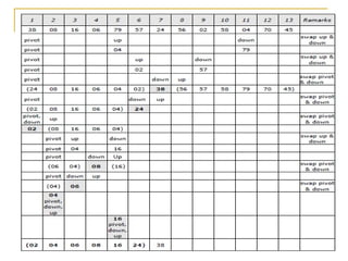
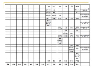

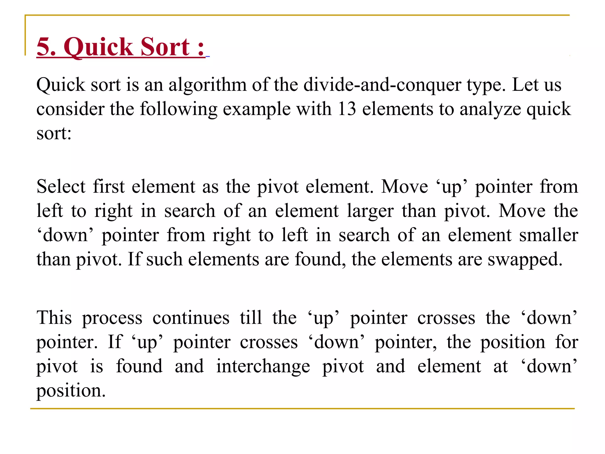
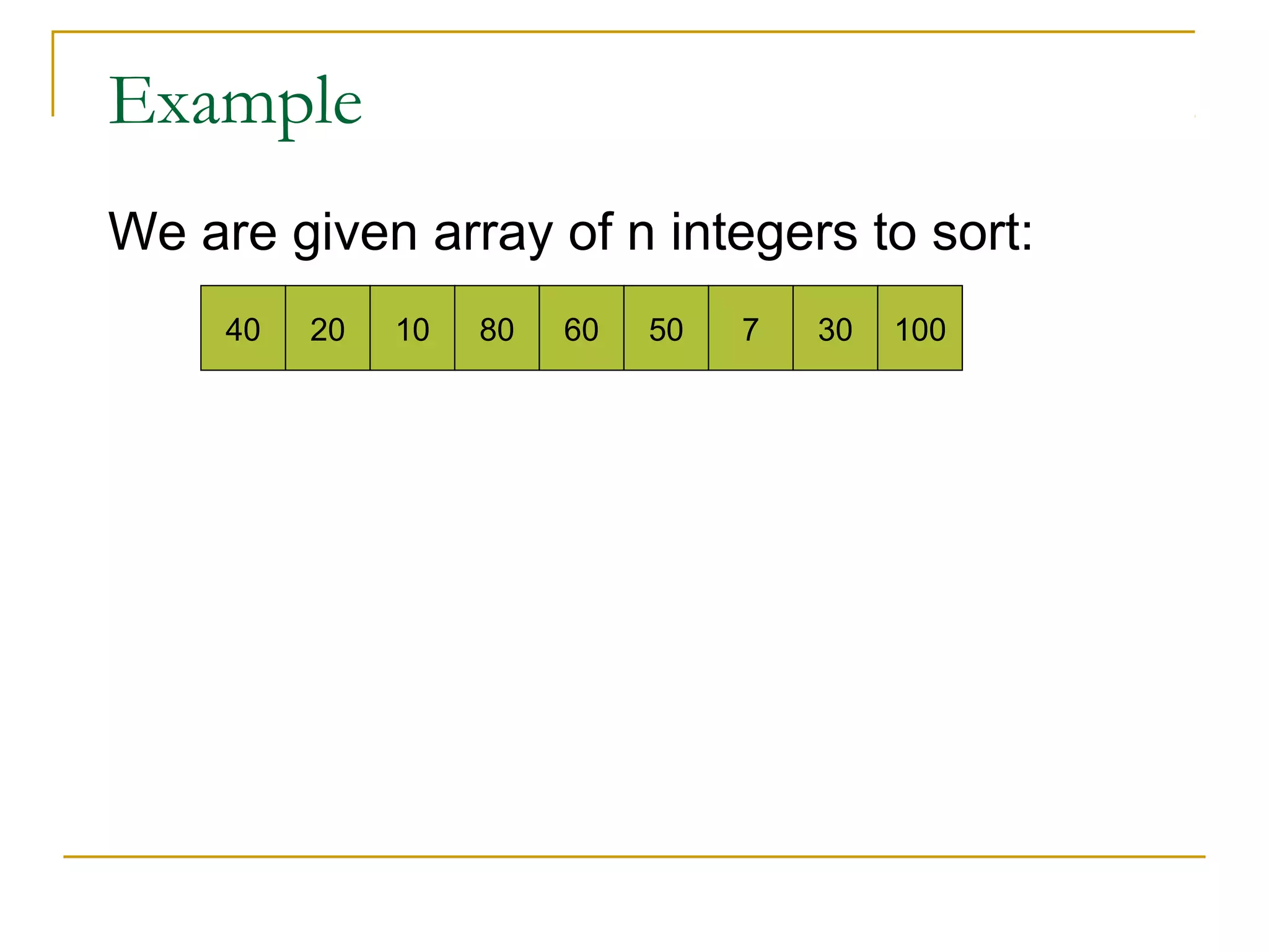
![40 20 10 80 60 50 7 30 100pivot_index = 0
[0] [1] [2] [3] [4] [5] [6] [7] [8]
i j](https://image.slidesharecdn.com/unit7-sorting-180714073502/85/Unit-7-sorting-36-320.jpg)
![40 20 10 80 60 50 7 30 100pivot_index = 0
[0] [1] [2] [3] [4] [5] [6] [7] [8]
i j
1. While data[i] <= data[pivot]
++i](https://image.slidesharecdn.com/unit7-sorting-180714073502/85/Unit-7-sorting-37-320.jpg)
![40 20 10 80 60 50 7 30 100pivot_index = 0
[0] [1] [2] [3] [4] [5] [6] [7] [8]
i j
1. While data[i] <= data[pivot]
++i](https://image.slidesharecdn.com/unit7-sorting-180714073502/85/Unit-7-sorting-38-320.jpg)
![40 20 10 80 60 50 7 30 100pivot_index = 0
[0] [1] [2] [3] [4] [5] [6] [7] [8]
i j
1. While data[i] <= data[pivot]
++i
2. While data[j] > data[pivot]
--j](https://image.slidesharecdn.com/unit7-sorting-180714073502/85/Unit-7-sorting-39-320.jpg)
![40 20 10 80 60 50 7 30 100pivot_index = 0
[0] [1] [2] [3] [4] [5] [6] [7] [8]
i j
1. While data[i] <= data[pivot]
++i
2. While data[j] > data[pivot]
--j](https://image.slidesharecdn.com/unit7-sorting-180714073502/85/Unit-7-sorting-40-320.jpg)
![40 20 10 80 60 50 7 30 100pivot_index = 0
[0] [1] [2] [3] [4] [5] [6] [7] [8]
i j
1. While data[i] <= data[pivot]
++i
2. While data[j] > data[pivot]
--j
3. If i < j
swap data[i] and data[j]](https://image.slidesharecdn.com/unit7-sorting-180714073502/85/Unit-7-sorting-41-320.jpg)
![40 20 10 30 60 50 7 80 100pivot_index = 0
i j
1. While data[i] <= data[pivot]
++i
2. While data[j] > data[pivot]
--j
3. If i < j
swap data[i] and data[j]
[0] [1] [2] [3] [4] [5] [6] [7] [8]](https://image.slidesharecdn.com/unit7-sorting-180714073502/85/Unit-7-sorting-42-320.jpg)
![40 20 10 30 60 50 7 80 100pivot_index = 0
i j
1. While data[i] <= data[pivot]
++i
2. While data[j] > data[pivot]
--j
3. If i < j
swap data[i] and data[j]
4. While j > i, go to 1.
[0] [1] [2] [3] [4] [5] [6] [7] [8]](https://image.slidesharecdn.com/unit7-sorting-180714073502/85/Unit-7-sorting-43-320.jpg)
![40 20 10 30 60 50 7 80 100pivot_index = 0
i j
1. While data[i] <= data[pivot]
++i
2. While data[j] > data[pivot]
--j
3. If i < j
swap data[i] and data[j]
4. While j > i, go to 1.
[0] [1] [2] [3] [4] [5] [6] [7] [8]](https://image.slidesharecdn.com/unit7-sorting-180714073502/85/Unit-7-sorting-44-320.jpg)
![40 20 10 30 60 50 7 80 100pivot_index = 0
i j
1. While data[i] <= data[pivot]
++i
2. While data[j] > data[pivot]
--j
3. If i < j
swap data[i] and data[j]
4. While j > i, go to 1.
[0] [1] [2] [3] [4] [5] [6] [7] [8]](https://image.slidesharecdn.com/unit7-sorting-180714073502/85/Unit-7-sorting-45-320.jpg)
![40 20 10 30 60 50 7 80 100pivot_index = 0
i j
1. While data[i] <= data[pivot]
++i
2. While data[j] > data[pivot]
--j
3. If i < j
swap data[i] and data[j]
4. While j > i, go to 1.
[0] [1] [2] [3] [4] [5] [6] [7] [8]](https://image.slidesharecdn.com/unit7-sorting-180714073502/85/Unit-7-sorting-46-320.jpg)
![40 20 10 30 60 50 7 80 100pivot_index = 0
i j
1. While data[i] <= data[pivot]
++i
2. While data[j] > data[pivot]
--j
3. If i < j
swap data[i] and data[j]
4. While j > i, go to 1.
[0] [1] [2] [3] [4] [5] [6] [7] [8]](https://image.slidesharecdn.com/unit7-sorting-180714073502/85/Unit-7-sorting-47-320.jpg)
![40 20 10 30 60 50 7 80 100pivot_index = 0
i j
1. While data[i] <= data[pivot]
++i
2. While data[j] > data[pivot]
--j
3. If i < j
swap data[i] and data[j]
4. While j > i, go to 1.
[0] [1] [2] [3] [4] [5] [6] [7] [8]](https://image.slidesharecdn.com/unit7-sorting-180714073502/85/Unit-7-sorting-48-320.jpg)
![1. While data[i] <= data[pivot]
++i
2. While data[j] > data[pivot]
--j
3. If i < j
swap data[i] and data[j]
4. While j > i, go to 1.
40 20 10 30 7 50 60 80 100pivot_index = 0
i j
[0] [1] [2] [3] [4] [5] [6] [7] [8]](https://image.slidesharecdn.com/unit7-sorting-180714073502/85/Unit-7-sorting-49-320.jpg)
![1. While data[i] <= data[pivot]
++i
2. While data[j] > data[pivot]
--j
3. If i < j
swap data[i] and data[j]
4. While j > i, go to 1.
40 20 10 30 7 50 60 80 100pivot_index = 0
i j
[0] [1] [2] [3] [4] [5] [6] [7] [8]](https://image.slidesharecdn.com/unit7-sorting-180714073502/85/Unit-7-sorting-50-320.jpg)
![1. While data[i] <= data[pivot]
++i
2. While data[j] > data[pivot]
--j
3. If i < j
swap data[i] and data[j]
4. While j > i, go to 1.
40 20 10 30 7 50 60 80 100pivot_index = 0
i j
[0] [1] [2] [3] [4] [5] [6] [7] [8]](https://image.slidesharecdn.com/unit7-sorting-180714073502/85/Unit-7-sorting-51-320.jpg)
![1. While data[i] <= data[pivot]
++i
2. While data[j] > data[pivot]
--j
3. If i < j
swap data[i] and data[j]
4. While j > i, go to 1.
40 20 10 30 7 50 60 80 100pivot_index = 0
i j
[0] [1] [2] [3] [4] [5] [6] [7] [8]](https://image.slidesharecdn.com/unit7-sorting-180714073502/85/Unit-7-sorting-52-320.jpg)
![1. While data[i] <= data[pivot]
++i
2. While data[j] > data[pivot]
--j
3. If i < j
swap data[i] and data[j]
4. While j > i, go to 1.
40 20 10 30 7 50 60 80 100pivot_index = 0
i j
[0] [1] [2] [3] [4] [5] [6] [7] [8]](https://image.slidesharecdn.com/unit7-sorting-180714073502/85/Unit-7-sorting-53-320.jpg)
![1. While data[i] <= data[pivot]
++i
2. While data[j] > data[pivot]
--j
3. If i < j
swap data[i] and data[j]
4. While j > i, go to 1.
40 20 10 30 7 50 60 80 100pivot_index = 0
i j
[0] [1] [2] [3] [4] [5] [6] [7] [8]](https://image.slidesharecdn.com/unit7-sorting-180714073502/85/Unit-7-sorting-54-320.jpg)
![1. While data[i] <= data[pivot]
++i
2. While data[j] > data[pivot]
--j
3. If i < j
swap data[i] and data[j]
4. While j > i, go to 1.
40 20 10 30 7 50 60 80 100pivot_index = 0
i j
[0] [1] [2] [3] [4] [5] [6] [7] [8]](https://image.slidesharecdn.com/unit7-sorting-180714073502/85/Unit-7-sorting-55-320.jpg)
![1. While data[i] <= data[pivot]
++i
2. While data[j] > data[pivot]
--j
3. If i < j
swap data[i] and data[j]
4. While j > i, go to 1.
40 20 10 30 7 50 60 80 100pivot_index = 0
i j
[0] [1] [2] [3] [4] [5] [6] [7] [8]](https://image.slidesharecdn.com/unit7-sorting-180714073502/85/Unit-7-sorting-56-320.jpg)
![1. While data[i] <= data[pivot]
++i
2. While data[j] > data[pivot]
--j
3. If i < j
swap data[i] and data[j]
4. While j > i, go to 1.
40 20 10 30 7 50 60 80 100pivot_index = 0
i j
[0] [1] [2] [3] [4] [5] [6] [7] [8]](https://image.slidesharecdn.com/unit7-sorting-180714073502/85/Unit-7-sorting-57-320.jpg)
![1. While data[i] <= data[pivot]
++i
2. While data[j] > data[pivot]
--j
3. If i < j
swap data[i] and data[j]
4. While j > i, go to 1.
5. Swap data[j] and data[pivot_index]
40 20 10 30 7 50 60 80 100pivot_index = 0
i j
[0] [1] [2] [3] [4] [5] [6] [7] [8]](https://image.slidesharecdn.com/unit7-sorting-180714073502/85/Unit-7-sorting-58-320.jpg)
![1. While data[i] <= data[pivot]
++i
2. While data[j] > data[pivot]
--j
3. If i < j
swap data[i] and data[j]
4. While j > i, go to 1.
5. Swap data[j] and data[pivot_index]
7 20 10 30 40 50 60 80 100pivot_index = 4
i j
[0] [1] [2] [3] [4] [5] [6] [7] [8]](https://image.slidesharecdn.com/unit7-sorting-180714073502/85/Unit-7-sorting-59-320.jpg)
![Partition Result
7 20 10 30 40 50 60 80 100
<= data[pivot] > data[pivot]
[0] [1] [2] [3] [4] [5] [6] [7] [8]](https://image.slidesharecdn.com/unit7-sorting-180714073502/85/Unit-7-sorting-60-320.jpg)
![Recursion: Quicksort Sub-arrays
7 20 10 30 40 50 60 80 100
<= data[pivot] > data[pivot]
[0] [1] [2] [3] [4] [5] [6] [7] [8]](https://image.slidesharecdn.com/unit7-sorting-180714073502/85/Unit-7-sorting-61-320.jpg)
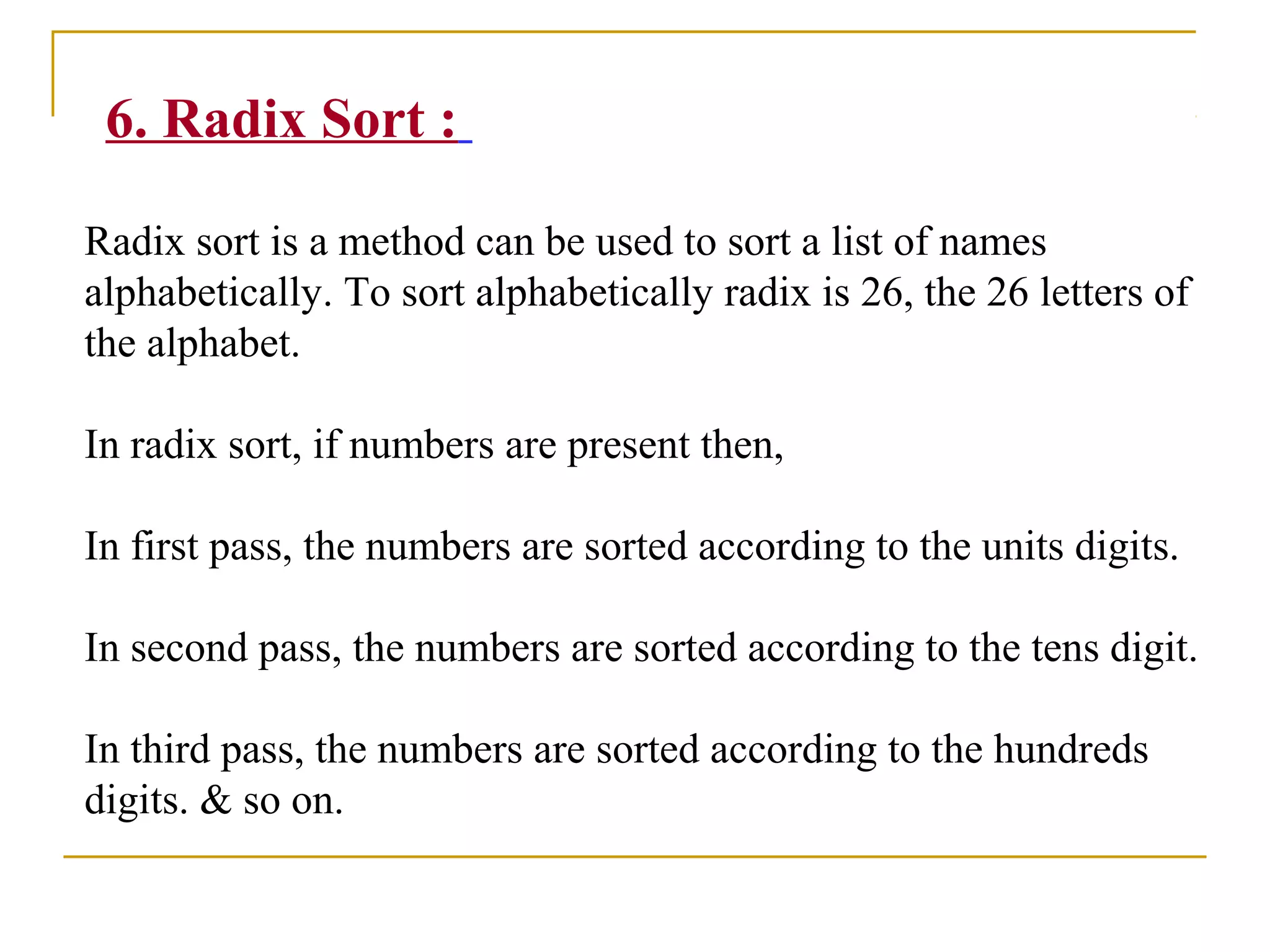
![radix_sort(int arr[], int n)
{
int bucket[10][5],buck[10],b[10];
int i,j,k,l,num,div,large,passes;
div=1;
num=0;
large=arr[0];
for(i=0 ; i< n ; i++)
{
if(arr[i] > large)
{
large = arr[i];
}
while(large > 0)
{
num++;
large = large/10;
}
for(passes=0 ; passes < num ;
passes++)
{
for(k=0 ; k< 10 ; k++)
{
buck[k] = 0;
}
for(i=0 ; i< n ;i++)
{
l = ((arr[i]/div)%10);
bucket[l][buck[l]++] = arr[i];
}
i=0;
for(k=0 ; k < 10 ; k++)
{
for(j=0 ; j < buck[k] ; j++)
{
arr[i++] = bucket[k][j];
}
}
div*=10;
}}}](https://image.slidesharecdn.com/unit7-sorting-180714073502/85/Unit-7-sorting-67-320.jpg)

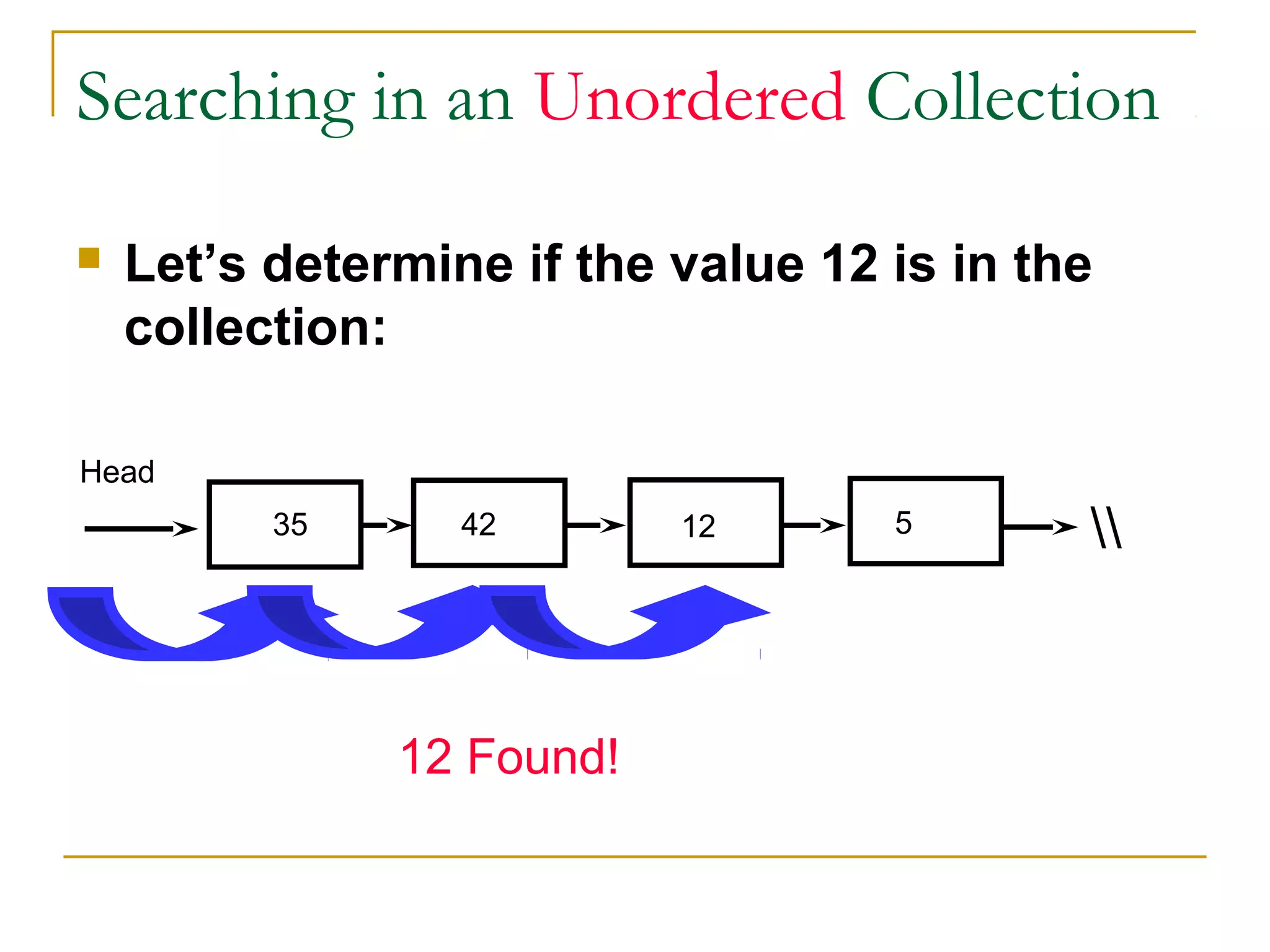
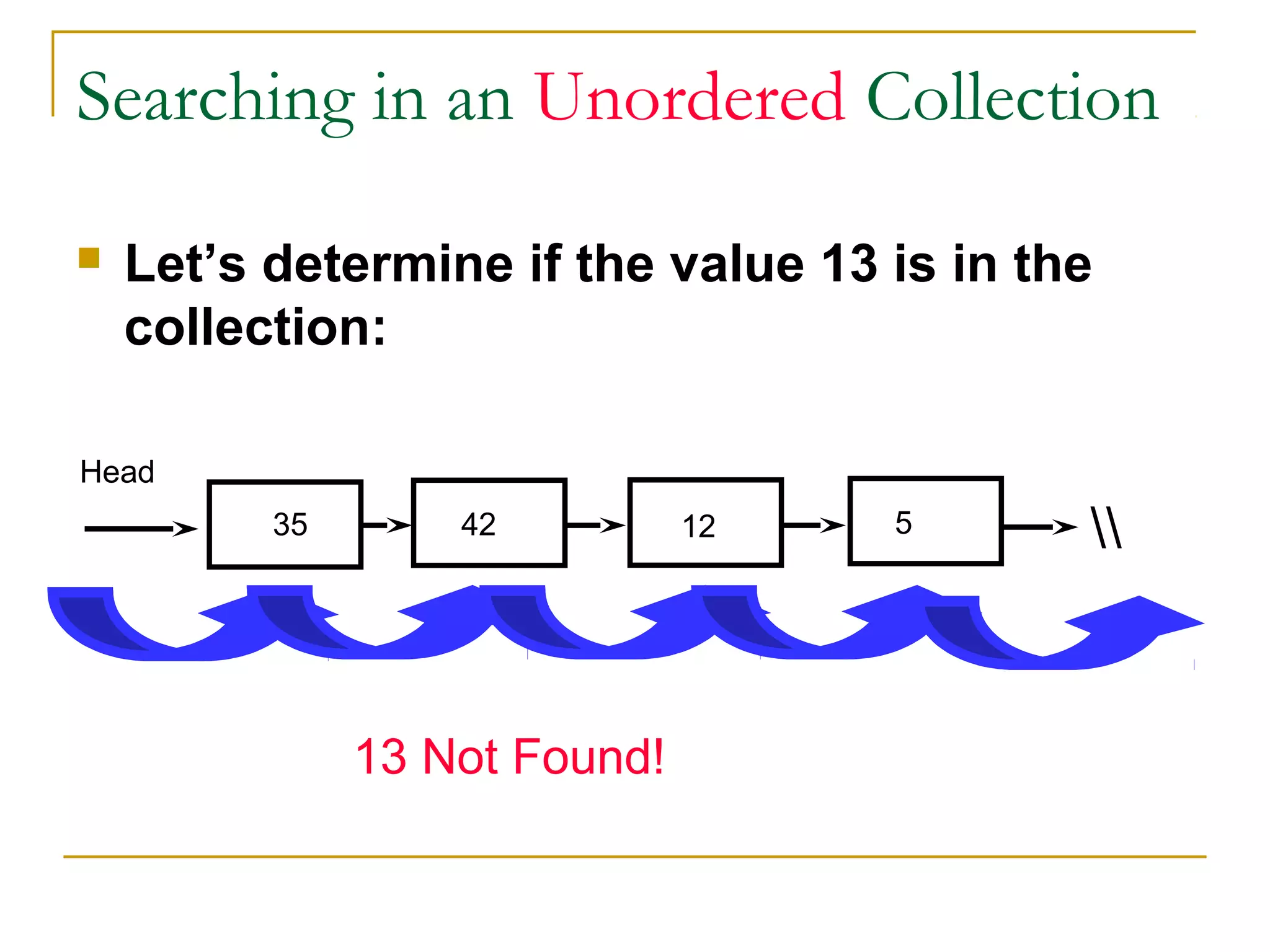
![Suppose there are ‘n’ elements organized sequentially on a
List.
The number of comparisons required to retrieve an element
from the list, purely depends on where the element is stored in
the list.
If it is the first element, one comparison will do; if it is second
element two comparisons are necessary and so on.
On an average you need [(n+1)/2] comparison’s to search an
element.
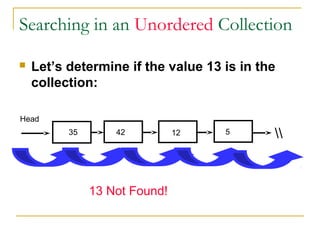
If search is not successful, you would need ’n’ comparisons.](https://image.slidesharecdn.com/unit7-sorting-180714073502/85/Unit-7-sorting-71-320.jpg)
![Algorithm
Linear Search ( Array A, Value x)
Step 1: Set i to 1
Step 2: if i > n then go to step 7
Step 3: if A[i] = x then go to step 6
Step 4: Set i to i + 1
Step 5: Go to Step 2
Step 6: Print Element x Found at index i and go to step 8
Step 7: Print element not found
Step 8: Exit](https://image.slidesharecdn.com/unit7-sorting-180714073502/85/Unit-7-sorting-72-320.jpg)

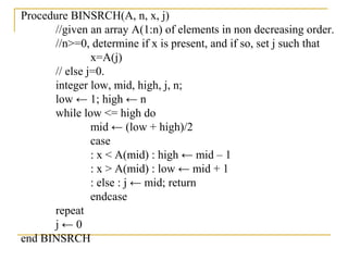
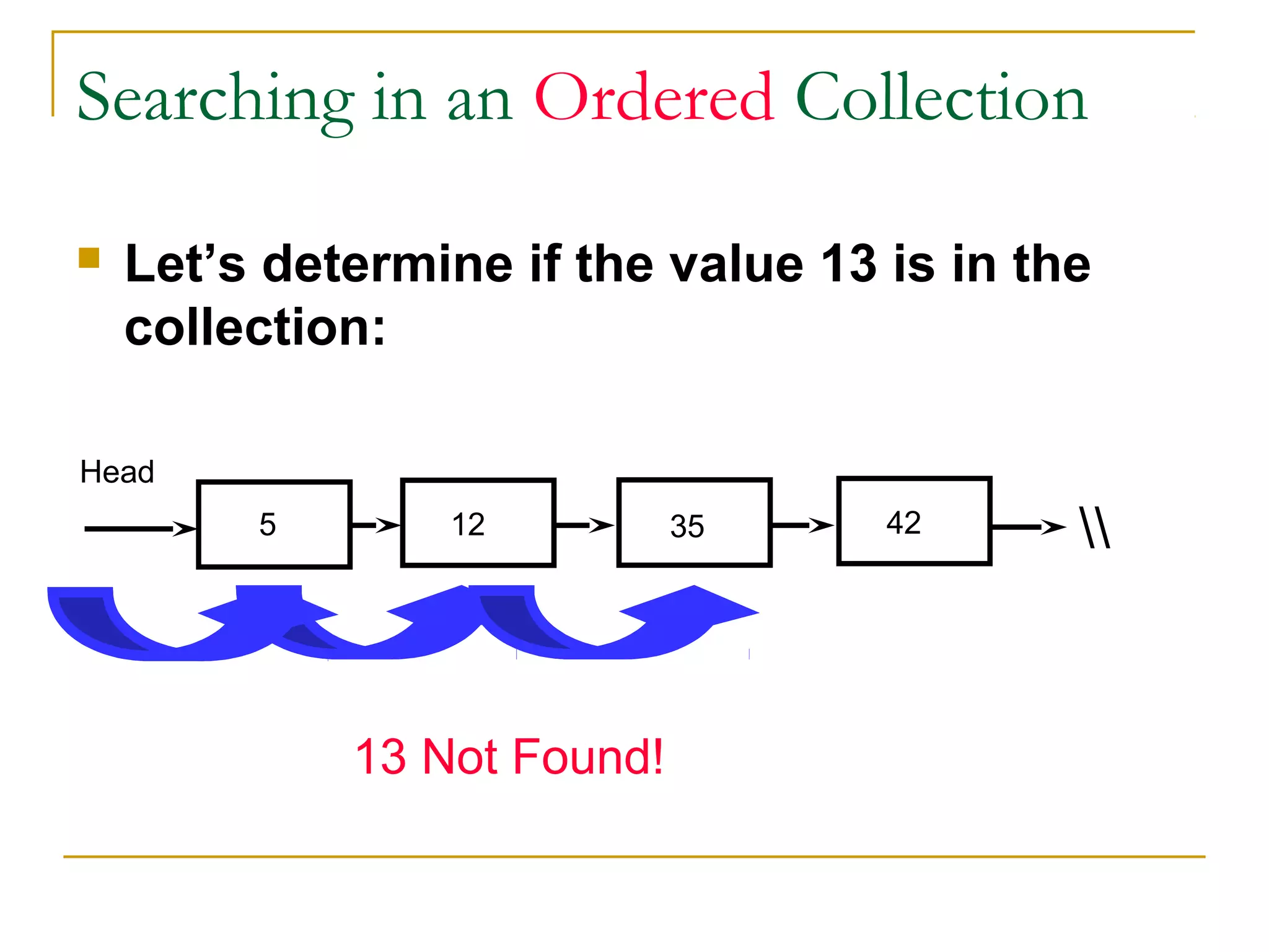
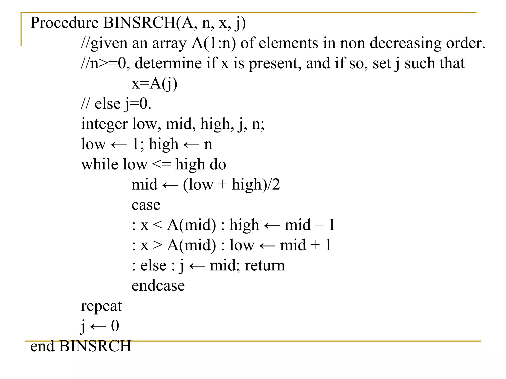
![2. BINARY SEARCH
If we have ‘n’ records which have been ordered by keys so that
x1 < x2 < … < xn .
When we are given a element ‘x’, binary search is used to find
the corresponding element from the list.
In case ‘x’ is present, we have to determine a value ‘j’ such that
a[j] = x(successful search).
If ‘x’ is not in the list then j is to set to zero (un successful
search).](https://image.slidesharecdn.com/unit7-sorting-180714073502/85/Unit-7-sorting-76-320.jpg)
![In Binary search we jump into the middle of the file, where we
find key a[mid], and compare ‘x’ with a[mid]. If x = a[mid] then
the desired record has been found.
If x < a[mid] then ‘x’ must be in that portion of the file that
precedes a[mid].
Similarly, if a[mid] > x, then further search is only necessary in
that part of the file which follows a[mid].](https://image.slidesharecdn.com/unit7-sorting-180714073502/85/Unit-7-sorting-77-320.jpg)
![Binary search (Example)
Example: Searching the array below for the value 42:
inde
x
0 1 2 3 4 5 6 7 8 9 1
0
1
1
1
2
1
3
1
4
1
5
16
valu
e
-4 2 7 1
0
1
5
2
0
2
2
2
5
3
0
3
6
4
2
5
0
5
6
6
8
8
5
9
2
10
3
min mid max
Check A[mid]== number If yes PRINT
Check number<A[mid]
Check number>A[mid]
If yes min=mid+1
and repeat
If yes max=mid-1
and repeat](https://image.slidesharecdn.com/unit7-sorting-180714073502/85/Unit-7-sorting-79-320.jpg)

![1.Insertion Sort :
Suppose an array A with n elements A[1], A[2],…..,A[n] is in
memory. The insertion sort algorithm. Scans A from A[1] to A[n],
inserting each element A[K] into its proper position in the
previously sorted sub array A[1], A[2], …,A[K-1]. That is:
Pass 1: A[1] by itself is trivially sorted.
Pass 2: A[2] is inserted either before or after A[1] so that A[1], A[2]
is sorted.
Pass 3: A[3] is inserted into its proper place in A[1], A[2], that is
before A[1], between A[1] and A[2], or after A[2], So that
A[1], A[2],A[3] is sorted.](https://image.slidesharecdn.com/unit7-sorting-180714073502/75/Unit-7-sorting-3-2048.jpg)
![Pass 4: A[4] is inserted into its proper place in A[1],A[2],A[3]
so that:
A[1],A[2],A[3],A[4] is sorted.
.
.
.
.
.
Pass N : A[N] is inserted into its proper place in
A[1],A[2],…,A[N-1] so that :
A[1],A[2],……,A[N] is sorted.](https://image.slidesharecdn.com/unit7-sorting-180714073502/75/Unit-7-sorting-4-2048.jpg)
![Algorithm :
INSERTION(A,N)
1. Set A[0] := -∞ [Initializes element]
2. Repeat Steps 3 to 5 for K = 2,3,…..,N:
3. Set TEMP := A[K] and PTR := K-1
4. Repeat while TEMP < A[PTR]:
1. Set A[PTR + 1] := A[PTR]. [Moves element
forward.]
2. Set PTR := PTR – 1
5. Set A[PTR + 1] := TEMP [Inserts element in proper
place.]
[End of Step 2 loop.]
6. Return](https://image.slidesharecdn.com/unit7-sorting-180714073502/75/Unit-7-sorting-5-2048.jpg)
![Pass A[0] A[1] A[2] A[3] A[4] A[5] A[6] A[7] A[8]
K=1: -∞ 33 44 11 88 22 66 55
K=2: -∞ 77 33 44 11 88 22 66 55
K=3: -∞ 33 77 44 11 88 22 66 55
K=4: -∞ 33 44 77 11 88 22 66 55
K=5: -∞ 11 33 44 77 88 22 66 55
K=6: -∞ 11 33 44 77 88 22 66 55
K=7: -∞ 11 22 33 44 77 88 66 55
K=8: -∞ 11 22 33 44 66 77 88 55
Sorted: -∞ 11 22 33 44 55 66 77 88
Array A is, 77, 33, 44, 11, 88, 22, 66, 55
77](https://image.slidesharecdn.com/unit7-sorting-180714073502/75/Unit-7-sorting-6-2048.jpg)
![2. Selection Sort :
Suppose an array A with n elements A[1], A[2],…..,A[n] is in
memory. The selection sort algo. For sorting A as follows:
Pass 1: Find the location LOC of the smallest in the list of N elements
A[1],A[2],….,A[N], and then interchange A[LOC] and A[1],
Then : A[1] is sorted.
Pass 2: Find the location LOC of the smallest in the sublist of N-1
elements A[1],A[2],….,A[N], and then interchange A[LOC]
and A[2], Then : A[1], A[2]is sorted. Since A[1] <= A[2].
Pass 3:Find the location LOC of the smallest in the sub list of N-2
elements A[1],A[2],….,A[N], and then interchange A[LOC]
and A[3], Then : A[1], A[2],A[3]is sorted. Since A[2] <= A[3].](https://image.slidesharecdn.com/unit7-sorting-180714073502/75/Unit-7-sorting-7-2048.jpg)
![.
.
.
Pass N-1:Find the location LOC of the smaller of the elements
A[N-1],A[N], and then interchange A[LOC] and A[N-
1], Then : A[1],A[2],….A[N]is sorted.
Since A[N-1] <= A[N].
Thus A is sorted after N-1 passes.](https://image.slidesharecdn.com/unit7-sorting-180714073502/75/Unit-7-sorting-8-2048.jpg)
![Algorithm :
SELECTION(A,N)
1. Repeat Steps 2 and 3 for K=1,2,….,N-1
2. Call Min (A,K,N,LOC)
3. [Interchange A[K] and A[LOC]]
Set TEMP := A[K], A[K] := A{LOC] and A[LOC] :=
TEMP
[End of step 1 loop]
4. Exit
MIN(A,K,N,LOC)
1. Set MIN := A[K] and LOC := K. [Initialize pointers]
2. Repeat for J=K+1,K+2,….,N
If MIN > A[J], then :
Set MIN := A[J] and LOC := A[J] and LOC := J
[End of loop]
3. Return](https://image.slidesharecdn.com/unit7-sorting-180714073502/75/Unit-7-sorting-9-2048.jpg)
![Pass A[1] A[2] A[3] A[4] A[5] A[6] A[7] A[8]
K=1:
LOC=4
33 44 11 88 22 66 55
K=2:
LOC=6
11 33 44 77 88 22 66 55
K=3:
LOC=6
11 22 44 77 88 33 66 55
K=4:
LOC=6
11 22 33 77 88 44 66 55
K=5:
LOC=8
11 22 33 44 88 77 66 55
K=6:
LOC=7
11 22 33 44 55 77 66 88
K=7:
LOC=7
11 22 33 44 55 66 77 88
Sorted: 11 22 33 44 55 66 77 88
Array A is, 77, 33, 44, 11, 88, 22, 66, 55
77](https://image.slidesharecdn.com/unit7-sorting-180714073502/75/Unit-7-sorting-10-2048.jpg)
![3. Bubble Sort :
Suppose an array A with n elements A[1], A[2],…..,A[n] is in
memory. The bubble sort algo. For sorting A as follows:
Step 1: Compare A[1] and A[2] and arrange them in the desired
order, so that A[1] < A[2]. Then compare A[2] and A[3] and
arrange them so that A[2] < A[3]. Continue until we compare
A[N-1] with A[N] and arrange them.
Step 2: Repeat step 1 with one less comparison, that is, now we
stop after we compare and possibly rearrange A[N-1] and A[N-
1].
.
.
.](https://image.slidesharecdn.com/unit7-sorting-180714073502/75/Unit-7-sorting-11-2048.jpg)
![Step N-1 : Compare A[1] with A[2] and arrange them so that
A[1] < A[2].
After N-1 steps, the list will be sorted in increasing order.
Suppose the following numbers are sorted in an array A :
32, 51, 27,85, 66, 23, 13, 57
We apply the bubble sort to the array A.](https://image.slidesharecdn.com/unit7-sorting-180714073502/75/Unit-7-sorting-12-2048.jpg)
![BUBBLE(DATA, N)
Here DATA is an array with N elements. This algorithm sorts the
elements in DATA.
1. Repeat steps 2 and 3 for K = 1 to N-1.
2. Set PTR := 1. [ Initialize pass pointer PTR]
3. Repeat while PTR <= N – K: [Execute pass]
1. If DATA[PTR] > DATA[PTR + 1], then :
Interchange DATA[PTR] and DATA[PTR + 1]
[End of If structure]
2. Set PTR := PTR + 1.
[End of inner loop]
[End of step 1 outer loop]
4. Exit](https://image.slidesharecdn.com/unit7-sorting-180714073502/75/Unit-7-sorting-13-2048.jpg)
![4. Merge Sort :
Suppose an array A with n elements A[1], A[2],
…..,A[n] is in memory. The merge sort algorithm For
sorting A as follows:](https://image.slidesharecdn.com/unit7-sorting-180714073502/75/Unit-7-sorting-19-2048.jpg)

![MERGESORT(LOW, HIGH)
1. Set LOW := 1.
2. If LOW < HIGH: then:
1. Set MID := (LOW + N)/2
2. Call MERGESORT(LOW, MID)
3. Call MERGESORT(MID+1, HIGH)
4. Call MERGE(LOW,MID,HIGH)
[End of step 2 loop]
7. Exit](https://image.slidesharecdn.com/unit7-sorting-180714073502/75/Unit-7-sorting-23-2048.jpg)
![MERGE(A, LOW, MID, HIGH)
This algorithm merges two sorted sub arrays into one
array.
1. [Initialize]
h := LOW, i := LOW, j := MID + 1
2. Repeat while h <= MID && j <= HIGH:
If A[h] <= A[j] then:
Set b[i] := A[h]
Set h := h +1
ELSE:
Set b[i] := A[j]
Set j := j +1
[End of If structure]
Set i := i + 1
[End of loop]](https://image.slidesharecdn.com/unit7-sorting-180714073502/75/Unit-7-sorting-24-2048.jpg)
![3. If h > MID then:
Set k := j
Repeat while k <= HIGH
Set h[i] := A[k]
Set i := i + 1
ELSE
Set k := h
Repeat while k <= MID
b[i] := a[k];
I := i+1;
4. Set k := LOW
Repeat while k <= HIGH
a[k] := b[k];
5. Return](https://image.slidesharecdn.com/unit7-sorting-180714073502/75/Unit-7-sorting-25-2048.jpg)

![40 20 10 80 60 50 7 30 100pivot_index = 0
[0] [1] [2] [3] [4] [5] [6] [7] [8]
i j](https://image.slidesharecdn.com/unit7-sorting-180714073502/75/Unit-7-sorting-36-2048.jpg)
![40 20 10 80 60 50 7 30 100pivot_index = 0
[0] [1] [2] [3] [4] [5] [6] [7] [8]
i j
1. While data[i] <= data[pivot]
++i](https://image.slidesharecdn.com/unit7-sorting-180714073502/75/Unit-7-sorting-37-2048.jpg)
![40 20 10 80 60 50 7 30 100pivot_index = 0
[0] [1] [2] [3] [4] [5] [6] [7] [8]
i j
1. While data[i] <= data[pivot]
++i](https://image.slidesharecdn.com/unit7-sorting-180714073502/75/Unit-7-sorting-38-2048.jpg)
![40 20 10 80 60 50 7 30 100pivot_index = 0
[0] [1] [2] [3] [4] [5] [6] [7] [8]
i j
1. While data[i] <= data[pivot]
++i
2. While data[j] > data[pivot]
--j](https://image.slidesharecdn.com/unit7-sorting-180714073502/75/Unit-7-sorting-39-2048.jpg)
![40 20 10 80 60 50 7 30 100pivot_index = 0
[0] [1] [2] [3] [4] [5] [6] [7] [8]
i j
1. While data[i] <= data[pivot]
++i
2. While data[j] > data[pivot]
--j](https://image.slidesharecdn.com/unit7-sorting-180714073502/75/Unit-7-sorting-40-2048.jpg)
![40 20 10 80 60 50 7 30 100pivot_index = 0
[0] [1] [2] [3] [4] [5] [6] [7] [8]
i j
1. While data[i] <= data[pivot]
++i
2. While data[j] > data[pivot]
--j
3. If i < j
swap data[i] and data[j]](https://image.slidesharecdn.com/unit7-sorting-180714073502/75/Unit-7-sorting-41-2048.jpg)
![40 20 10 30 60 50 7 80 100pivot_index = 0
i j
1. While data[i] <= data[pivot]
++i
2. While data[j] > data[pivot]
--j
3. If i < j
swap data[i] and data[j]
[0] [1] [2] [3] [4] [5] [6] [7] [8]](https://image.slidesharecdn.com/unit7-sorting-180714073502/75/Unit-7-sorting-42-2048.jpg)
![40 20 10 30 60 50 7 80 100pivot_index = 0
i j
1. While data[i] <= data[pivot]
++i
2. While data[j] > data[pivot]
--j
3. If i < j
swap data[i] and data[j]
4. While j > i, go to 1.
[0] [1] [2] [3] [4] [5] [6] [7] [8]](https://image.slidesharecdn.com/unit7-sorting-180714073502/75/Unit-7-sorting-43-2048.jpg)
![40 20 10 30 60 50 7 80 100pivot_index = 0
i j
1. While data[i] <= data[pivot]
++i
2. While data[j] > data[pivot]
--j
3. If i < j
swap data[i] and data[j]
4. While j > i, go to 1.
[0] [1] [2] [3] [4] [5] [6] [7] [8]](https://image.slidesharecdn.com/unit7-sorting-180714073502/75/Unit-7-sorting-44-2048.jpg)
![40 20 10 30 60 50 7 80 100pivot_index = 0
i j
1. While data[i] <= data[pivot]
++i
2. While data[j] > data[pivot]
--j
3. If i < j
swap data[i] and data[j]
4. While j > i, go to 1.
[0] [1] [2] [3] [4] [5] [6] [7] [8]](https://image.slidesharecdn.com/unit7-sorting-180714073502/75/Unit-7-sorting-45-2048.jpg)
![40 20 10 30 60 50 7 80 100pivot_index = 0
i j
1. While data[i] <= data[pivot]
++i
2. While data[j] > data[pivot]
--j
3. If i < j
swap data[i] and data[j]
4. While j > i, go to 1.
[0] [1] [2] [3] [4] [5] [6] [7] [8]](https://image.slidesharecdn.com/unit7-sorting-180714073502/75/Unit-7-sorting-46-2048.jpg)
![40 20 10 30 60 50 7 80 100pivot_index = 0
i j
1. While data[i] <= data[pivot]
++i
2. While data[j] > data[pivot]
--j
3. If i < j
swap data[i] and data[j]
4. While j > i, go to 1.
[0] [1] [2] [3] [4] [5] [6] [7] [8]](https://image.slidesharecdn.com/unit7-sorting-180714073502/75/Unit-7-sorting-47-2048.jpg)
![40 20 10 30 60 50 7 80 100pivot_index = 0
i j
1. While data[i] <= data[pivot]
++i
2. While data[j] > data[pivot]
--j
3. If i < j
swap data[i] and data[j]
4. While j > i, go to 1.
[0] [1] [2] [3] [4] [5] [6] [7] [8]](https://image.slidesharecdn.com/unit7-sorting-180714073502/75/Unit-7-sorting-48-2048.jpg)
![1. While data[i] <= data[pivot]
++i
2. While data[j] > data[pivot]
--j
3. If i < j
swap data[i] and data[j]
4. While j > i, go to 1.
40 20 10 30 7 50 60 80 100pivot_index = 0
i j
[0] [1] [2] [3] [4] [5] [6] [7] [8]](https://image.slidesharecdn.com/unit7-sorting-180714073502/75/Unit-7-sorting-49-2048.jpg)
![1. While data[i] <= data[pivot]
++i
2. While data[j] > data[pivot]
--j
3. If i < j
swap data[i] and data[j]
4. While j > i, go to 1.
40 20 10 30 7 50 60 80 100pivot_index = 0
i j
[0] [1] [2] [3] [4] [5] [6] [7] [8]](https://image.slidesharecdn.com/unit7-sorting-180714073502/75/Unit-7-sorting-50-2048.jpg)
![1. While data[i] <= data[pivot]
++i
2. While data[j] > data[pivot]
--j
3. If i < j
swap data[i] and data[j]
4. While j > i, go to 1.
40 20 10 30 7 50 60 80 100pivot_index = 0
i j
[0] [1] [2] [3] [4] [5] [6] [7] [8]](https://image.slidesharecdn.com/unit7-sorting-180714073502/75/Unit-7-sorting-51-2048.jpg)
![1. While data[i] <= data[pivot]
++i
2. While data[j] > data[pivot]
--j
3. If i < j
swap data[i] and data[j]
4. While j > i, go to 1.
40 20 10 30 7 50 60 80 100pivot_index = 0
i j
[0] [1] [2] [3] [4] [5] [6] [7] [8]](https://image.slidesharecdn.com/unit7-sorting-180714073502/75/Unit-7-sorting-52-2048.jpg)
![1. While data[i] <= data[pivot]
++i
2. While data[j] > data[pivot]
--j
3. If i < j
swap data[i] and data[j]
4. While j > i, go to 1.
40 20 10 30 7 50 60 80 100pivot_index = 0
i j
[0] [1] [2] [3] [4] [5] [6] [7] [8]](https://image.slidesharecdn.com/unit7-sorting-180714073502/75/Unit-7-sorting-53-2048.jpg)
![1. While data[i] <= data[pivot]
++i
2. While data[j] > data[pivot]
--j
3. If i < j
swap data[i] and data[j]
4. While j > i, go to 1.
40 20 10 30 7 50 60 80 100pivot_index = 0
i j
[0] [1] [2] [3] [4] [5] [6] [7] [8]](https://image.slidesharecdn.com/unit7-sorting-180714073502/75/Unit-7-sorting-54-2048.jpg)
![1. While data[i] <= data[pivot]
++i
2. While data[j] > data[pivot]
--j
3. If i < j
swap data[i] and data[j]
4. While j > i, go to 1.
40 20 10 30 7 50 60 80 100pivot_index = 0
i j
[0] [1] [2] [3] [4] [5] [6] [7] [8]](https://image.slidesharecdn.com/unit7-sorting-180714073502/75/Unit-7-sorting-55-2048.jpg)
![1. While data[i] <= data[pivot]
++i
2. While data[j] > data[pivot]
--j
3. If i < j
swap data[i] and data[j]
4. While j > i, go to 1.
40 20 10 30 7 50 60 80 100pivot_index = 0
i j
[0] [1] [2] [3] [4] [5] [6] [7] [8]](https://image.slidesharecdn.com/unit7-sorting-180714073502/75/Unit-7-sorting-56-2048.jpg)
![1. While data[i] <= data[pivot]
++i
2. While data[j] > data[pivot]
--j
3. If i < j
swap data[i] and data[j]
4. While j > i, go to 1.
40 20 10 30 7 50 60 80 100pivot_index = 0
i j
[0] [1] [2] [3] [4] [5] [6] [7] [8]](https://image.slidesharecdn.com/unit7-sorting-180714073502/75/Unit-7-sorting-57-2048.jpg)
![1. While data[i] <= data[pivot]
++i
2. While data[j] > data[pivot]
--j
3. If i < j
swap data[i] and data[j]
4. While j > i, go to 1.
5. Swap data[j] and data[pivot_index]
40 20 10 30 7 50 60 80 100pivot_index = 0
i j
[0] [1] [2] [3] [4] [5] [6] [7] [8]](https://image.slidesharecdn.com/unit7-sorting-180714073502/75/Unit-7-sorting-58-2048.jpg)
![1. While data[i] <= data[pivot]
++i
2. While data[j] > data[pivot]
--j
3. If i < j
swap data[i] and data[j]
4. While j > i, go to 1.
5. Swap data[j] and data[pivot_index]
7 20 10 30 40 50 60 80 100pivot_index = 4
i j
[0] [1] [2] [3] [4] [5] [6] [7] [8]](https://image.slidesharecdn.com/unit7-sorting-180714073502/75/Unit-7-sorting-59-2048.jpg)
![Partition Result
7 20 10 30 40 50 60 80 100
<= data[pivot] > data[pivot]
[0] [1] [2] [3] [4] [5] [6] [7] [8]](https://image.slidesharecdn.com/unit7-sorting-180714073502/75/Unit-7-sorting-60-2048.jpg)
![Recursion: Quicksort Sub-arrays
7 20 10 30 40 50 60 80 100
<= data[pivot] > data[pivot]
[0] [1] [2] [3] [4] [5] [6] [7] [8]](https://image.slidesharecdn.com/unit7-sorting-180714073502/75/Unit-7-sorting-61-2048.jpg)
![radix_sort(int arr[], int n)
{
int bucket[10][5],buck[10],b[10];
int i,j,k,l,num,div,large,passes;
div=1;
num=0;
large=arr[0];
for(i=0 ; i< n ; i++)
{
if(arr[i] > large)
{
large = arr[i];
}
while(large > 0)
{
num++;
large = large/10;
}
for(passes=0 ; passes < num ;
passes++)
{
for(k=0 ; k< 10 ; k++)
{
buck[k] = 0;
}
for(i=0 ; i< n ;i++)
{
l = ((arr[i]/div)%10);
bucket[l][buck[l]++] = arr[i];
}
i=0;
for(k=0 ; k < 10 ; k++)
{
for(j=0 ; j < buck[k] ; j++)
{
arr[i++] = bucket[k][j];
}
}
div*=10;
}}}](https://image.slidesharecdn.com/unit7-sorting-180714073502/75/Unit-7-sorting-67-2048.jpg)
![Suppose there are ‘n’ elements organized sequentially on a
List.
The number of comparisons required to retrieve an element
from the list, purely depends on where the element is stored in
the list.
If it is the first element, one comparison will do; if it is second
element two comparisons are necessary and so on.
On an average you need [(n+1)/2] comparison’s to search an
element.
If search is not successful, you would need ’n’ comparisons.](https://image.slidesharecdn.com/unit7-sorting-180714073502/75/Unit-7-sorting-71-2048.jpg)
![Algorithm
Linear Search ( Array A, Value x)
Step 1: Set i to 1
Step 2: if i > n then go to step 7
Step 3: if A[i] = x then go to step 6
Step 4: Set i to i + 1
Step 5: Go to Step 2
Step 6: Print Element x Found at index i and go to step 8
Step 7: Print element not found
Step 8: Exit](https://image.slidesharecdn.com/unit7-sorting-180714073502/75/Unit-7-sorting-72-2048.jpg)
![2. BINARY SEARCH
If we have ‘n’ records which have been ordered by keys so that
x1 < x2 < … < xn .
When we are given a element ‘x’, binary search is used to find
the corresponding element from the list.
In case ‘x’ is present, we have to determine a value ‘j’ such that
a[j] = x(successful search).
If ‘x’ is not in the list then j is to set to zero (un successful
search).](https://image.slidesharecdn.com/unit7-sorting-180714073502/75/Unit-7-sorting-76-2048.jpg)
![In Binary search we jump into the middle of the file, where we
find key a[mid], and compare ‘x’ with a[mid]. If x = a[mid] then
the desired record has been found.
If x < a[mid] then ‘x’ must be in that portion of the file that
precedes a[mid].
Similarly, if a[mid] > x, then further search is only necessary in
that part of the file which follows a[mid].](https://image.slidesharecdn.com/unit7-sorting-180714073502/75/Unit-7-sorting-77-2048.jpg)
![Binary search (Example)
Example: Searching the array below for the value 42:
inde
x
0 1 2 3 4 5 6 7 8 9 1
0
1
1
1
2
1
3
1
4
1
5
16
valu
e
-4 2 7 1
0
1
5
2
0
2
2
2
5
3
0
3
6
4
2
5
0
5
6
6
8
8
5
9
2
10
3
min mid max
Check A[mid]== number If yes PRINT
Check number<A[mid]
Check number>A[mid]
If yes min=mid+1
and repeat
If yes max=mid-1
and repeat](https://image.slidesharecdn.com/unit7-sorting-180714073502/75/Unit-7-sorting-79-2048.jpg)


![UNIT V Searching Sorting Hashing Techniques [Autosaved].pptx](https://cdn.slidesharecdn.com/ss_thumbnails/unitvsearchingsortinghashingtechniquesautosaved-241014040608-74caa0f6-thumbnail.jpg?width=600ounds&width=560&fit=bounds)
![UNIT V Searching Sorting Hashing Techniques [Autosaved].pptx](https://cdn.slidesharecdn.com/ss_thumbnails/unitvsearchingsortinghashingtechniquesautosaved-241126054304-95a69c51-thumbnail.jpg?width=600ounds&width=560&fit=bounds)


