Download as PDF, PPTX


![In [1]: ## load libraries
%matplotlib inline
import pandas as pd
import numpy as np
from pandas import set_option
set_option("display.max_rows", 4)
## magic to time cells in ipython notebook
%install_ext https://raw.github.com/cpcloud/ipython-autotime/master/autotime.py
%load_ext autotime
1. Loading data from a local text file
More details, see http://pandas.pydata.org/pandas-docs/stable/io.html (http://pandas.pydata.org/pandas-docs/stable/io.html)
Let's first load some behaviour data from a collection of wild-type worms.
Installed autotime.py. To use it, type:
%load_ext autotime](https://image.slidesharecdn.com/usingthepythondatatoolkittimbersslides-150911211628-lva1-app6892/85/Using-the-python_data_toolkit_timbers_slides-14-320.jpg)
![In [2]: filename = 'data/behav.dat'
behav = pd.read_table(filename, sep = 's+')
behav
2. Dataframe data structures
For more details, see http://pandas.pydata.org/pandas-docs/stable/dsintro.html (http://pandas.pydata.org/pandas-docs/stable/dsintro.html)
Pandas provides access to data frame data structures. These tabular data objects allow you to mix and match arrays of different data types
in one "table".
Out[2]:
time: 642 ms
plate time strain frame area speed angular_speed aspect midline morphwidth kink
0 20141118_131037 5.065 N2 126 0.094770 0.3600 0.8706 0.0822 12.1000 1.0000 0.000
1 20141118_131037 5.109 N2 127 0.094770 0.3600 0.8630 0.0819 5.9000 1.0000 0.007
... ... ... ... ... ... ... ... ... ... ... ...
249997 20141118_132717 249.048 N2 6158 0.108621 0.0792 0.5000 0.1470 0.9943 0.0906 41.200
249998 20141118_132717 249.093 N2 6159 0.107892 0.0693 0.6000 0.1520 1.0019 0.0903 42.900
249999 rows × 13 columns](https://image.slidesharecdn.com/usingthepythondatatoolkittimbersslides-150911211628-lva1-app6892/85/Using-the-python_data_toolkit_timbers_slides-15-320.jpg)
![In [3]: print behav.dtypes
3. Element-wise mathematics
Suppose we want to add a new column that is a combination of two columns in our dataset. Similar to numpy, Pandas lets us do this easily
and deals with doing math between columns on an element by element basis. For example, We are interested in the ratio of the midline
length divided by the morphwidth to look at whether worms are crawling in a straight line or curling back on themselves (e.g., during a turn).
In [4]: ## vectorization takes 49.3 ms
behav['mid_width_ratio'] = behav['morphwidth']/behav['midline']
behav[['morphwidth', 'midline', 'mid_width_ratio']].head()
plate object
time float64
...
bias float64
pathlength float64
dtype: object
time: 4.85 ms
Out[4]: morphwidth midline mid_width_ratio
0 1 12.1 0.082645
1 1 5.9 0.169492
... ... ... ...
3 1 14.9 0.067114
4 1 6.3 0.158730
5 rows × 3 columns
time: 57.6 ms](https://image.slidesharecdn.com/usingthepythondatatoolkittimbersslides-150911211628-lva1-app6892/85/Using-the-python_data_toolkit_timbers_slides-16-320.jpg)
![In [ ]: ## looping takes 1 min 44s
mid_width_ratio = np.empty(len(behav['morphwidth']), dtype='float64')
for i in range(1,len(behav['morphwidth'])):
mid_width_ratio[i] =+ behav.loc[i,'morphwidth']/behav.loc[i,'midline']
behav['mid_width_ratio'] = mid_width_ratio
behav[['morphwidth', 'midline', 'mid_width_ratio']].head()
apply()
For more details, see: http://pandas.pydata.org/pandas-docs/stable/generated/pandas.DataFrame.apply.html
(http://pandas.pydata.org/pandas-docs/stable/generated/pandas.DataFrame.apply.html)
Another bonus about using Pandas is the apply function - this allows you to apply any function to a select column(s) or row(s) of a
dataframe, or accross the entire dataframe.
In [5]: ## custom function to center data
def center(data):
return data - data.mean()
time: 1.49 ms](https://image.slidesharecdn.com/usingthepythondatatoolkittimbersslides-150911211628-lva1-app6892/85/Using-the-python_data_toolkit_timbers_slides-17-320.jpg)
![In [6]: ## center all data on a column basis
behav.iloc[:,4:].apply(center).head()
4. Working with time series data
Indices
For more details, see http://pandas.pydata.org/pandas-docs/stable/indexing.html (http://pandas.pydata.org/pandas-
docs/stable/indexing.html)
Given that this is time series data we will want to set the index to time, we can do this while we read in the data.
Out[6]:
time: 55.3 ms
area speed angular_speed aspect midline morphwidth kink bias pathlength mid_width_ratio
0 -0.002280 0.249039 -6.313001 -0.219804 11.004384 0.904059 -43.962917 NaN NaN -0.029877
1 -0.002280 0.249039 -6.320601 -0.220104 4.804384 0.904059 -43.955917 NaN NaN 0.056970
... ... ... ... ... ... ... ... ... ... ...
3 -0.000093 0.229039 -6.279701 -0.220304 13.804384 0.904059 -43.942917 NaN NaN -0.045408
4 0.000636 0.221039 -6.257501 -0.217504 5.204384 0.904059 -43.935917 NaN NaN 0.046208
5 rows × 10 columns](https://image.slidesharecdn.com/usingthepythondatatoolkittimbersslides-150911211628-lva1-app6892/85/Using-the-python_data_toolkit_timbers_slides-18-320.jpg)
![In [7]: behav = pd.read_table(filename, sep = 's+', index_col='time')
behav
To utilize functions built into Pandas to deal with time series data, let's convert our time to a date time object using the to_datetime()
function.
In [8]: behav.index.dtype
Out[7]:
time: 609 ms
plate strain frame area speed angular_speed aspect midline morphwidth kink bias
time
5.065 20141118_131037 N2 126 0.094770 0.3600 0.8706 0.0822 12.1000 1.0000 0.000 NaN
5.109 20141118_131037 N2 127 0.094770 0.3600 0.8630 0.0819 5.9000 1.0000 0.007 NaN
... ... ... ... ... ... ... ... ... ... ... ...
249.048 20141118_132717 N2 6158 0.108621 0.0792 0.5000 0.1470 0.9943 0.0906 41.200 1
249.093 20141118_132717 N2 6159 0.107892 0.0693 0.6000 0.1520 1.0019 0.0903 42.900 1
249999 rows × 12 columns
Out[8]: dtype('float64')
time: 2.53 ms](https://image.slidesharecdn.com/usingthepythondatatoolkittimbersslides-150911211628-lva1-app6892/85/Using-the-python_data_toolkit_timbers_slides-19-320.jpg)
![In [9]: behav.index = pd.to_datetime(behav.index, unit='s')
print behav.index.dtype
behav
Now that our index is of datetime object, we can use the resample function to get time intervals. With this function you can choose the time
interval as well as how to downsample (mean, sum, etc.)
datetime64[ns]
Out[9]:
time: 394 ms
plate strain frame area speed angular_speed aspect midline morphwidth kink
1970-01-01
00:00:05.065
20141118_131037 N2 126 0.094770 0.3600 0.8706 0.0822 12.1000 1.0000 0.000
1970-01-01
00:00:05.109
20141118_131037 N2 127 0.094770 0.3600 0.8630 0.0819 5.9000 1.0000 0.007
... ... ... ... ... ... ... ... ... ... ...
1970-01-01
00:04:09.048
20141118_132717 N2 6158 0.108621 0.0792 0.5000 0.1470 0.9943 0.0906 41.200
1970-01-01
00:04:09.093
20141118_132717 N2 6159 0.107892 0.0693 0.6000 0.1520 1.0019 0.0903 42.900
249999 rows × 12 columns](https://image.slidesharecdn.com/usingthepythondatatoolkittimbersslides-150911211628-lva1-app6892/85/Using-the-python_data_toolkit_timbers_slides-20-320.jpg)
![In [10]: behav_resampled = behav.resample('10s', how=('mean'))
behav_resampled
5. Quick and easy visualization
For more details, see: http://pandas.pydata.org/pandas-docs/version/0.15.0/visualization.html (http://pandas.pydata.org/pandas-
docs/version/0.15.0/visualization.html)
Out[10]:
time: 103 ms
frame area speed angular_speed aspect midline morphwidth kink bias pathlength
1970-
01-01
00:00:00
158.970096 0.099870 0.172162 9.021929 0.271491 3.385725 0.156643 37.793984 0.987238 0.379338
1970-
01-01
00:00:10
362.347271 0.098067 0.166863 11.942732 0.319444 1.880583 0.107296 44.520299 0.969474 1.080874
... ... ... ... ... ... ... ... ... ... ...
1970-
01-01
00:04:00
5924.536608 0.097678 0.127150 5.646088 0.242850 1.785435 0.098452 35.647127 0.889103 9.590879
1970-
01-01
00:04:10
6041.902439 0.098643 0.255963 0.910815 0.088282 34.607500 0.025641 10.396449 NaN NaN
26 rows × 10 columns](https://image.slidesharecdn.com/usingthepythondatatoolkittimbersslides-150911211628-lva1-app6892/85/Using-the-python_data_toolkit_timbers_slides-21-320.jpg)
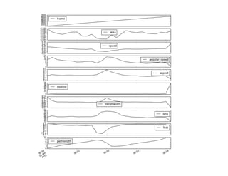
![In [11]: behav_resampled['angular_speed'].plot()
Out[11]: <matplotlib.axes._subplots.AxesSubplot at 0x10779b650>
time: 183 ms](https://image.slidesharecdn.com/usingthepythondatatoolkittimbersslides-150911211628-lva1-app6892/85/Using-the-python_data_toolkit_timbers_slides-22-320.jpg)
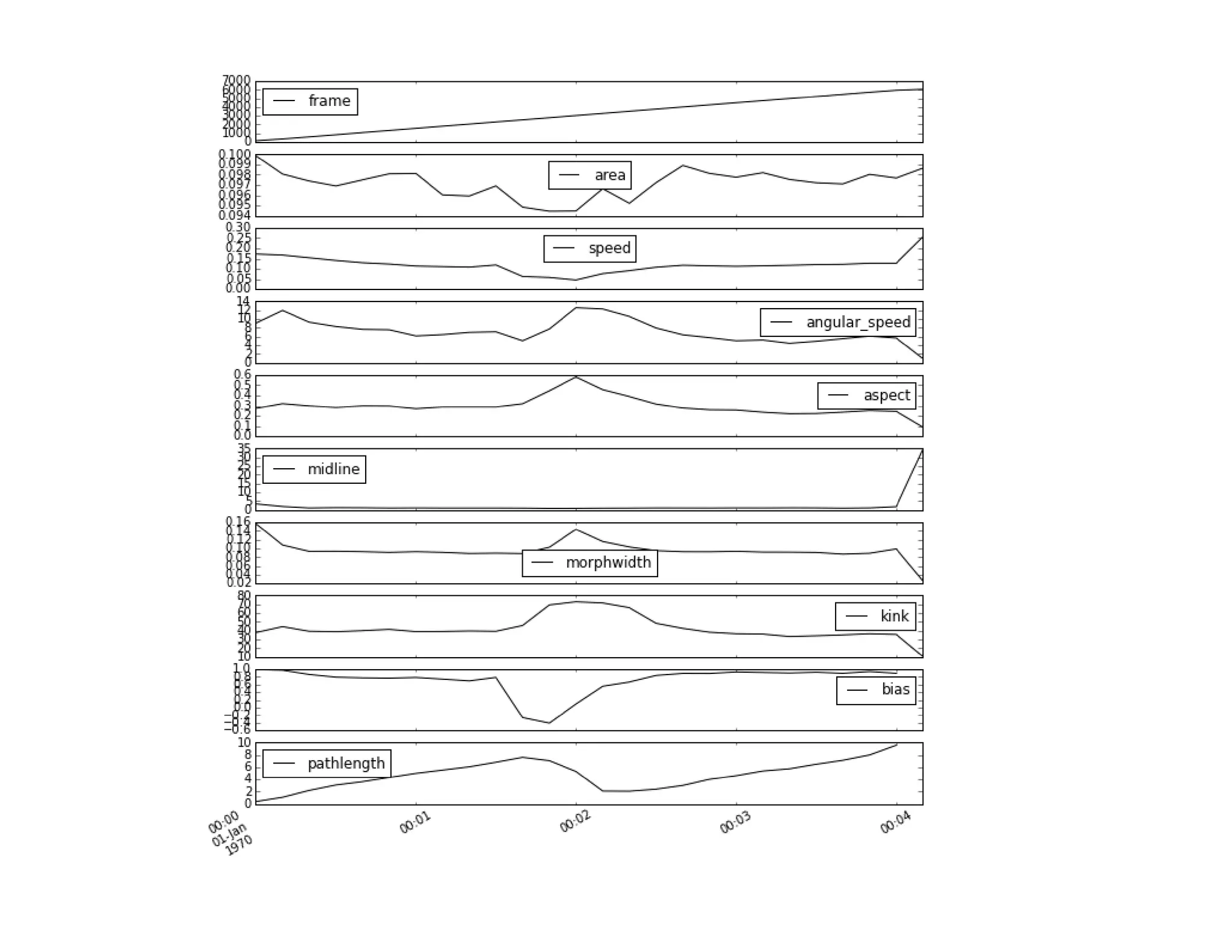
![In [12]: behav_resampled.plot(subplots=True, figsize = (10, 12))](https://image.slidesharecdn.com/usingthepythondatatoolkittimbersslides-150911211628-lva1-app6892/85/Using-the-python_data_toolkit_timbers_slides-23-320.jpg)
![Out[12]: array([<matplotlib.axes._subplots.AxesSubplot object at 0x112675890>,
<matplotlib.axes._subplots.AxesSubplot object at 0x10768a650>,
<matplotlib.axes._subplots.AxesSubplot object at 0x10770f150>,
<matplotlib.axes._subplots.AxesSubplot object at 0x108002610>,
<matplotlib.axes._subplots.AxesSubplot object at 0x109859790>,
<matplotlib.axes._subplots.AxesSubplot object at 0x108039610>,
<matplotlib.axes._subplots.AxesSubplot object at 0x10a16af10>,
<matplotlib.axes._subplots.AxesSubplot object at 0x10a1fc0d0>,
<matplotlib.axes._subplots.AxesSubplot object at 0x10a347e90>,
<matplotlib.axes._subplots.AxesSubplot object at 0x10ab0ce50>], dtype=object)](https://image.slidesharecdn.com/usingthepythondatatoolkittimbersslides-150911211628-lva1-app6892/85/Using-the-python_data_toolkit_timbers_slides-24-320.jpg)
![In [13]: behav_resampled[['speed', 'angular_speed', 'bias']].plot(subplots = True, figsize = (10,8))
time: 1.69 s
Out[13]: array([<matplotlib.axes._subplots.AxesSubplot object at 0x10bc4e250>,
<matplotlib.axes._subplots.AxesSubplot object at 0x10c981c50>,
<matplotlib.axes._subplots.AxesSubplot object at 0x10e7a1110>], dtype=object)
time: 541 ms](https://image.slidesharecdn.com/usingthepythondatatoolkittimbersslides-150911211628-lva1-app6892/85/Using-the-python_data_toolkit_timbers_slides-26-320.jpg)


![In [1]: ## load libraries
%matplotlib inline
import pandas as pd
import numpy as np
from pandas import set_option
set_option("display.max_rows", 4)
## magic to time cells in ipython notebook
%install_ext https://raw.github.com/cpcloud/ipython-autotime/master/autotime.py
%load_ext autotime
1. Loading data from a local text file
More details, see http://pandas.pydata.org/pandas-docs/stable/io.html (http://pandas.pydata.org/pandas-docs/stable/io.html)
Let's first load some behaviour data from a collection of wild-type worms.
Installed autotime.py. To use it, type:
%load_ext autotime](https://image.slidesharecdn.com/usingthepythondatatoolkittimbersslides-150911211628-lva1-app6892/75/Using-the-python_data_toolkit_timbers_slides-14-2048.jpg)
![In [2]: filename = 'data/behav.dat'
behav = pd.read_table(filename, sep = 's+')
behav
2. Dataframe data structures
For more details, see http://pandas.pydata.org/pandas-docs/stable/dsintro.html (http://pandas.pydata.org/pandas-docs/stable/dsintro.html)
Pandas provides access to data frame data structures. These tabular data objects allow you to mix and match arrays of different data types
in one "table".
Out[2]:
time: 642 ms
plate time strain frame area speed angular_speed aspect midline morphwidth kink
0 20141118_131037 5.065 N2 126 0.094770 0.3600 0.8706 0.0822 12.1000 1.0000 0.000
1 20141118_131037 5.109 N2 127 0.094770 0.3600 0.8630 0.0819 5.9000 1.0000 0.007
... ... ... ... ... ... ... ... ... ... ... ...
249997 20141118_132717 249.048 N2 6158 0.108621 0.0792 0.5000 0.1470 0.9943 0.0906 41.200
249998 20141118_132717 249.093 N2 6159 0.107892 0.0693 0.6000 0.1520 1.0019 0.0903 42.900
249999 rows × 13 columns](https://image.slidesharecdn.com/usingthepythondatatoolkittimbersslides-150911211628-lva1-app6892/75/Using-the-python_data_toolkit_timbers_slides-15-2048.jpg)
![In [3]: print behav.dtypes
3. Element-wise mathematics
Suppose we want to add a new column that is a combination of two columns in our dataset. Similar to numpy, Pandas lets us do this easily
and deals with doing math between columns on an element by element basis. For example, We are interested in the ratio of the midline
length divided by the morphwidth to look at whether worms are crawling in a straight line or curling back on themselves (e.g., during a turn).
In [4]: ## vectorization takes 49.3 ms
behav['mid_width_ratio'] = behav['morphwidth']/behav['midline']
behav[['morphwidth', 'midline', 'mid_width_ratio']].head()
plate object
time float64
...
bias float64
pathlength float64
dtype: object
time: 4.85 ms
Out[4]: morphwidth midline mid_width_ratio
0 1 12.1 0.082645
1 1 5.9 0.169492
... ... ... ...
3 1 14.9 0.067114
4 1 6.3 0.158730
5 rows × 3 columns
time: 57.6 ms](https://image.slidesharecdn.com/usingthepythondatatoolkittimbersslides-150911211628-lva1-app6892/75/Using-the-python_data_toolkit_timbers_slides-16-2048.jpg)
![In [ ]: ## looping takes 1 min 44s
mid_width_ratio = np.empty(len(behav['morphwidth']), dtype='float64')
for i in range(1,len(behav['morphwidth'])):
mid_width_ratio[i] =+ behav.loc[i,'morphwidth']/behav.loc[i,'midline']
behav['mid_width_ratio'] = mid_width_ratio
behav[['morphwidth', 'midline', 'mid_width_ratio']].head()
apply()
For more details, see: http://pandas.pydata.org/pandas-docs/stable/generated/pandas.DataFrame.apply.html
(http://pandas.pydata.org/pandas-docs/stable/generated/pandas.DataFrame.apply.html)
Another bonus about using Pandas is the apply function - this allows you to apply any function to a select column(s) or row(s) of a
dataframe, or accross the entire dataframe.
In [5]: ## custom function to center data
def center(data):
return data - data.mean()
time: 1.49 ms](https://image.slidesharecdn.com/usingthepythondatatoolkittimbersslides-150911211628-lva1-app6892/75/Using-the-python_data_toolkit_timbers_slides-17-2048.jpg)
![In [6]: ## center all data on a column basis
behav.iloc[:,4:].apply(center).head()
4. Working with time series data
Indices
For more details, see http://pandas.pydata.org/pandas-docs/stable/indexing.html (http://pandas.pydata.org/pandas-
docs/stable/indexing.html)
Given that this is time series data we will want to set the index to time, we can do this while we read in the data.
Out[6]:
time: 55.3 ms
area speed angular_speed aspect midline morphwidth kink bias pathlength mid_width_ratio
0 -0.002280 0.249039 -6.313001 -0.219804 11.004384 0.904059 -43.962917 NaN NaN -0.029877
1 -0.002280 0.249039 -6.320601 -0.220104 4.804384 0.904059 -43.955917 NaN NaN 0.056970
... ... ... ... ... ... ... ... ... ... ...
3 -0.000093 0.229039 -6.279701 -0.220304 13.804384 0.904059 -43.942917 NaN NaN -0.045408
4 0.000636 0.221039 -6.257501 -0.217504 5.204384 0.904059 -43.935917 NaN NaN 0.046208
5 rows × 10 columns](https://image.slidesharecdn.com/usingthepythondatatoolkittimbersslides-150911211628-lva1-app6892/75/Using-the-python_data_toolkit_timbers_slides-18-2048.jpg)
![In [7]: behav = pd.read_table(filename, sep = 's+', index_col='time')
behav
To utilize functions built into Pandas to deal with time series data, let's convert our time to a date time object using the to_datetime()
function.
In [8]: behav.index.dtype
Out[7]:
time: 609 ms
plate strain frame area speed angular_speed aspect midline morphwidth kink bias
time
5.065 20141118_131037 N2 126 0.094770 0.3600 0.8706 0.0822 12.1000 1.0000 0.000 NaN
5.109 20141118_131037 N2 127 0.094770 0.3600 0.8630 0.0819 5.9000 1.0000 0.007 NaN
... ... ... ... ... ... ... ... ... ... ... ...
249.048 20141118_132717 N2 6158 0.108621 0.0792 0.5000 0.1470 0.9943 0.0906 41.200 1
249.093 20141118_132717 N2 6159 0.107892 0.0693 0.6000 0.1520 1.0019 0.0903 42.900 1
249999 rows × 12 columns
Out[8]: dtype('float64')
time: 2.53 ms](https://image.slidesharecdn.com/usingthepythondatatoolkittimbersslides-150911211628-lva1-app6892/75/Using-the-python_data_toolkit_timbers_slides-19-2048.jpg)
![In [9]: behav.index = pd.to_datetime(behav.index, unit='s')
print behav.index.dtype
behav
Now that our index is of datetime object, we can use the resample function to get time intervals. With this function you can choose the time
interval as well as how to downsample (mean, sum, etc.)
datetime64[ns]
Out[9]:
time: 394 ms
plate strain frame area speed angular_speed aspect midline morphwidth kink
1970-01-01
00:00:05.065
20141118_131037 N2 126 0.094770 0.3600 0.8706 0.0822 12.1000 1.0000 0.000
1970-01-01
00:00:05.109
20141118_131037 N2 127 0.094770 0.3600 0.8630 0.0819 5.9000 1.0000 0.007
... ... ... ... ... ... ... ... ... ... ...
1970-01-01
00:04:09.048
20141118_132717 N2 6158 0.108621 0.0792 0.5000 0.1470 0.9943 0.0906 41.200
1970-01-01
00:04:09.093
20141118_132717 N2 6159 0.107892 0.0693 0.6000 0.1520 1.0019 0.0903 42.900
249999 rows × 12 columns](https://image.slidesharecdn.com/usingthepythondatatoolkittimbersslides-150911211628-lva1-app6892/75/Using-the-python_data_toolkit_timbers_slides-20-2048.jpg)
![In [10]: behav_resampled = behav.resample('10s', how=('mean'))
behav_resampled
5. Quick and easy visualization
For more details, see: http://pandas.pydata.org/pandas-docs/version/0.15.0/visualization.html (http://pandas.pydata.org/pandas-
docs/version/0.15.0/visualization.html)
Out[10]:
time: 103 ms
frame area speed angular_speed aspect midline morphwidth kink bias pathlength
1970-
01-01
00:00:00
158.970096 0.099870 0.172162 9.021929 0.271491 3.385725 0.156643 37.793984 0.987238 0.379338
1970-
01-01
00:00:10
362.347271 0.098067 0.166863 11.942732 0.319444 1.880583 0.107296 44.520299 0.969474 1.080874
... ... ... ... ... ... ... ... ... ... ...
1970-
01-01
00:04:00
5924.536608 0.097678 0.127150 5.646088 0.242850 1.785435 0.098452 35.647127 0.889103 9.590879
1970-
01-01
00:04:10
6041.902439 0.098643 0.255963 0.910815 0.088282 34.607500 0.025641 10.396449 NaN NaN
26 rows × 10 columns](https://image.slidesharecdn.com/usingthepythondatatoolkittimbersslides-150911211628-lva1-app6892/75/Using-the-python_data_toolkit_timbers_slides-21-2048.jpg)
![In [11]: behav_resampled['angular_speed'].plot()
Out[11]: <matplotlib.axes._subplots.AxesSubplot at 0x10779b650>
time: 183 ms](https://image.slidesharecdn.com/usingthepythondatatoolkittimbersslides-150911211628-lva1-app6892/75/Using-the-python_data_toolkit_timbers_slides-22-2048.jpg)
![In [12]: behav_resampled.plot(subplots=True, figsize = (10, 12))](https://image.slidesharecdn.com/usingthepythondatatoolkittimbersslides-150911211628-lva1-app6892/75/Using-the-python_data_toolkit_timbers_slides-23-2048.jpg)
![Out[12]: array([<matplotlib.axes._subplots.AxesSubplot object at 0x112675890>,
<matplotlib.axes._subplots.AxesSubplot object at 0x10768a650>,
<matplotlib.axes._subplots.AxesSubplot object at 0x10770f150>,
<matplotlib.axes._subplots.AxesSubplot object at 0x108002610>,
<matplotlib.axes._subplots.AxesSubplot object at 0x109859790>,
<matplotlib.axes._subplots.AxesSubplot object at 0x108039610>,
<matplotlib.axes._subplots.AxesSubplot object at 0x10a16af10>,
<matplotlib.axes._subplots.AxesSubplot object at 0x10a1fc0d0>,
<matplotlib.axes._subplots.AxesSubplot object at 0x10a347e90>,
<matplotlib.axes._subplots.AxesSubplot object at 0x10ab0ce50>], dtype=object)](https://image.slidesharecdn.com/usingthepythondatatoolkittimbersslides-150911211628-lva1-app6892/75/Using-the-python_data_toolkit_timbers_slides-24-2048.jpg)
![In [13]: behav_resampled[['speed', 'angular_speed', 'bias']].plot(subplots = True, figsize = (10,8))
time: 1.69 s
Out[13]: array([<matplotlib.axes._subplots.AxesSubplot object at 0x10bc4e250>,
<matplotlib.axes._subplots.AxesSubplot object at 0x10c981c50>,
<matplotlib.axes._subplots.AxesSubplot object at 0x10e7a1110>], dtype=object)
time: 541 ms](https://image.slidesharecdn.com/usingthepythondatatoolkittimbersslides-150911211628-lva1-app6892/75/Using-the-python_data_toolkit_timbers_slides-26-2048.jpg)

This document discusses using the Pandas Python data analysis library. It describes how Pandas makes it easy to load, manipulate, and visualize complex tabular data. Specific features highlighted include loading data from files, creating and manipulating dataframe data structures, performing element-wise math operations on columns, working with time series data through indexing and resampling, and quick visualization of data.


