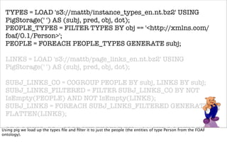
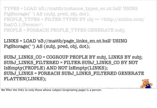
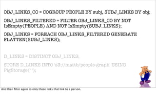
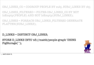
Download as PDF, PPTX


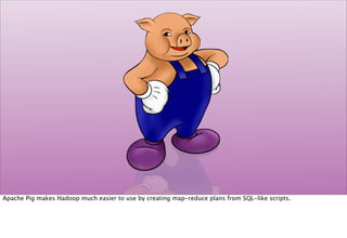


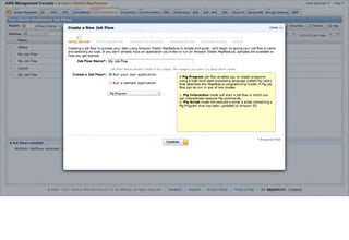
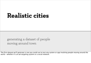
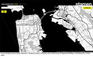
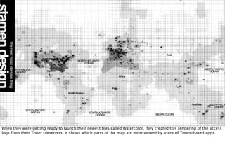
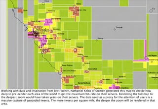

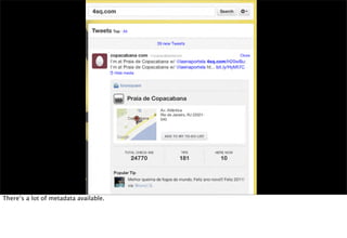
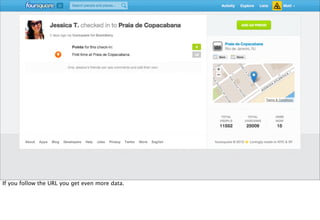
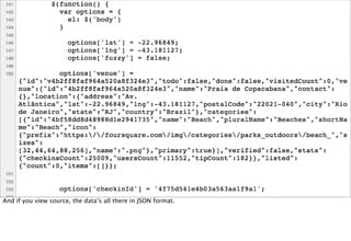


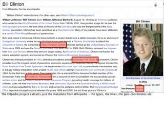
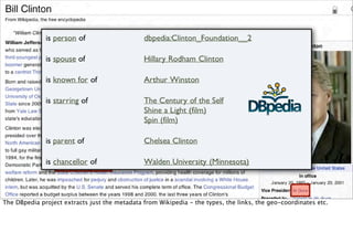
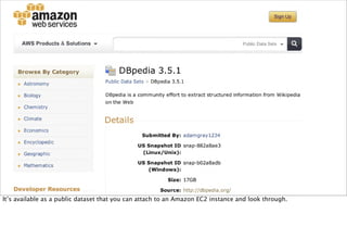
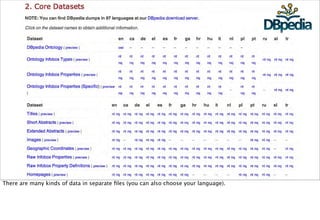
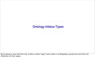
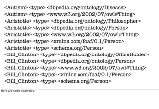

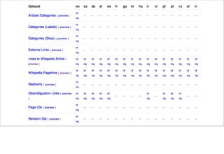


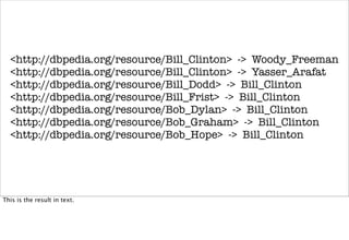
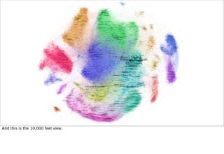


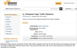
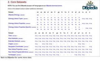
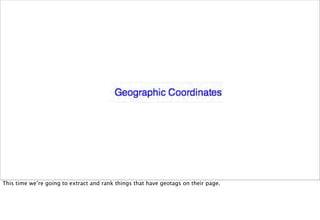
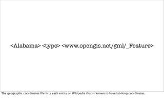
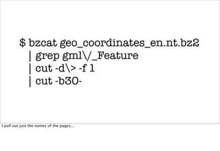
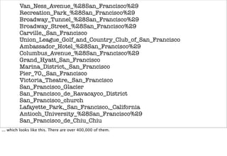
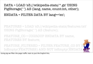

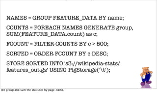


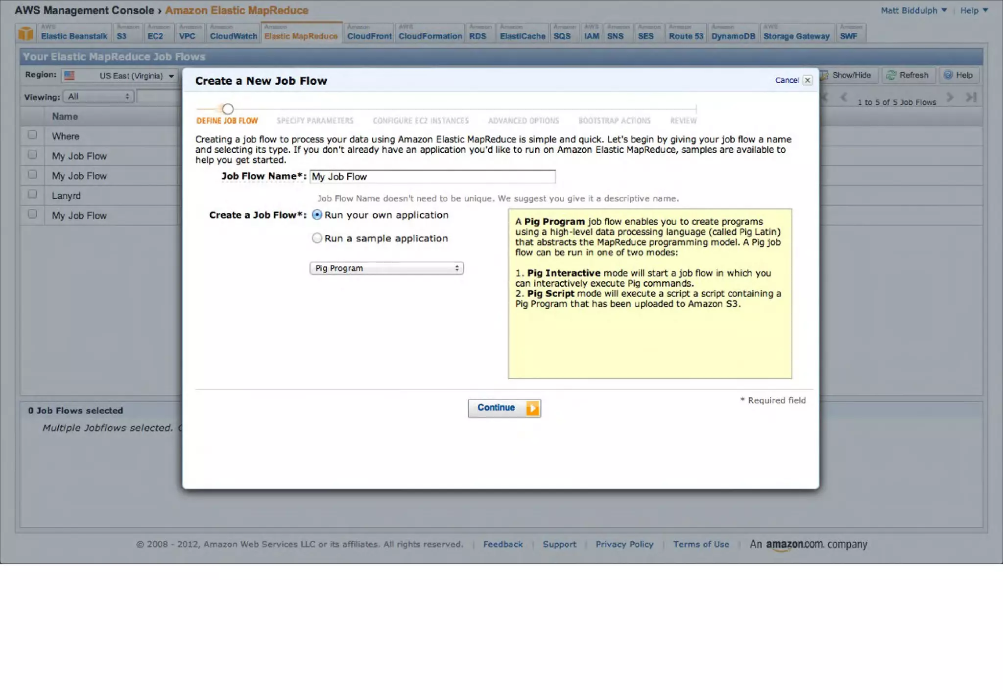

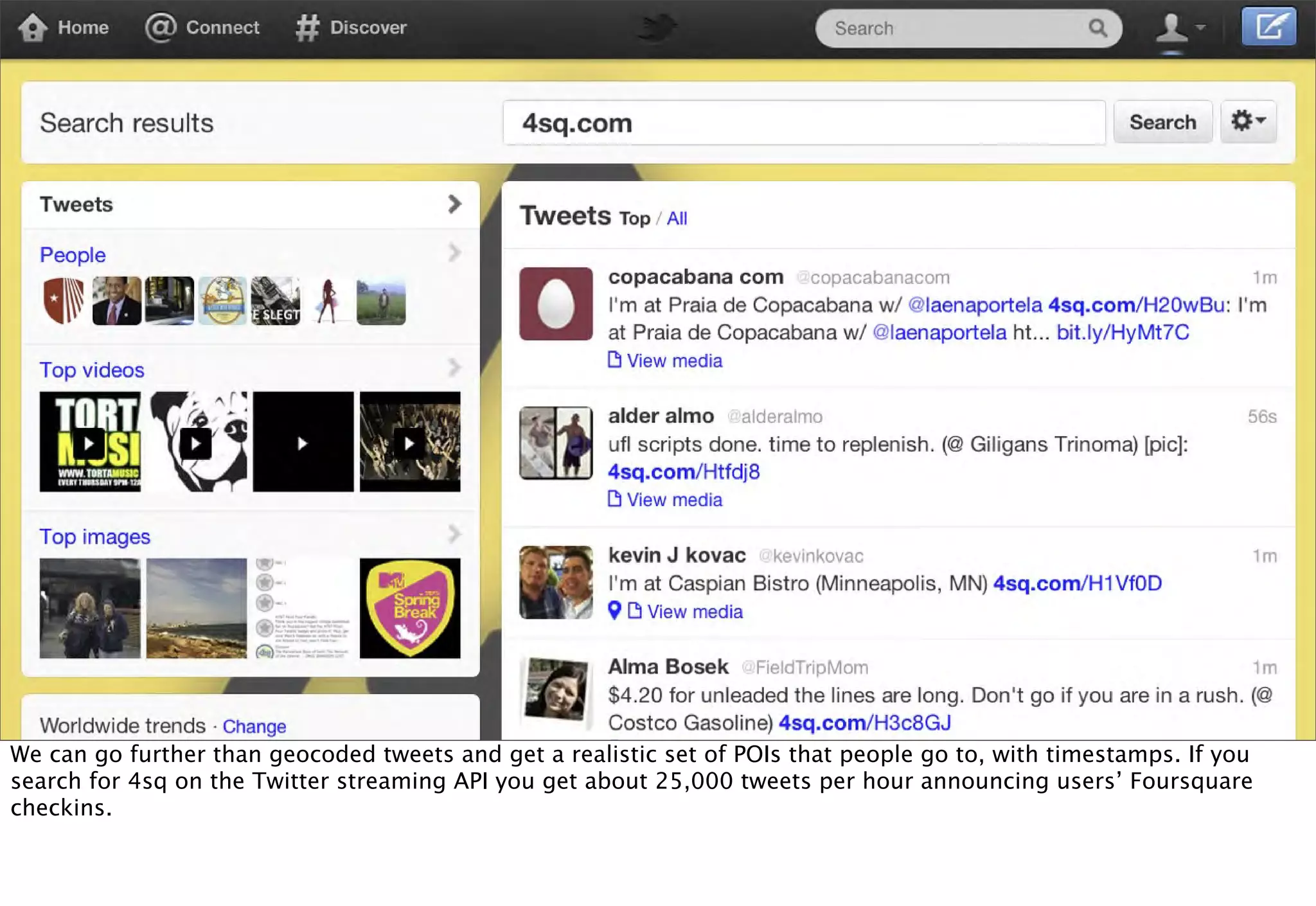

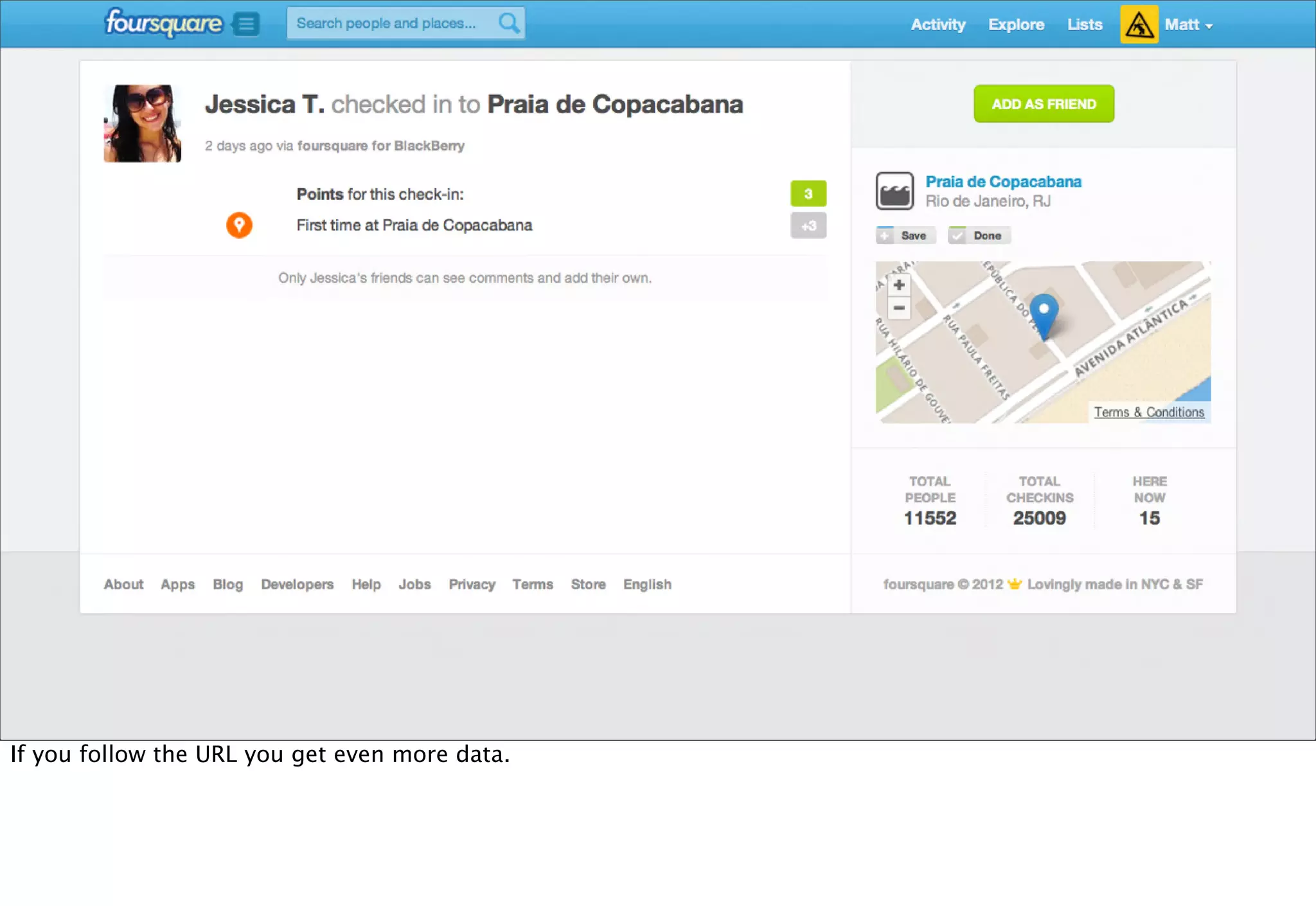
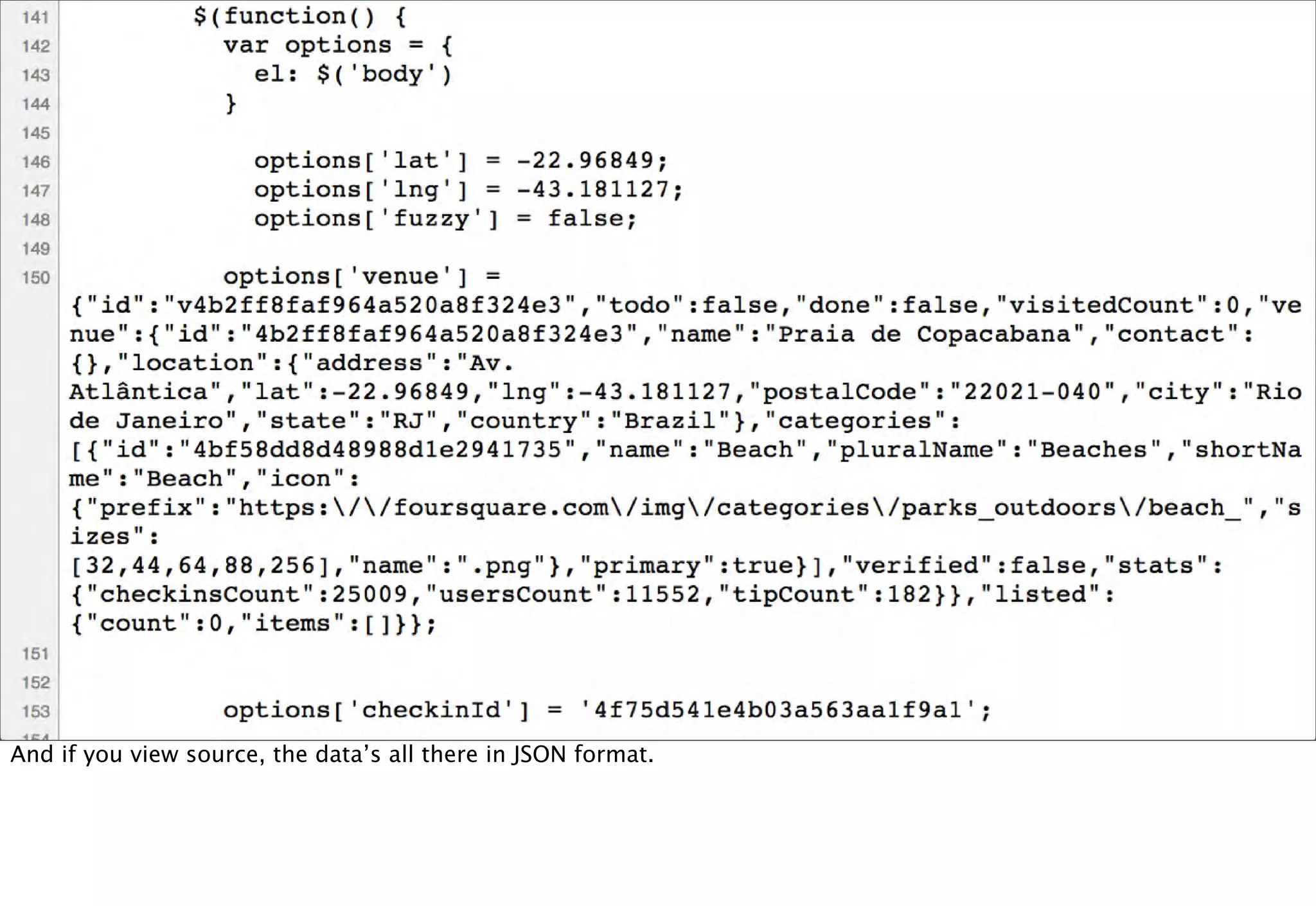

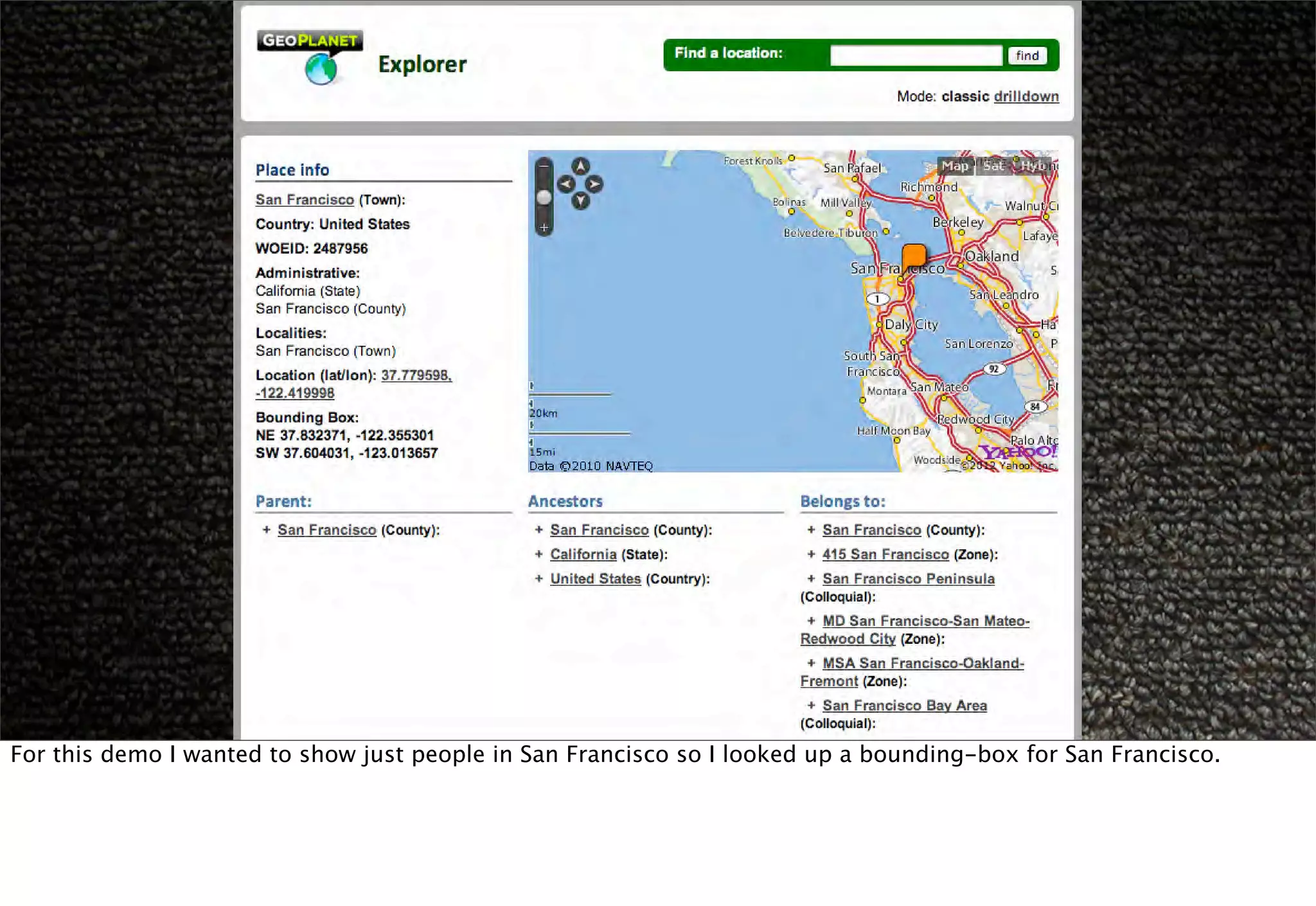
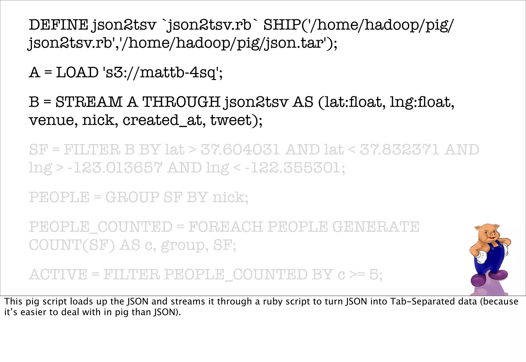
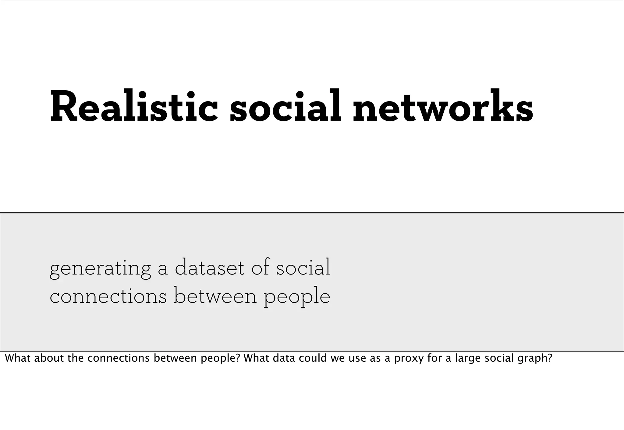

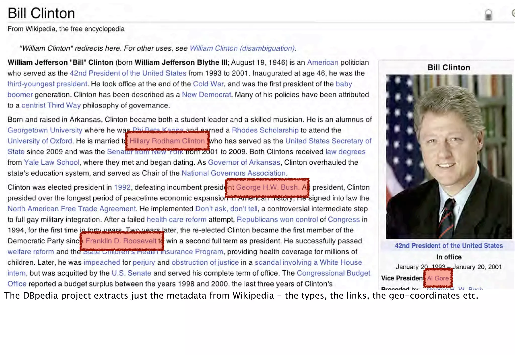

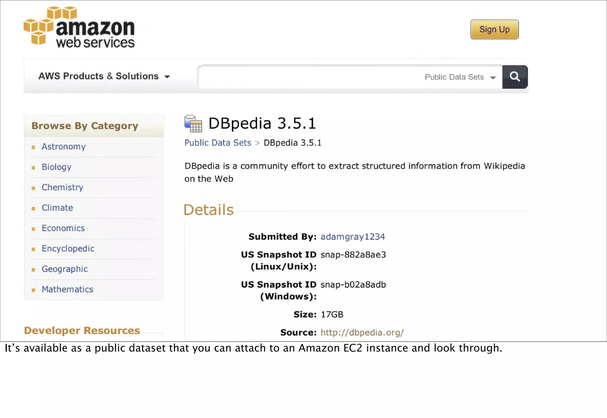
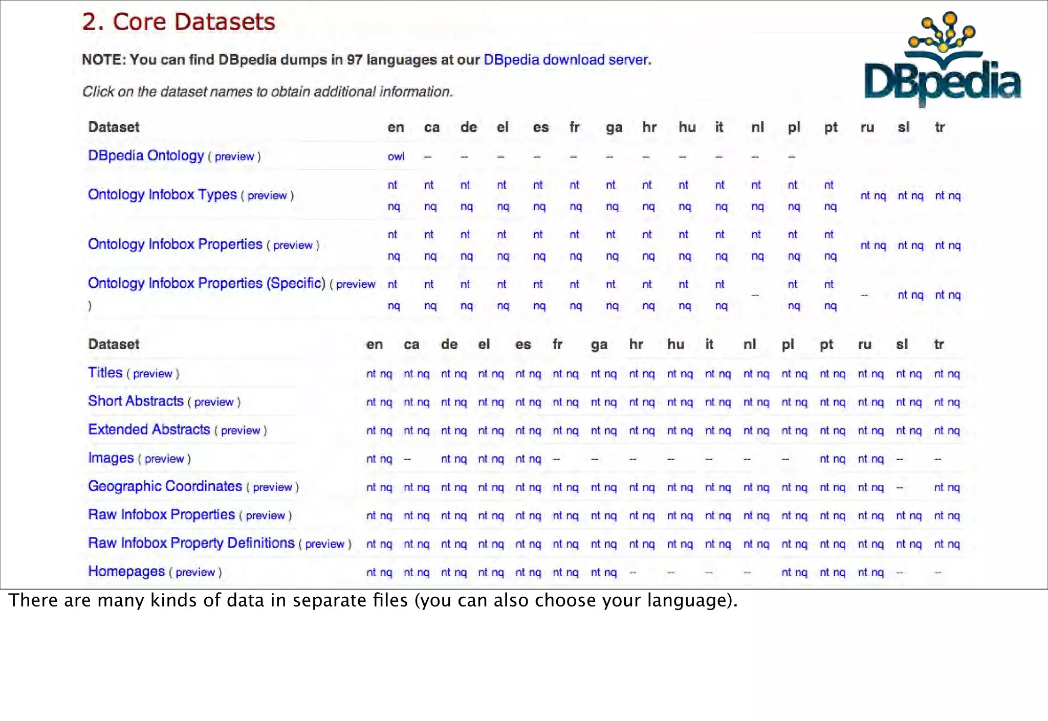
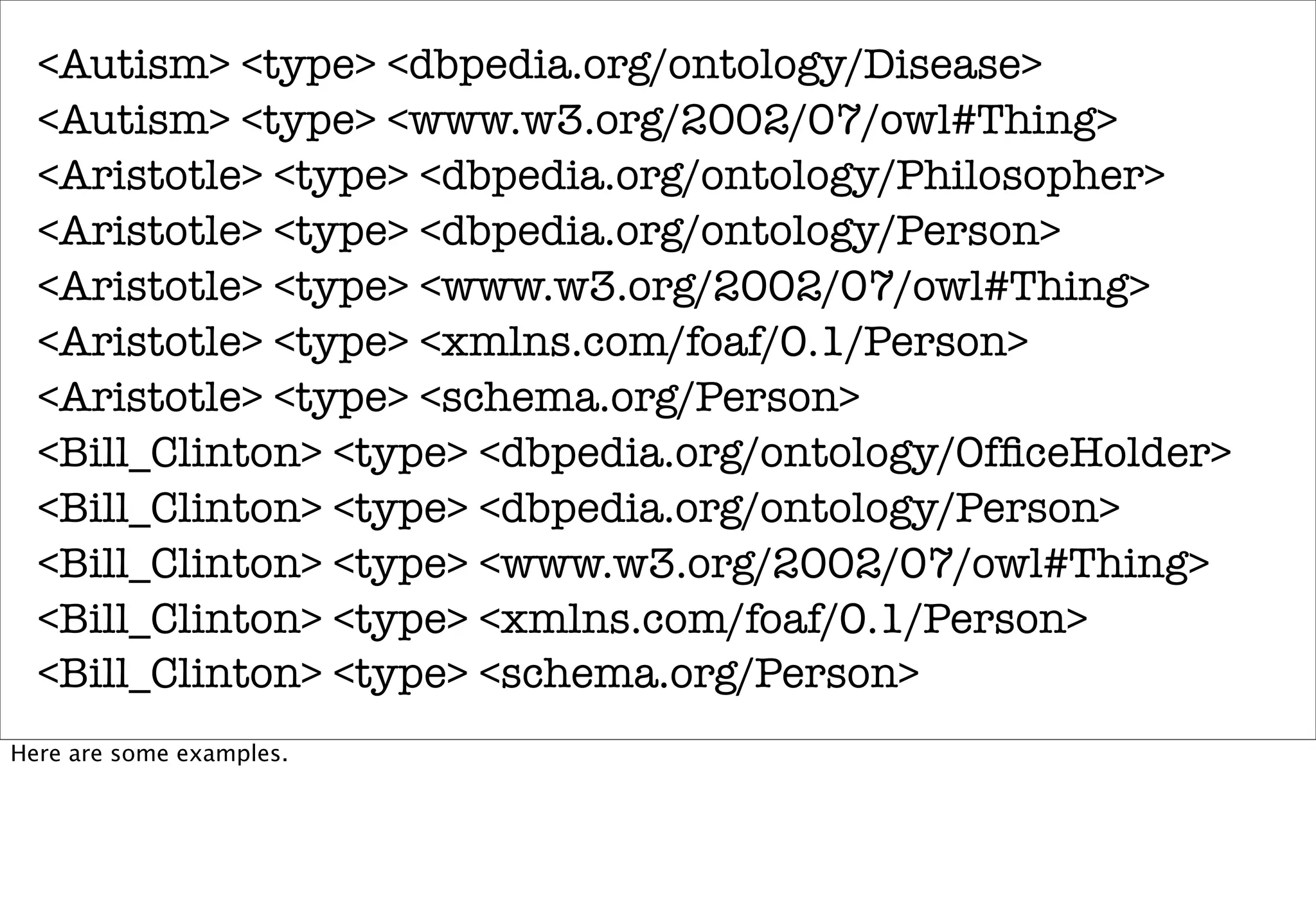
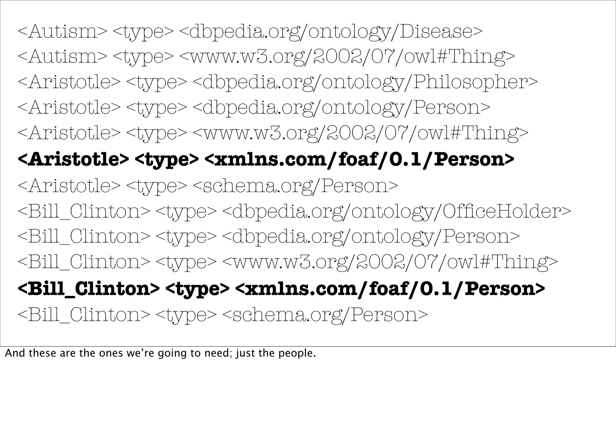

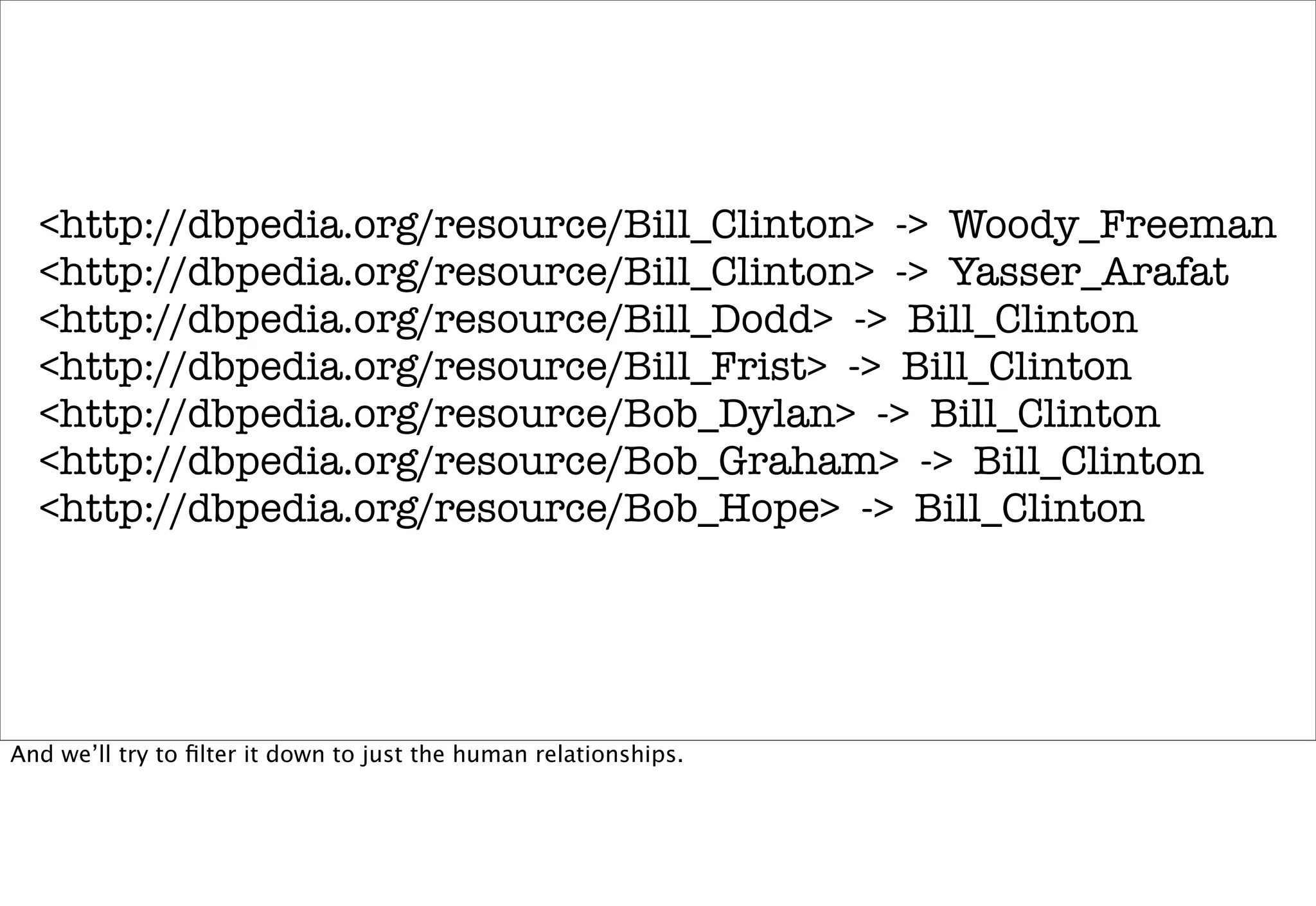
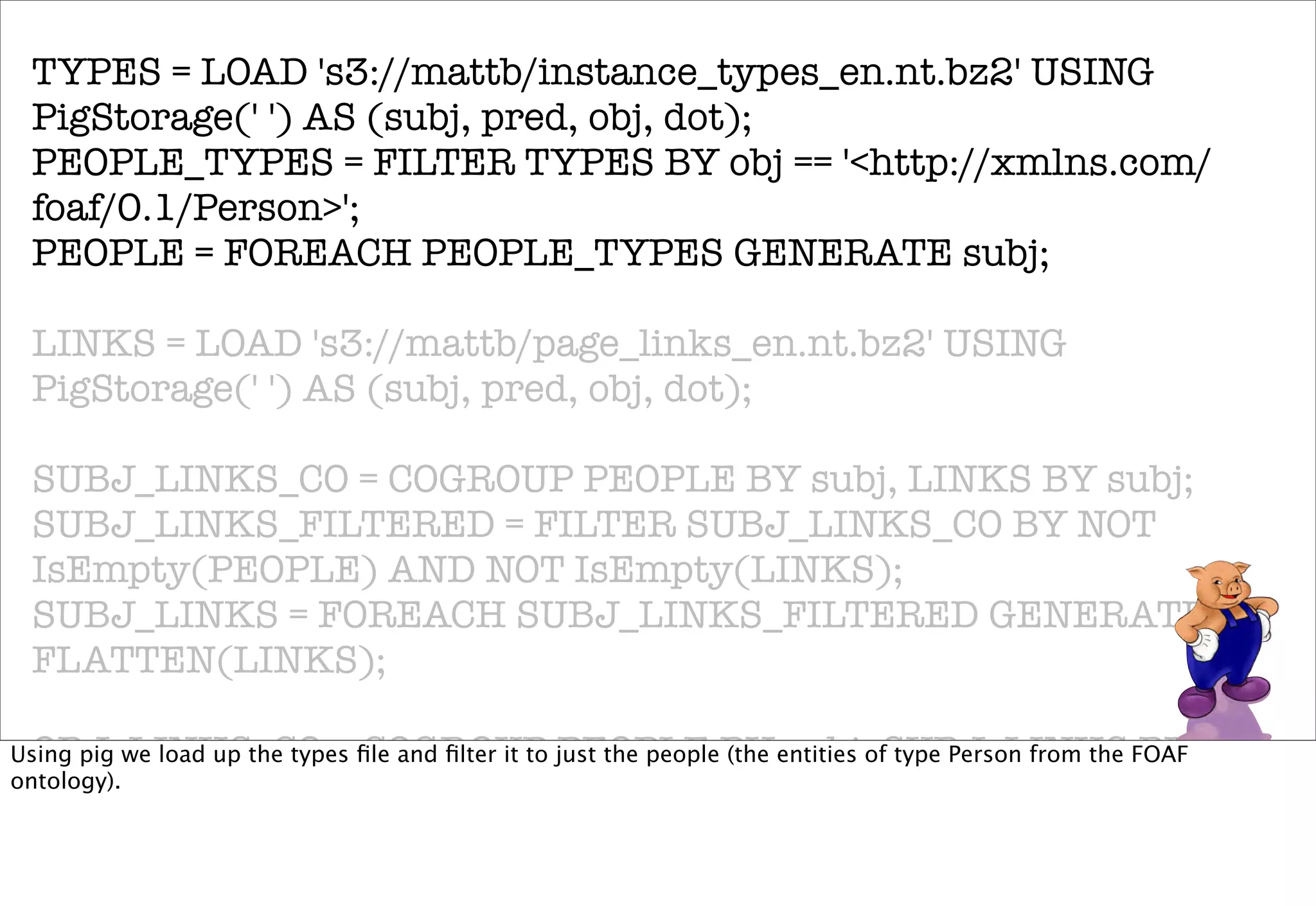
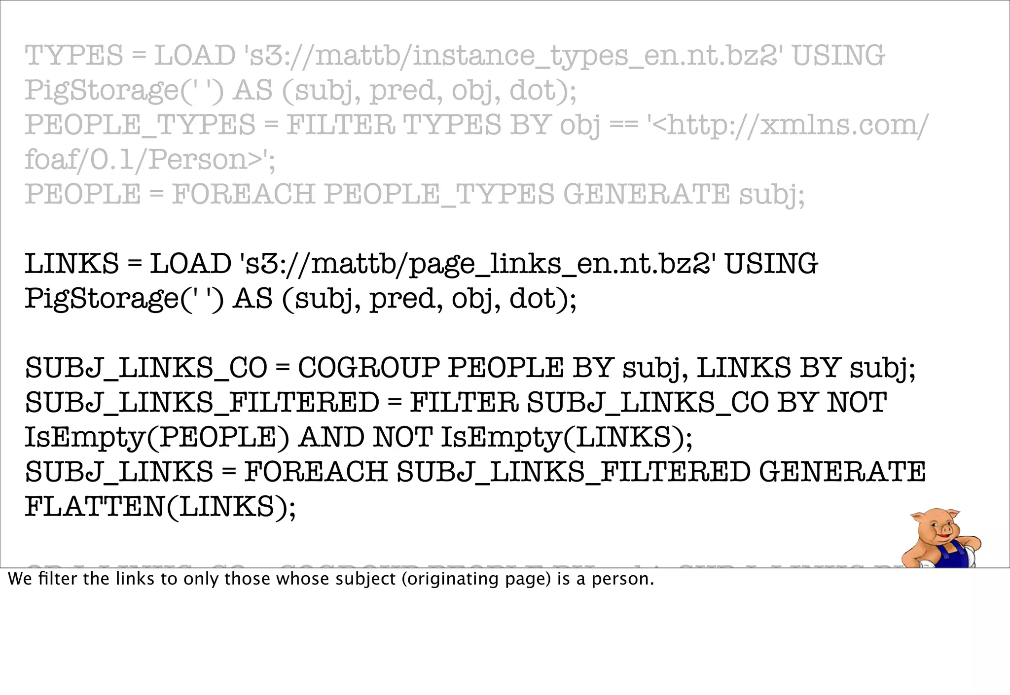


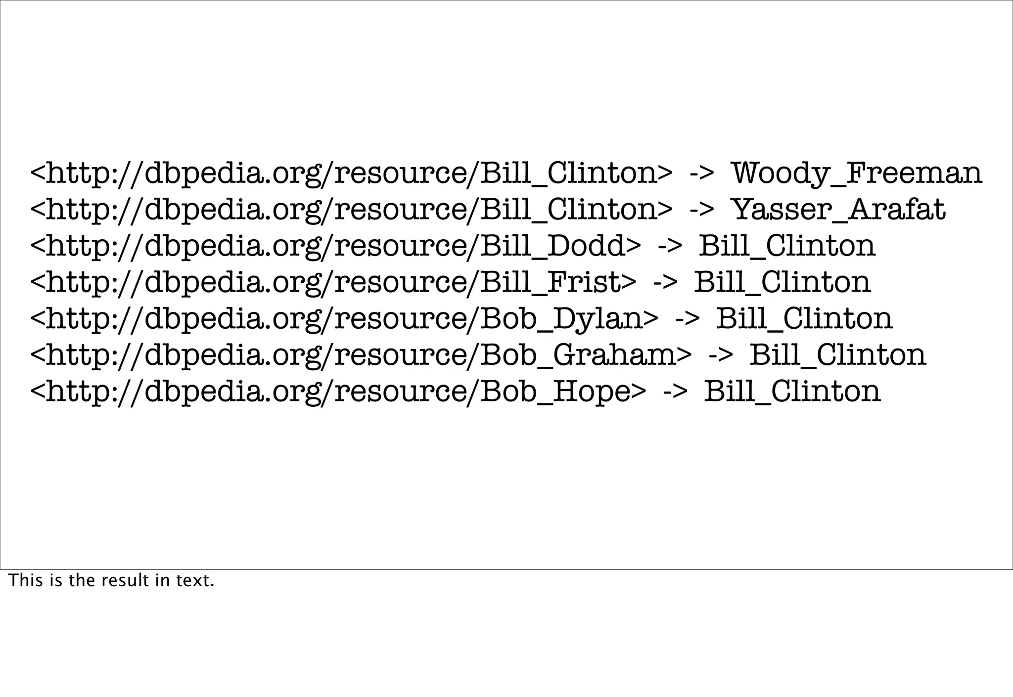
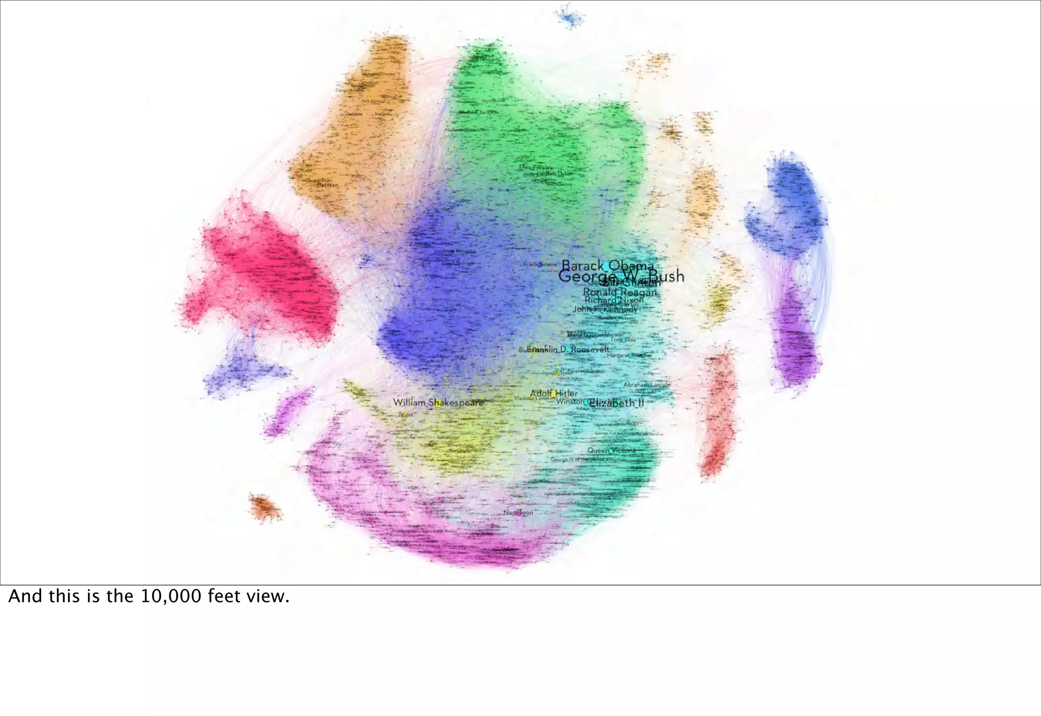
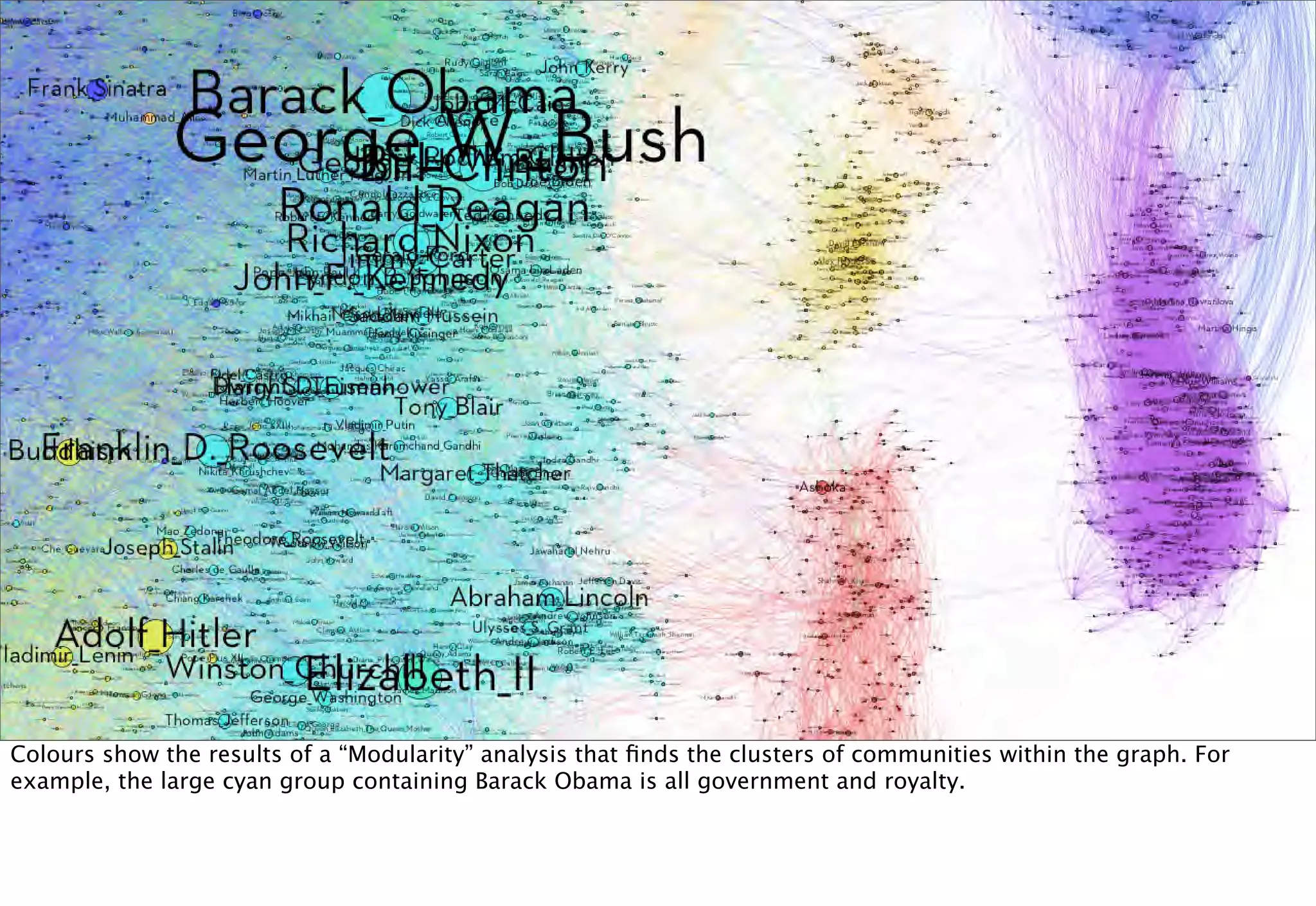


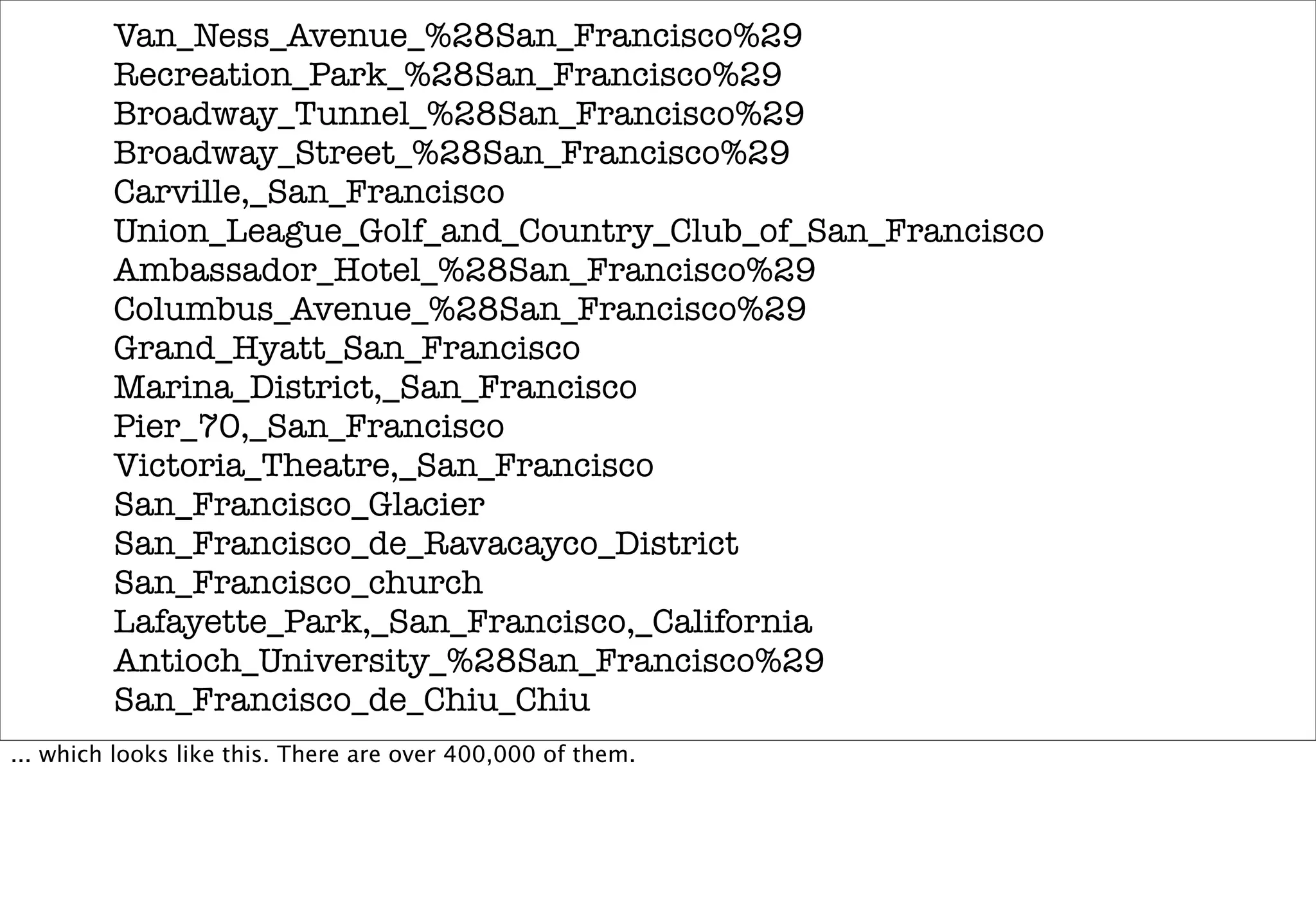

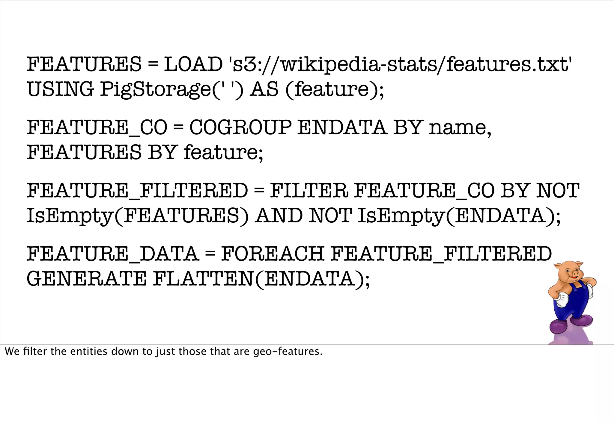
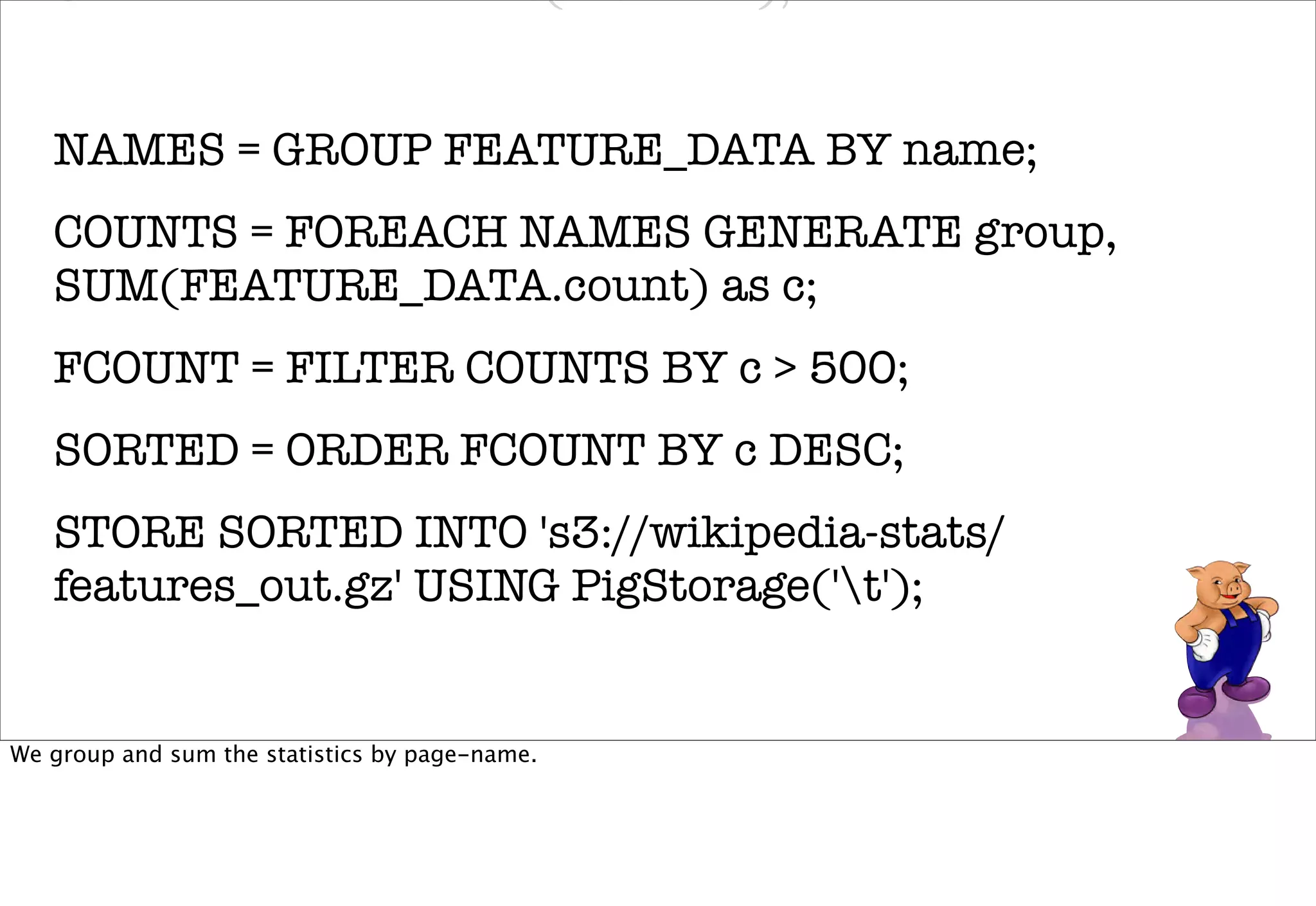
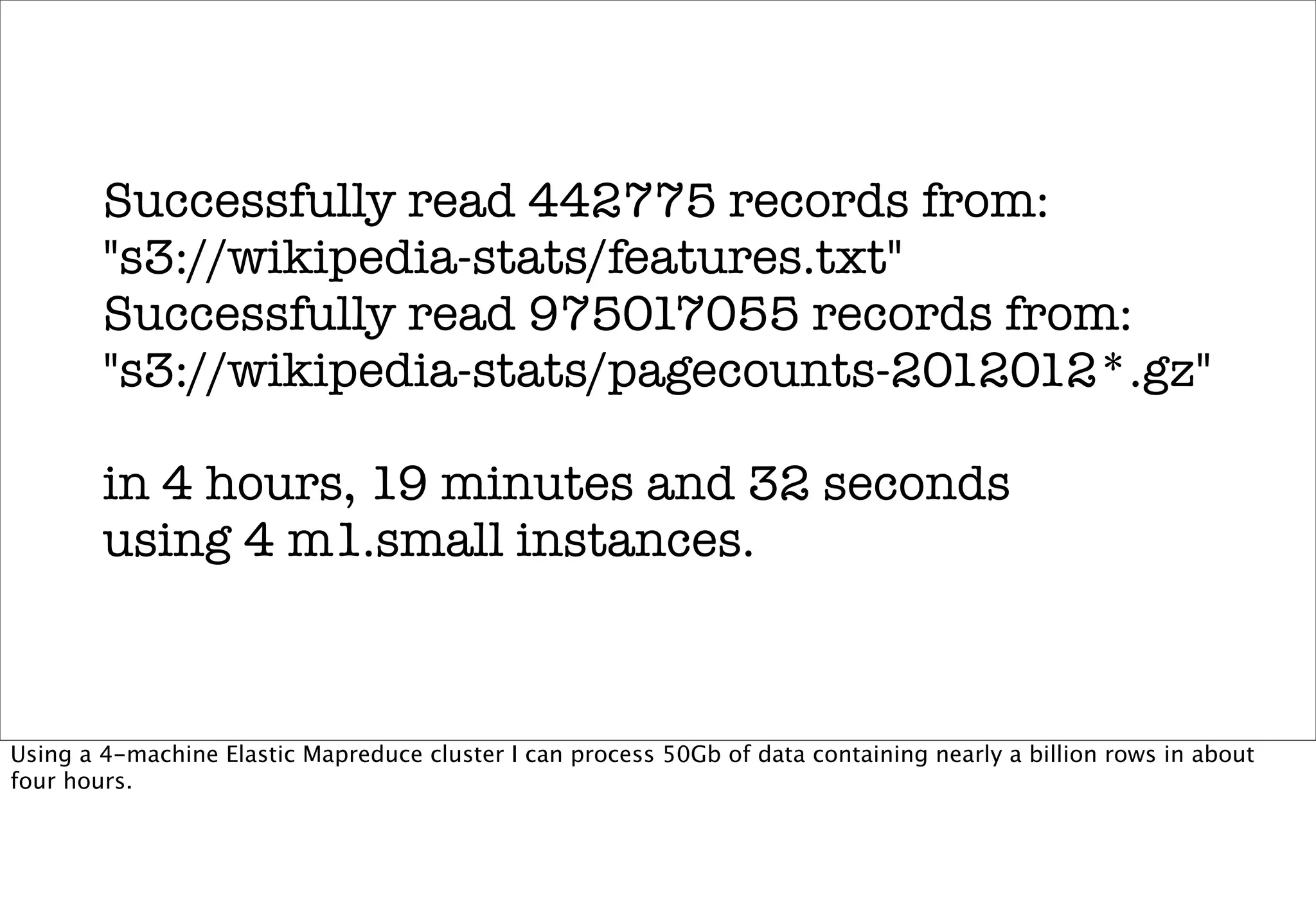


The document discusses prototyping location apps with real data. It describes generating realistic datasets of people moving around cities by gathering check-in data from Foursquare tweets and visualizing the check-ins on maps. It also discusses generating social networks by extracting people and connection data from Wikipedia and DBpedia, including types of entities and links between pages. Code examples are provided to load and filter this data using Pig scripts on Amazon EMR.


![UiPath Automation Suite Installation (Hands-On) [2/3]](https://cdn.slidesharecdn.com/ss_thumbnails/automationsuitecommunitysession2-251015095633-a6d862f1-thumbnail.jpg?width=600ounds&width=560&fit=bounds)


