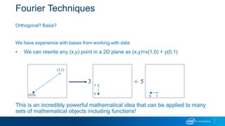
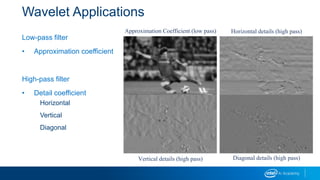
The document discusses various techniques for edge detection and line detection in images, including:
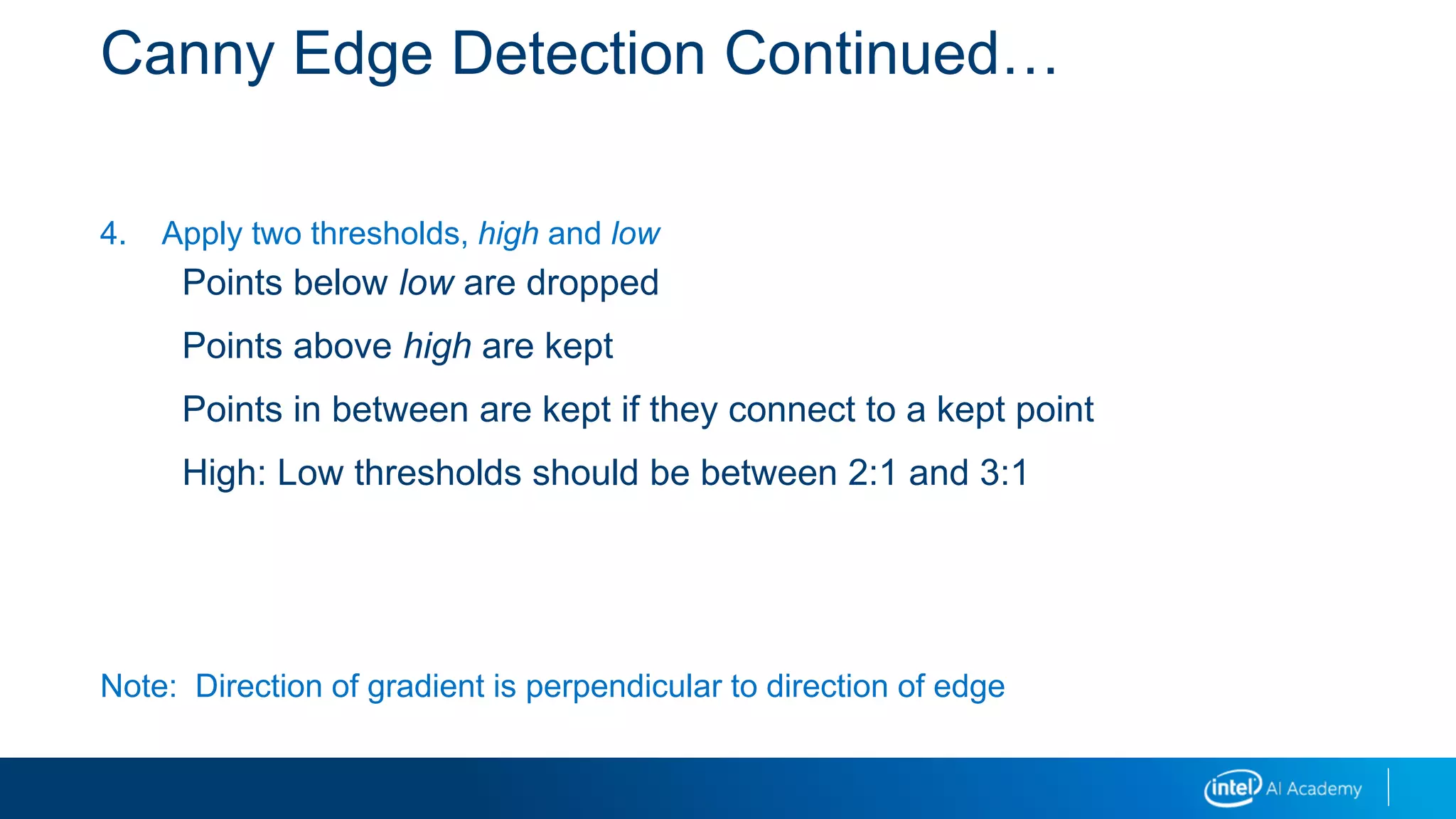
- Canny edge detection, which uses thresholds to detect and link edges.
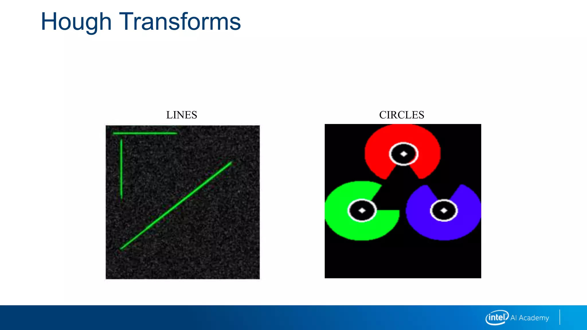
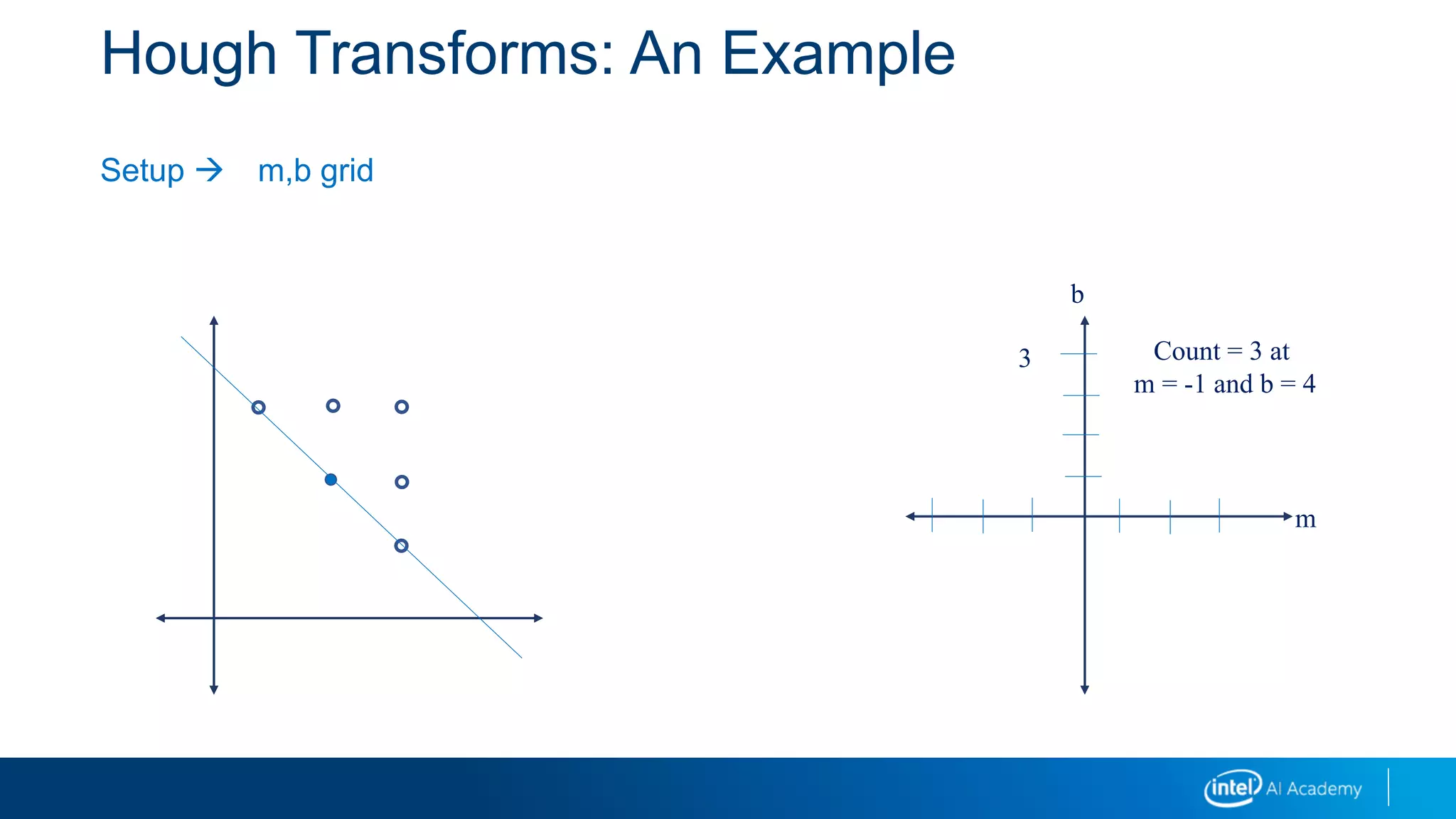
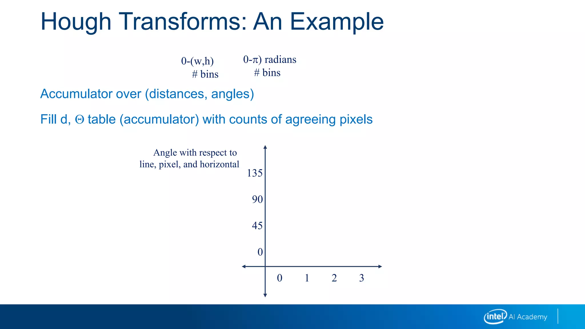
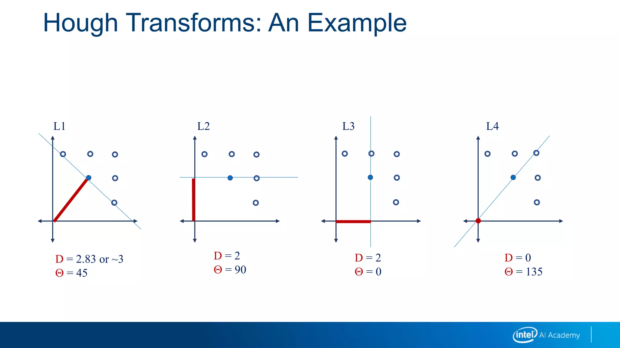
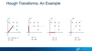
- Hough transforms, which detect shapes like lines and circles by counting points that agree with a shape model.
- RANSAC for line detection, which forms line hypotheses from random samples and counts supporting points.
- Techniques for thinning thick edges and detecting edge contours.


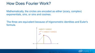

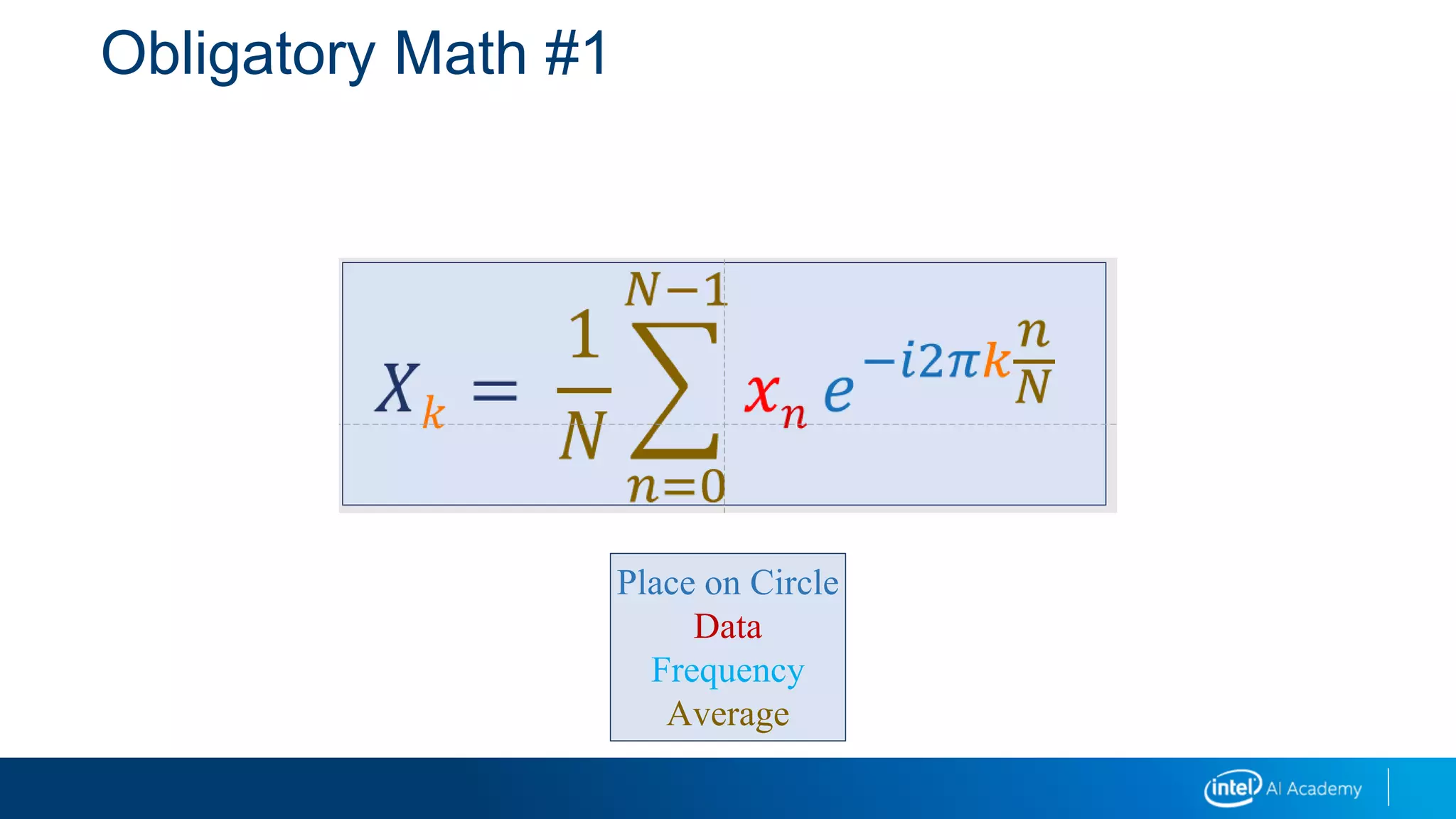
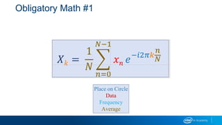
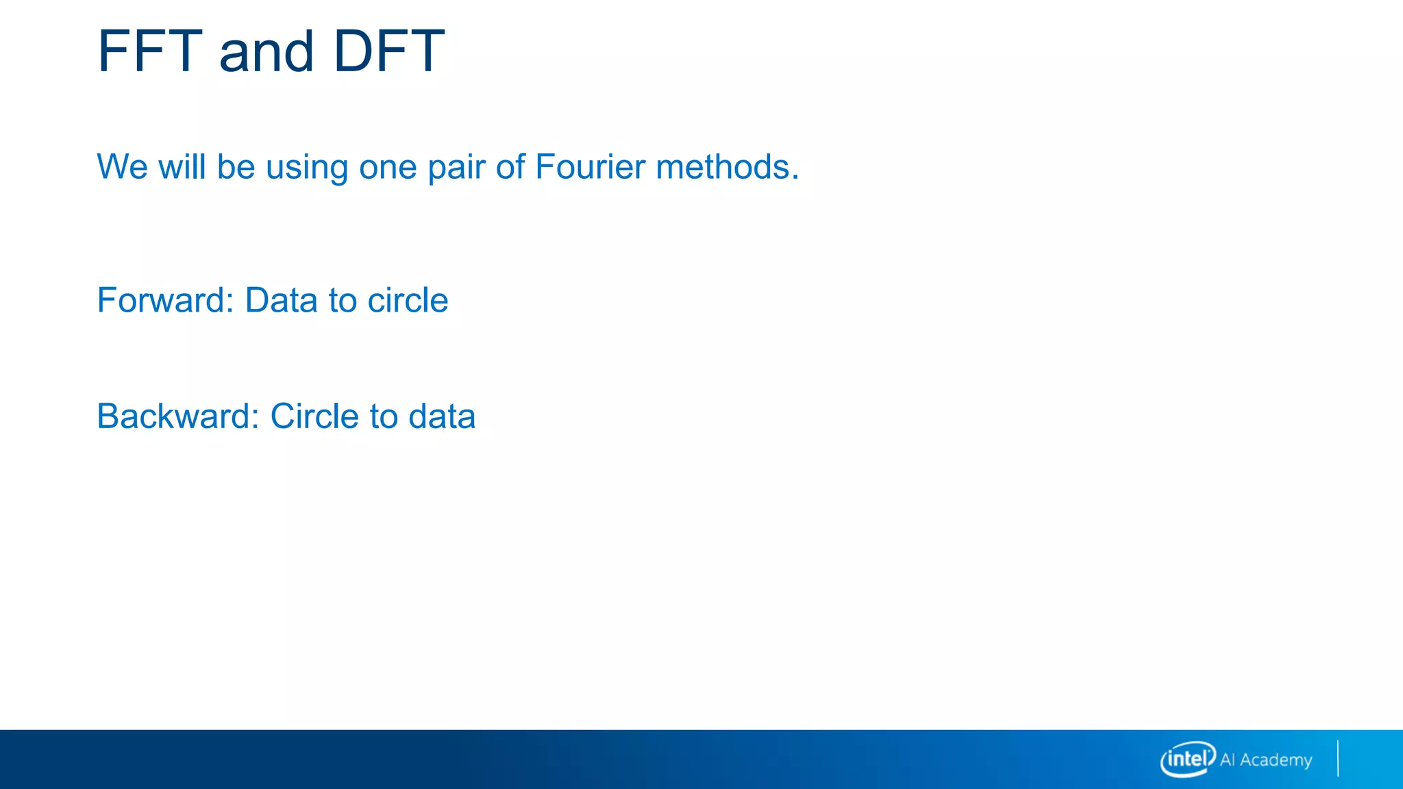
![FFT and DFT: Forward
Forward: Data to circle
Input fdata([0,N-1]])
Output fcircles([0,N-1])
The input function tells us our data values
Input has N data values
Output has N circles
The output function tells us characteristics of the circles in our rewrites](https://image.slidesharecdn.com/04imagetransformationsii-190218095700/85/04-image-transformations_ii-19-320.jpg)
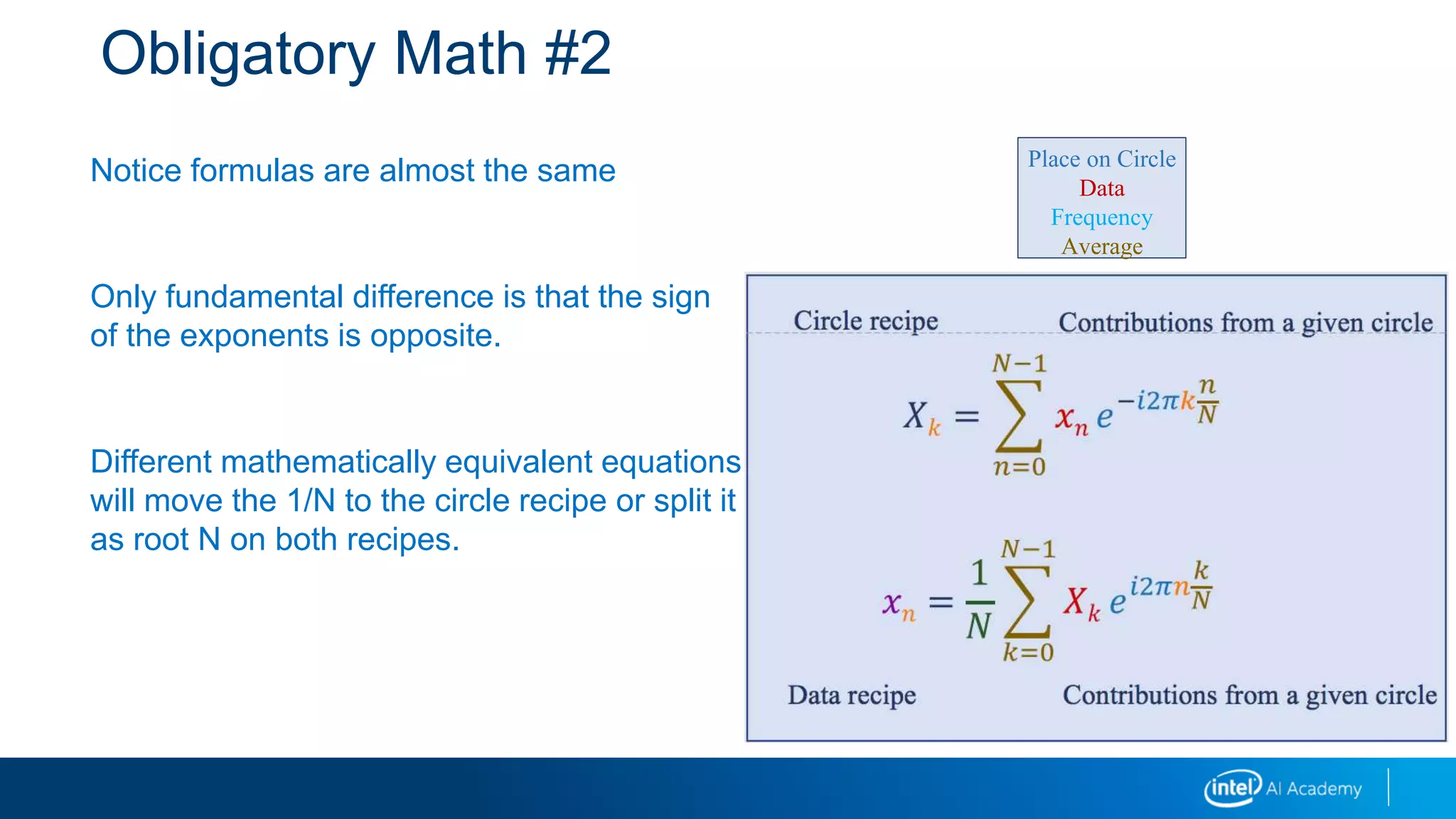
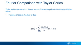
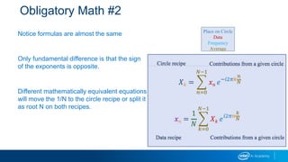
![FFT and DFT: Backward
Backward: Circle to data
Input fcircles([0,N-1]])
Output fdata([0,N-1])
Here we are going from an input function in terms of circles to an output
function in terms of our data
Input has N circles
Output has N data values](https://image.slidesharecdn.com/04imagetransformationsii-190218095700/85/04-image-transformations_ii-20-320.jpg)
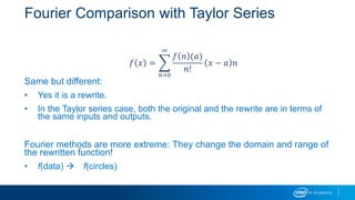
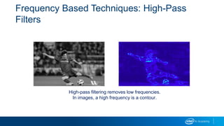
![FFT and DFT: p
You might be worried that neither of these are necessarily functions of, or around, a
circle.
What is a function of a circle?
• A function of a circle is defined for each angle of a walk around a circle [0, 2p]
radians](https://image.slidesharecdn.com/04imagetransformationsii-190218095700/85/04-image-transformations_ii-21-320.jpg)
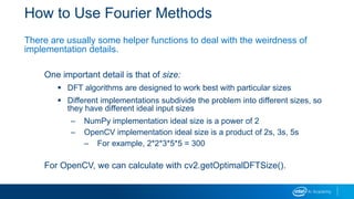
![FFT and DFT: p
We can convert to a function of a circle if
1. Our input is discrete and finite:
Map our values from [0, N-1] to points around the circle
Divide [0, 2p] into N parts
This is what we have with images
Images are discrete and finite
Edges of the images wrap to make a circle
2. Our input is discrete and repeating:
Do the exact same thing because the circle wraps around itself!](https://image.slidesharecdn.com/04imagetransformationsii-190218095700/85/04-image-transformations_ii-22-320.jpg)


![FFT and DFT: Forward
Forward: Data to circle
Input fdata([0,N-1]])
Output fcircles([0,N-1])
The input function tells us our data values
Input has N data values
Output has N circles
The output function tells us characteristics of the circles in our rewrites](https://image.slidesharecdn.com/04imagetransformationsii-190218095700/75/04-image-transformations_ii-19-2048.jpg)
![FFT and DFT: Backward
Backward: Circle to data
Input fcircles([0,N-1]])
Output fdata([0,N-1])
Here we are going from an input function in terms of circles to an output
function in terms of our data
Input has N circles
Output has N data values](https://image.slidesharecdn.com/04imagetransformationsii-190218095700/75/04-image-transformations_ii-20-2048.jpg)
![FFT and DFT: p
You might be worried that neither of these are necessarily functions of, or around, a
circle.
What is a function of a circle?
• A function of a circle is defined for each angle of a walk around a circle [0, 2p]
radians](https://image.slidesharecdn.com/04imagetransformationsii-190218095700/75/04-image-transformations_ii-21-2048.jpg)
![FFT and DFT: p
We can convert to a function of a circle if
1. Our input is discrete and finite:
Map our values from [0, N-1] to points around the circle
Divide [0, 2p] into N parts
This is what we have with images
Images are discrete and finite
Edges of the images wrap to make a circle
2. Our input is discrete and repeating:
Do the exact same thing because the circle wraps around itself!](https://image.slidesharecdn.com/04imagetransformationsii-190218095700/75/04-image-transformations_ii-22-2048.jpg)