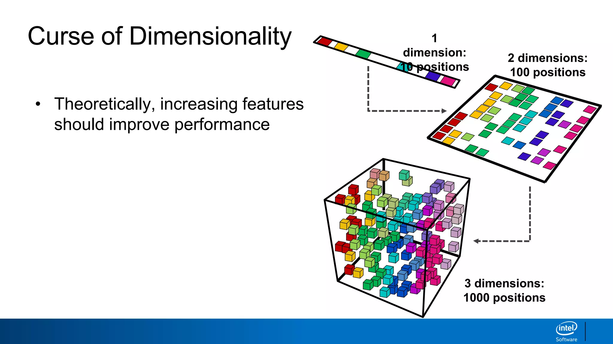
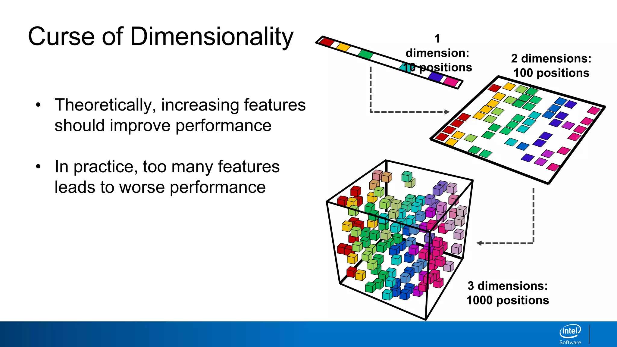
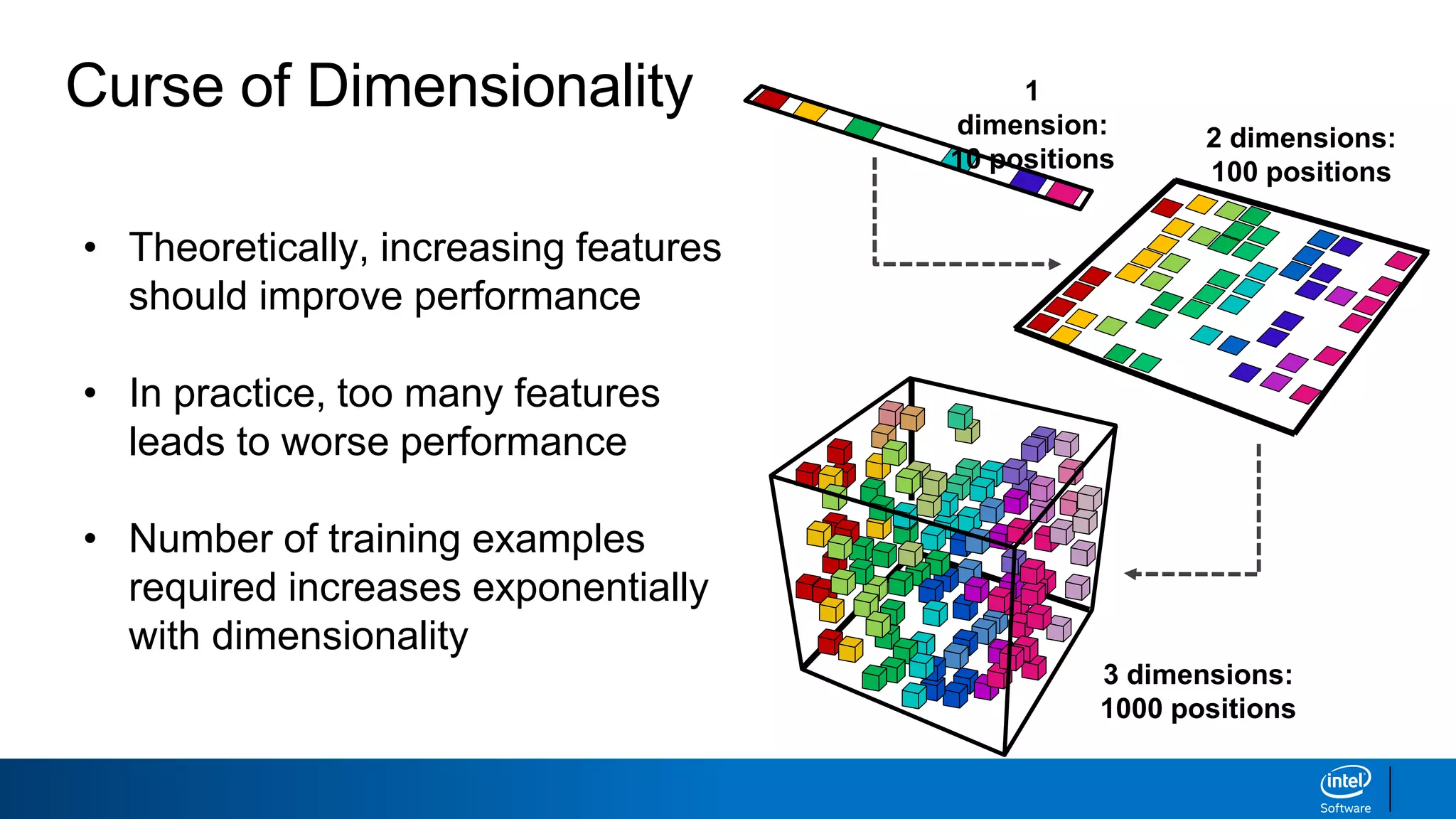
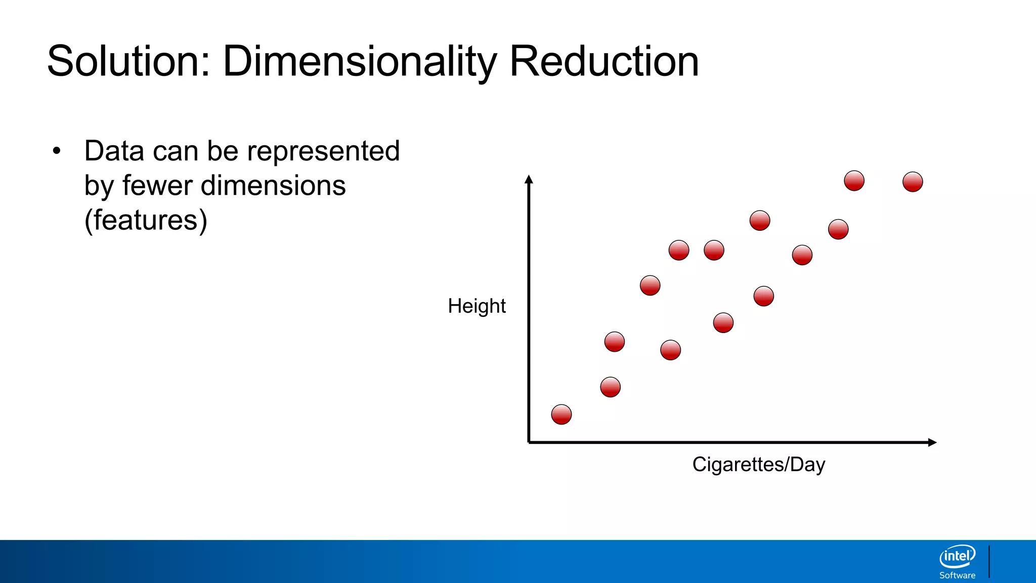
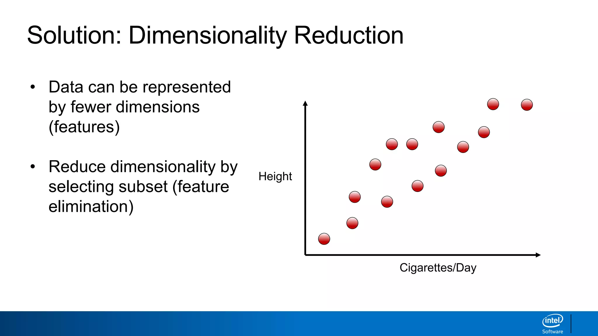
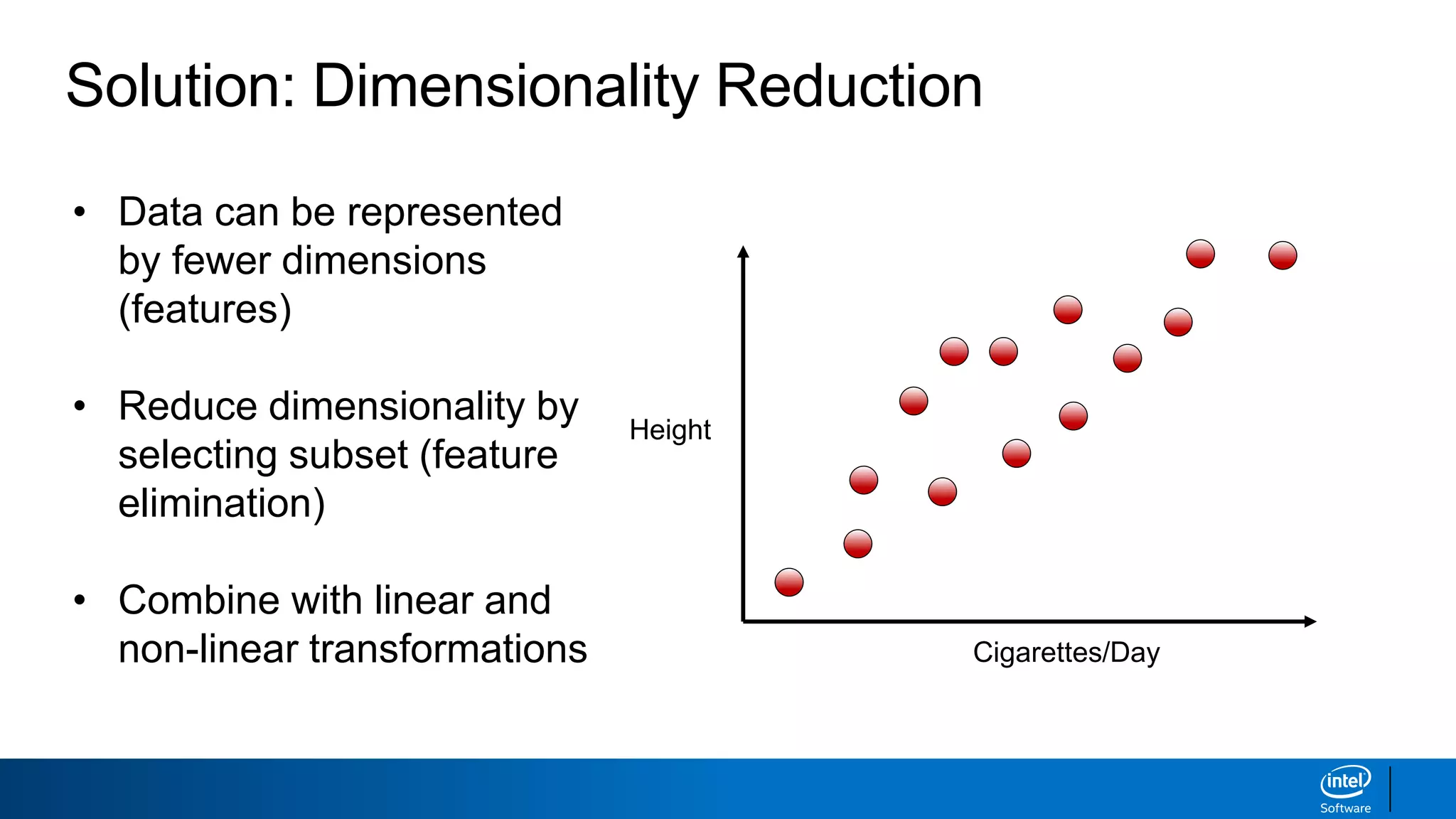
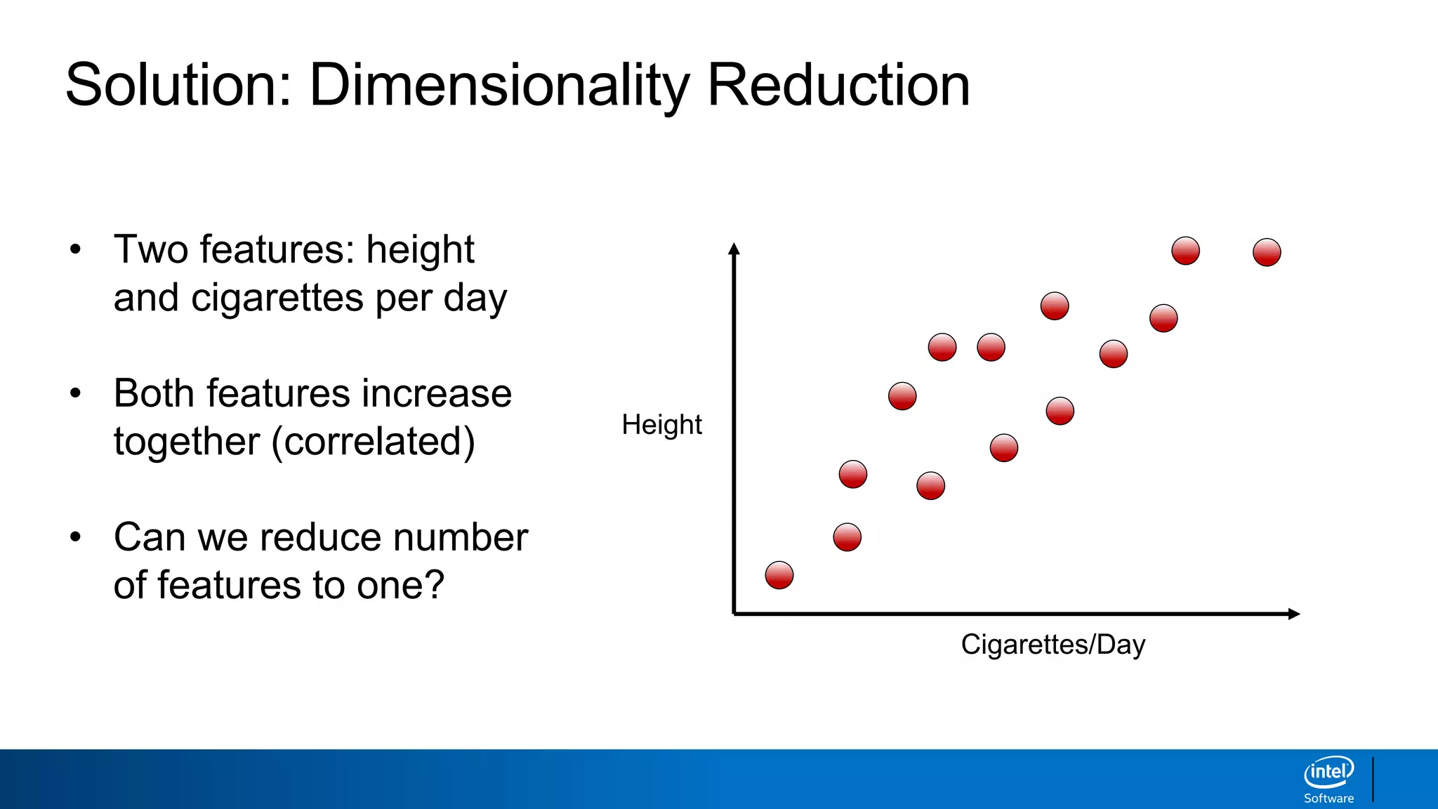
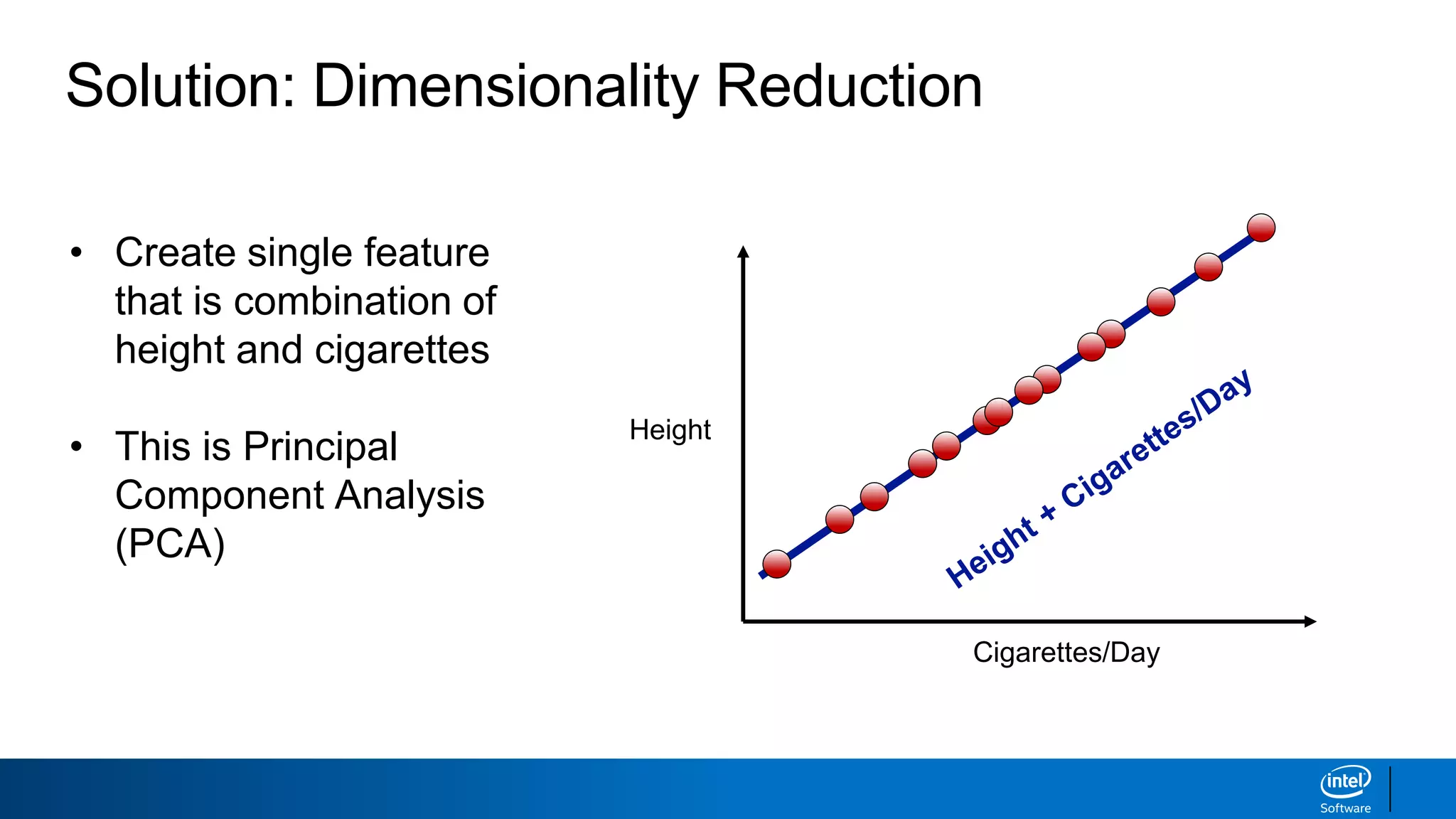
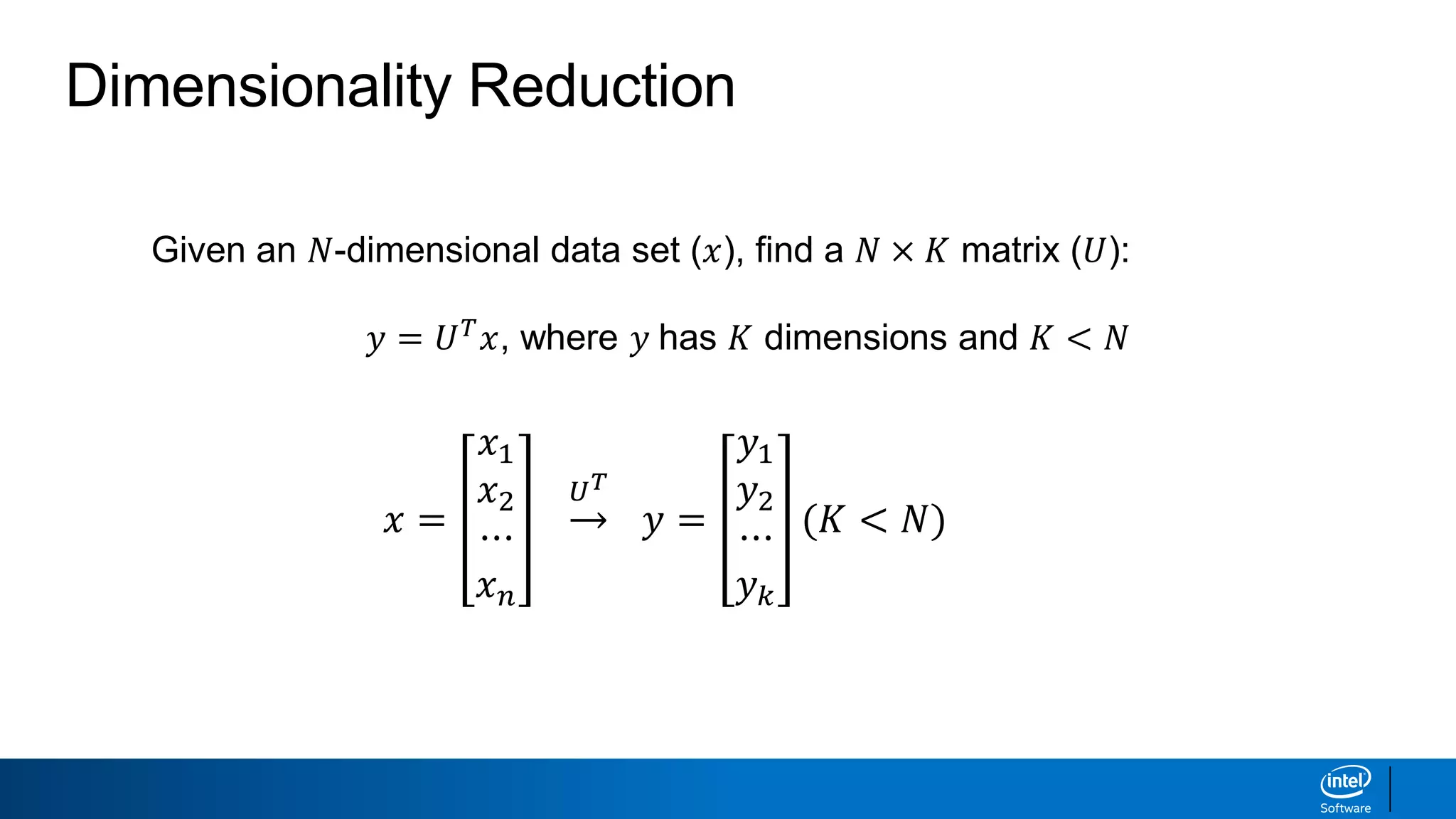
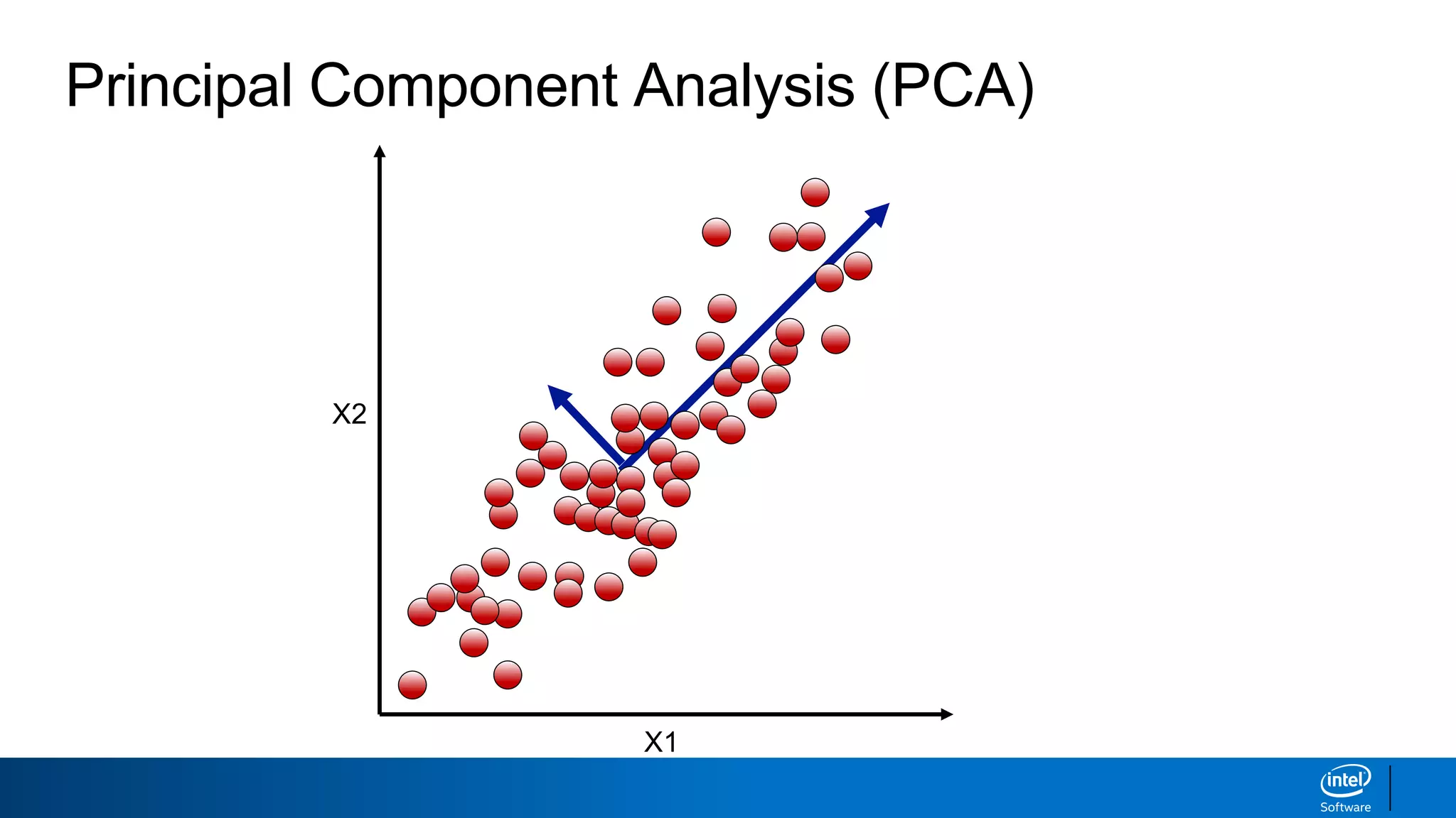
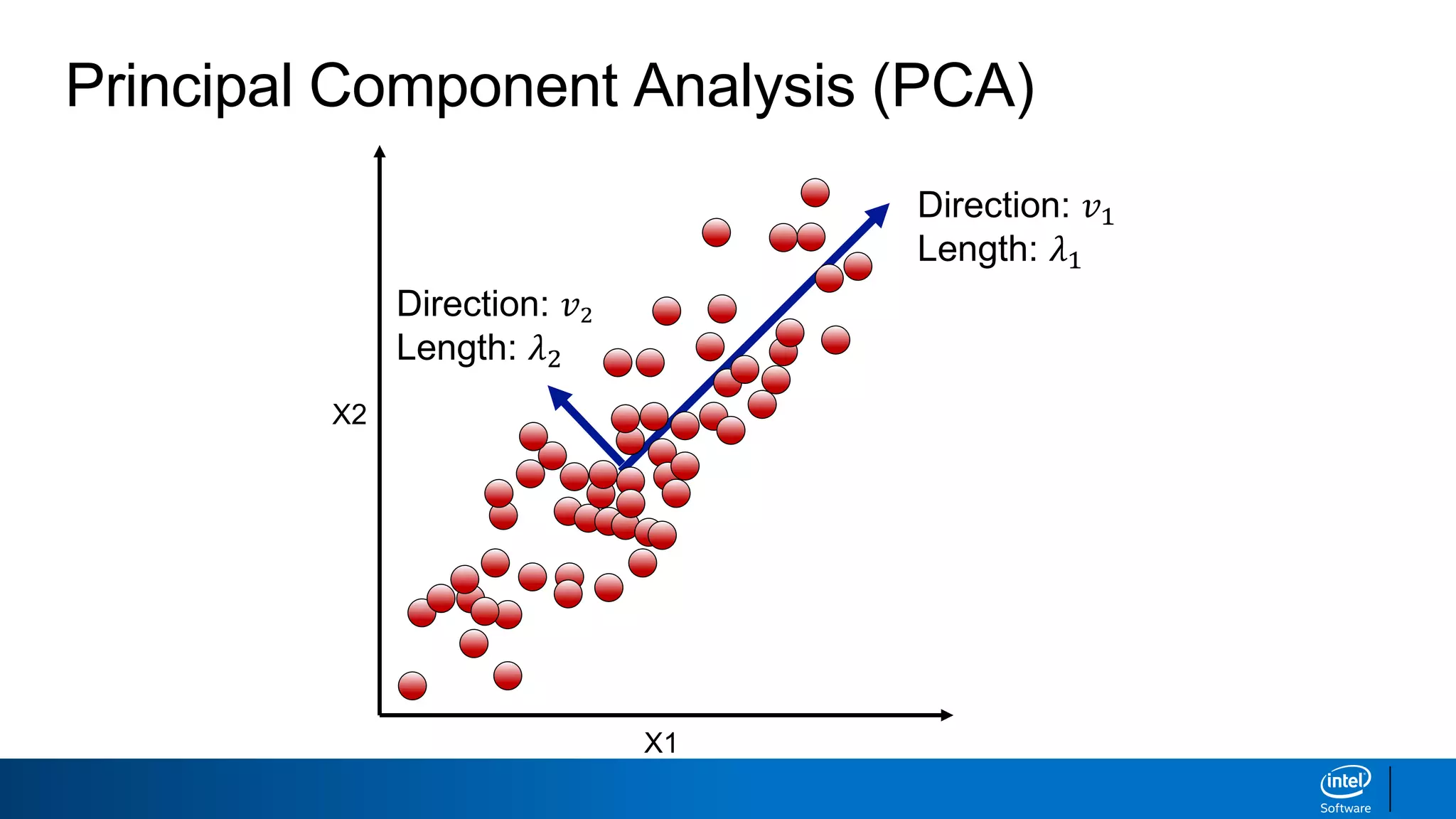
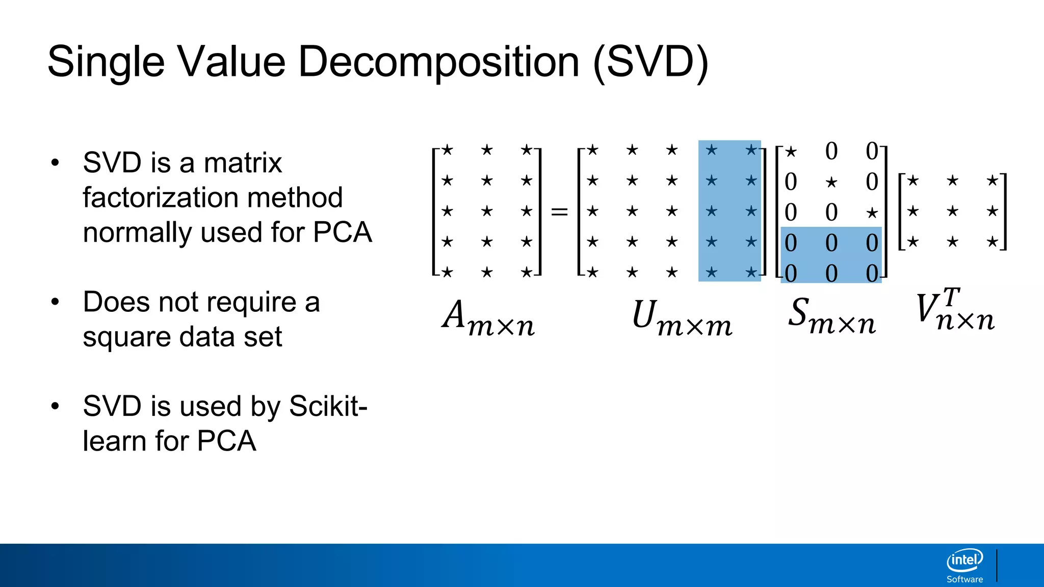
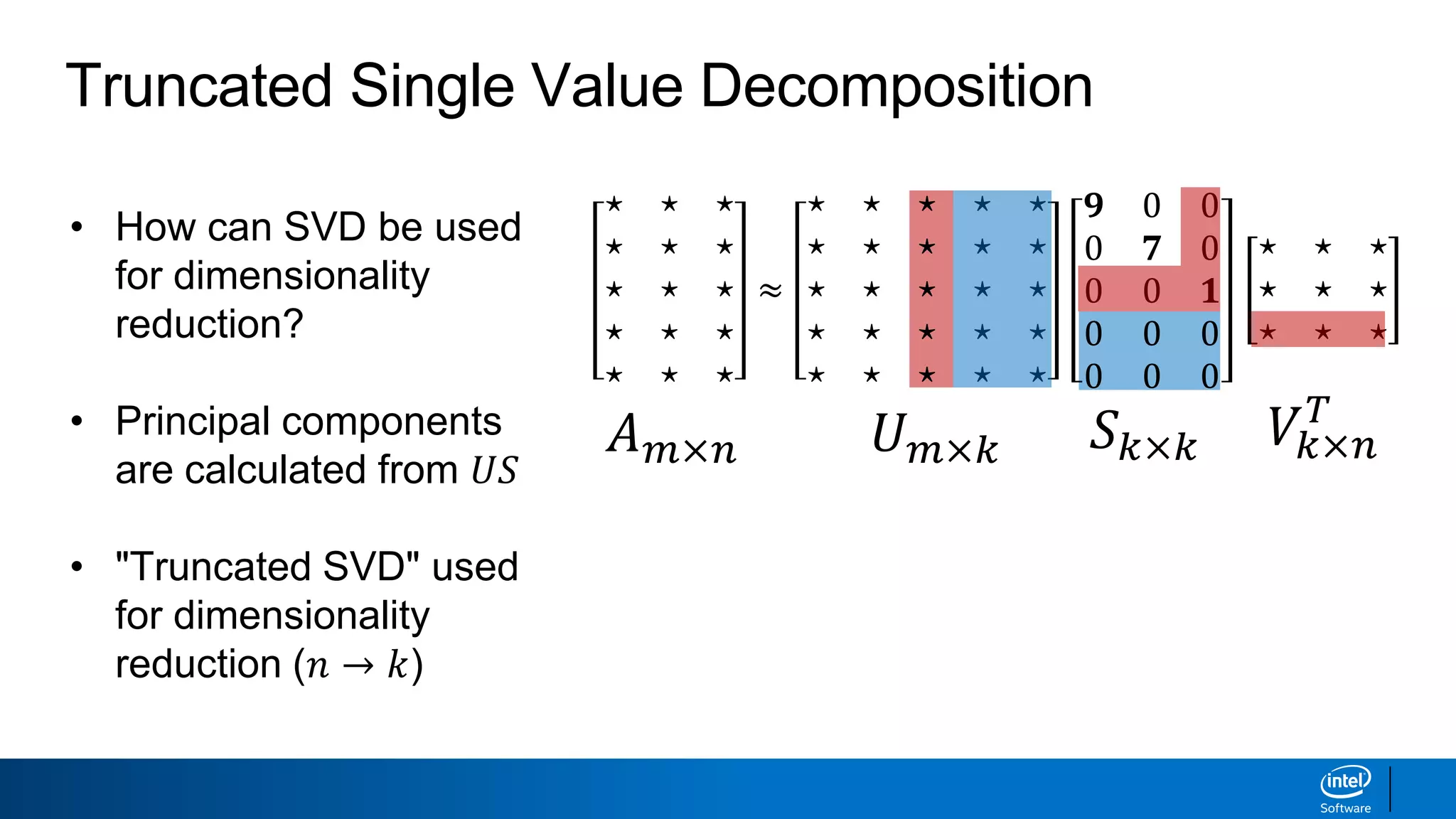
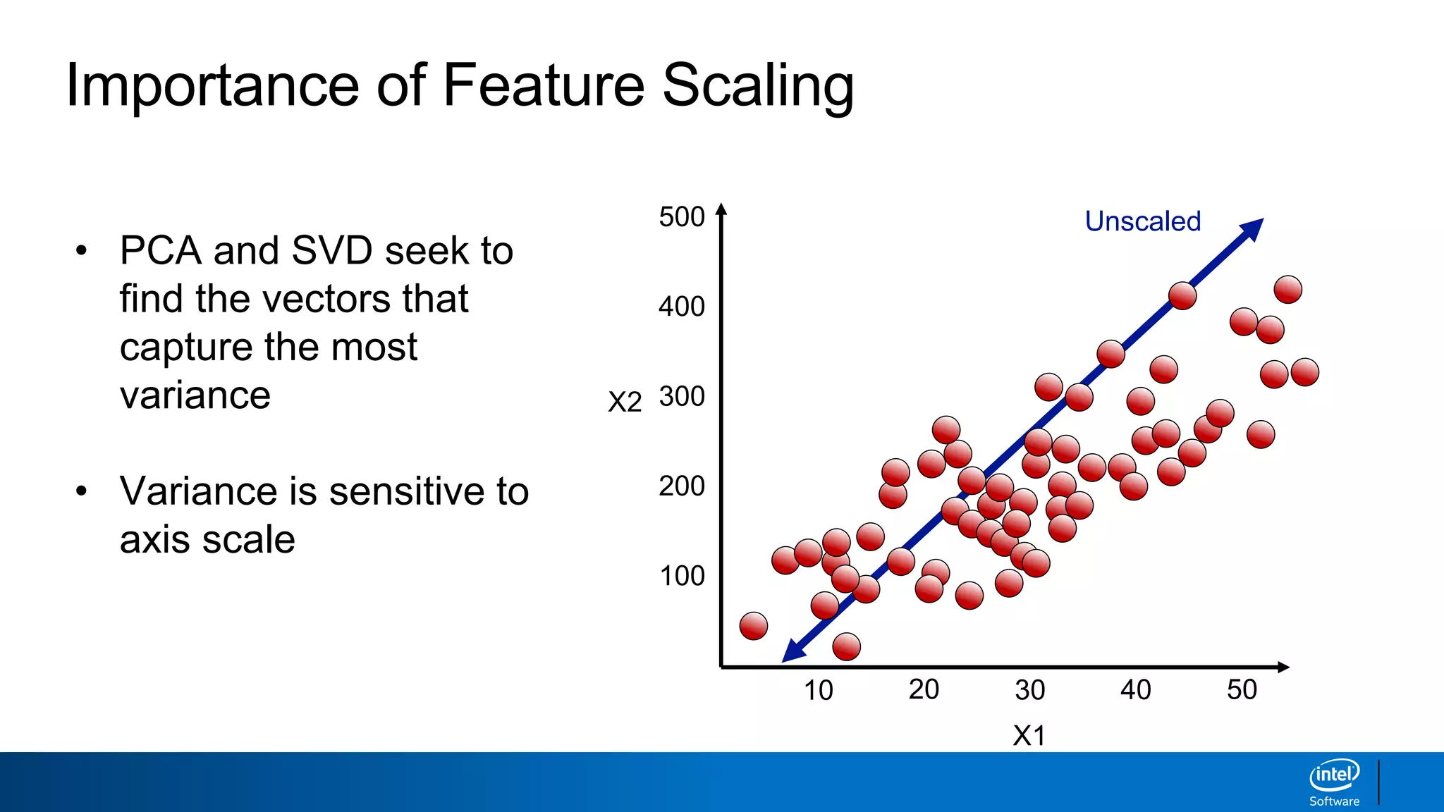
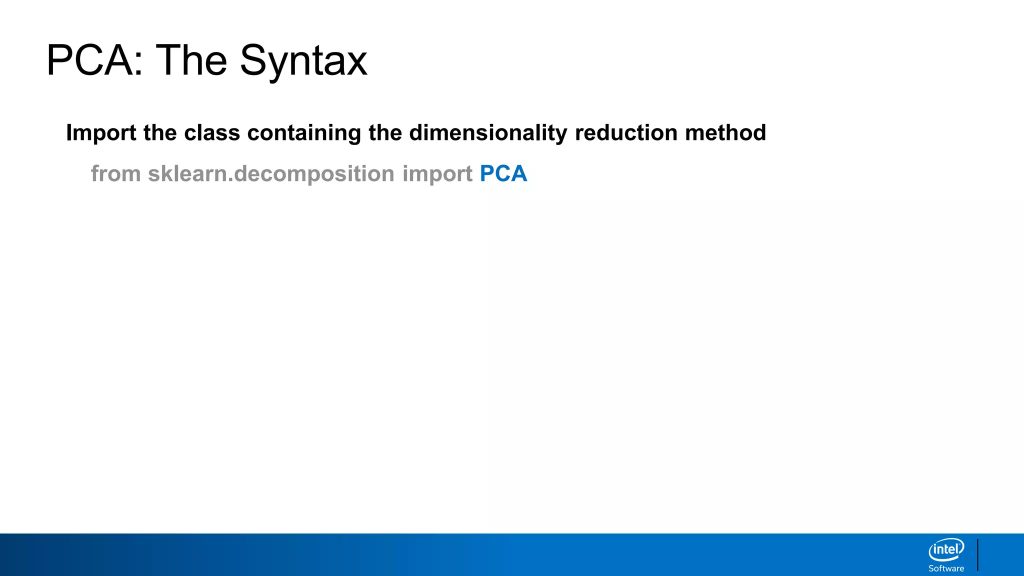
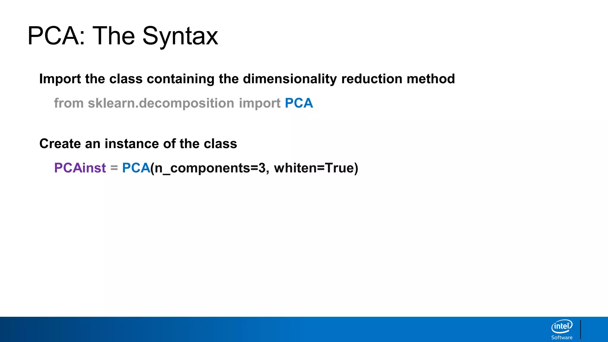
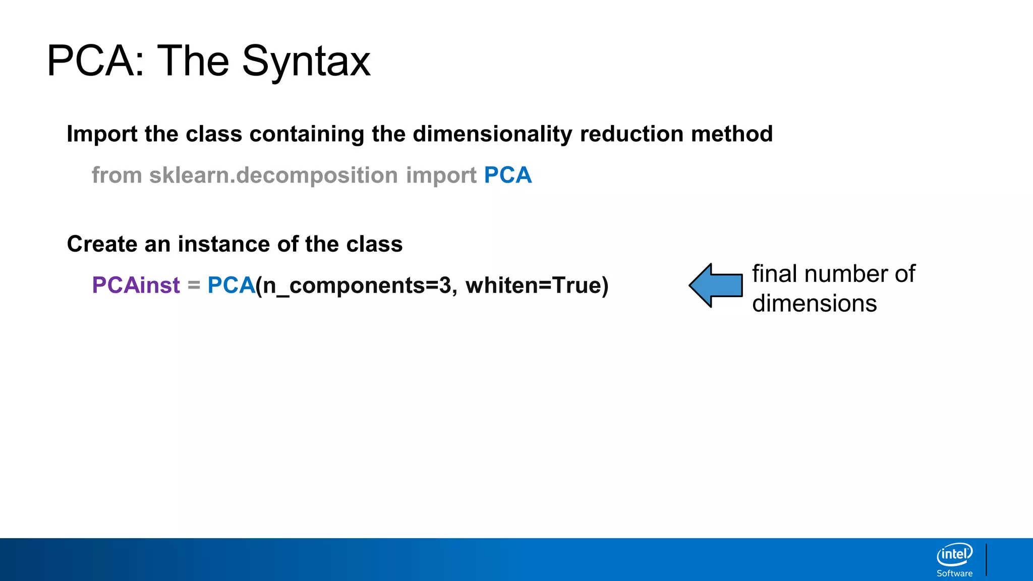
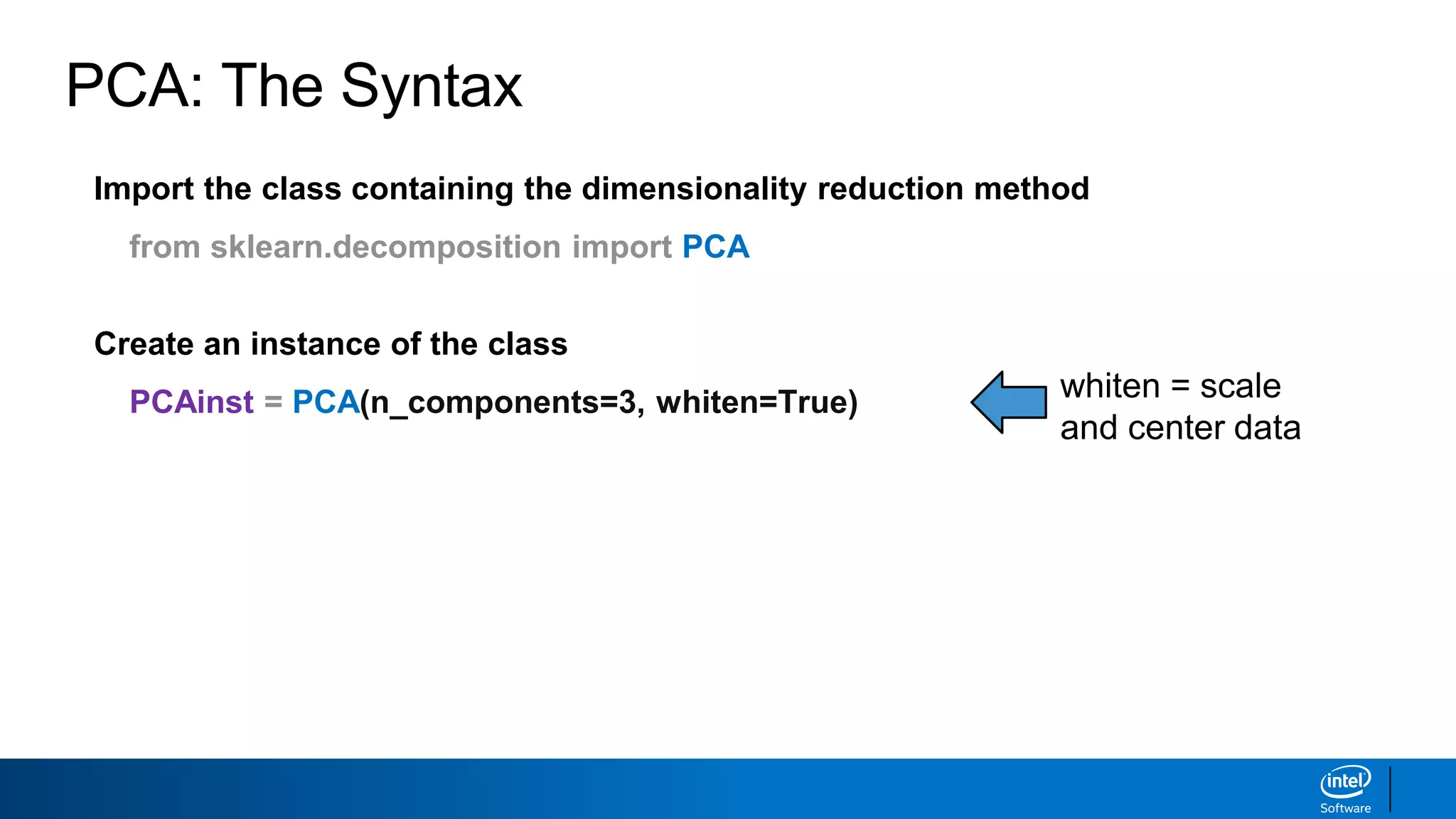
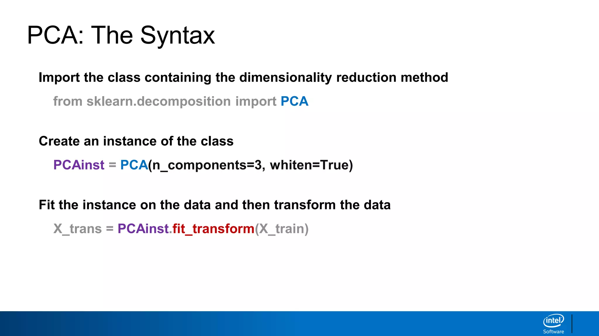
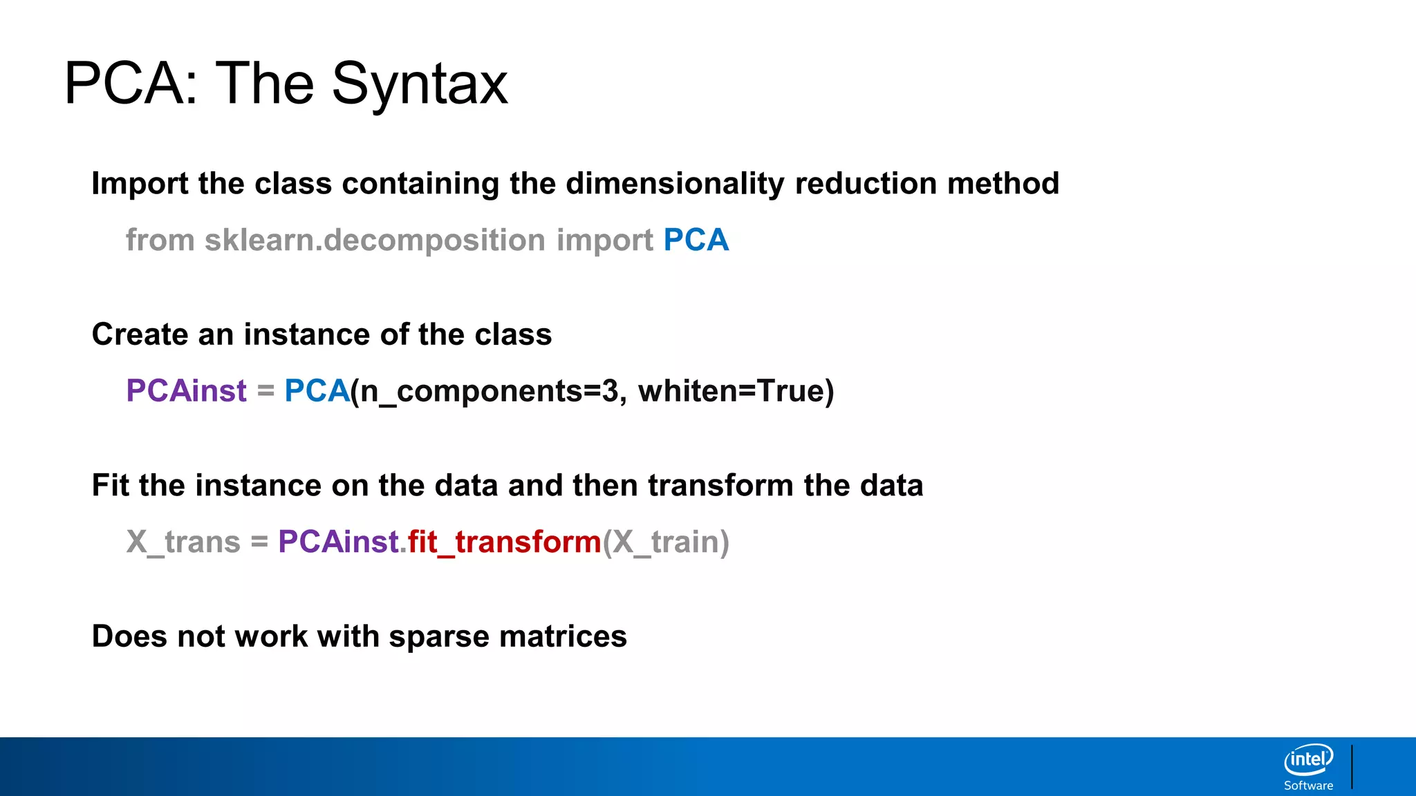
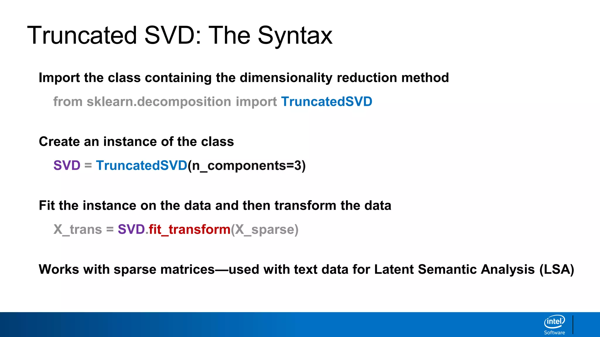
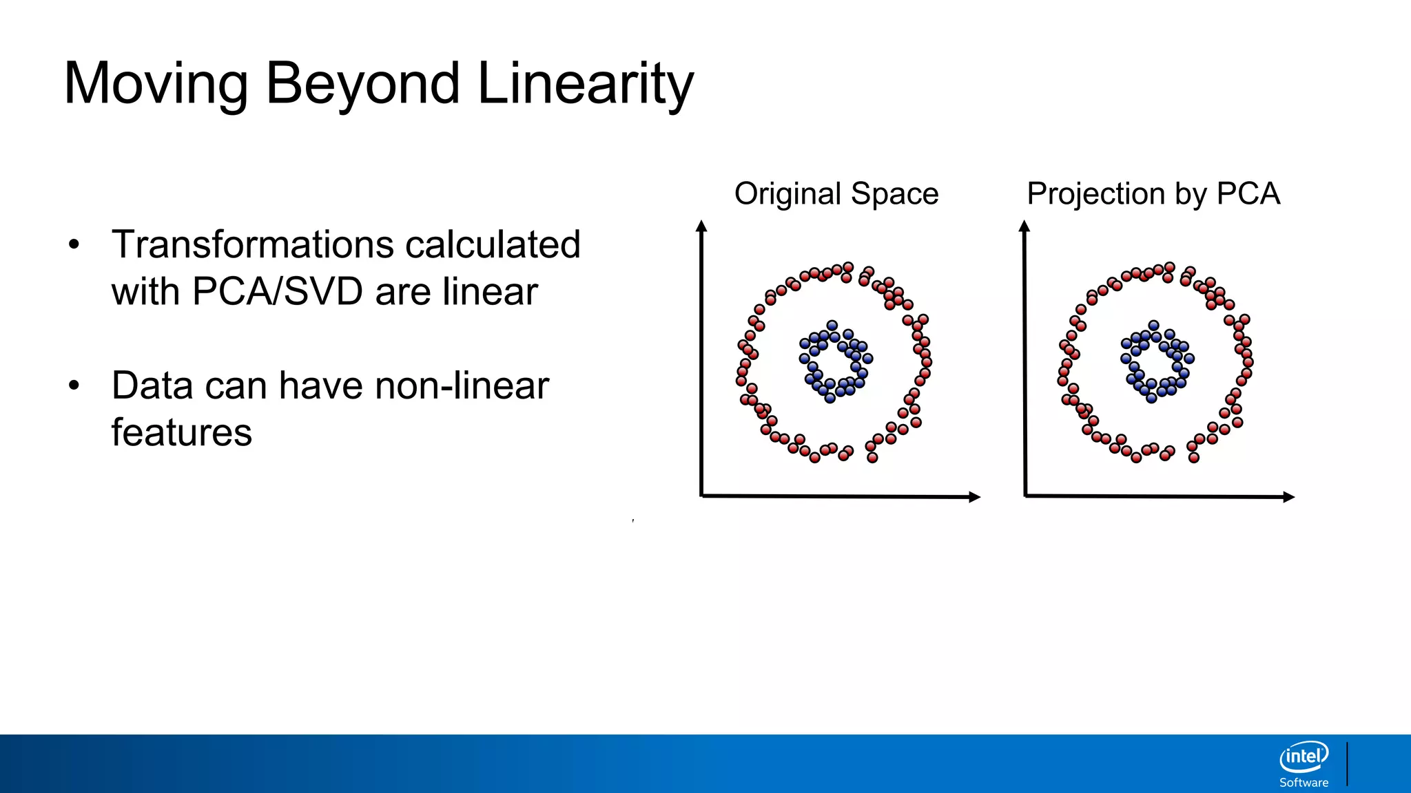
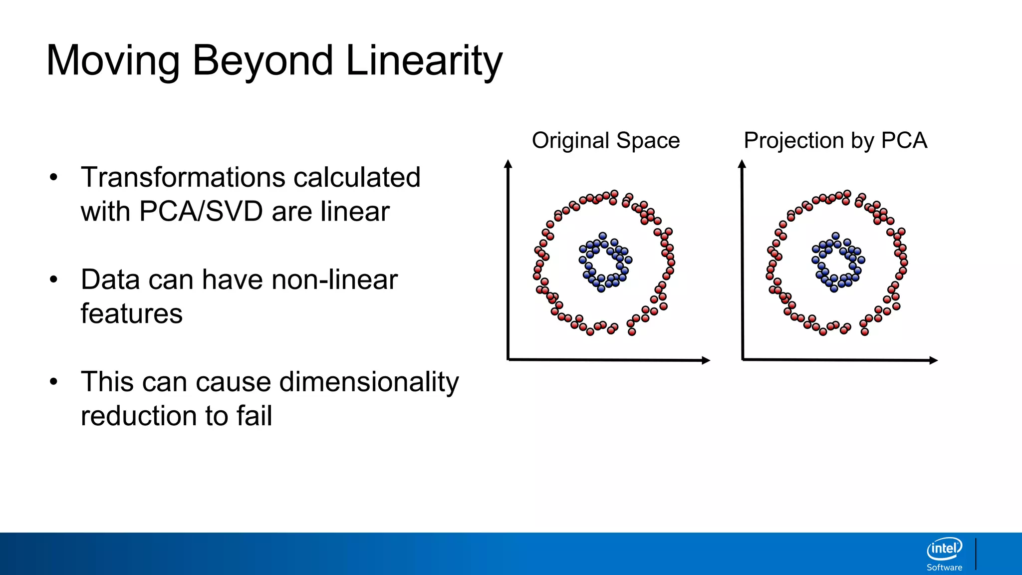
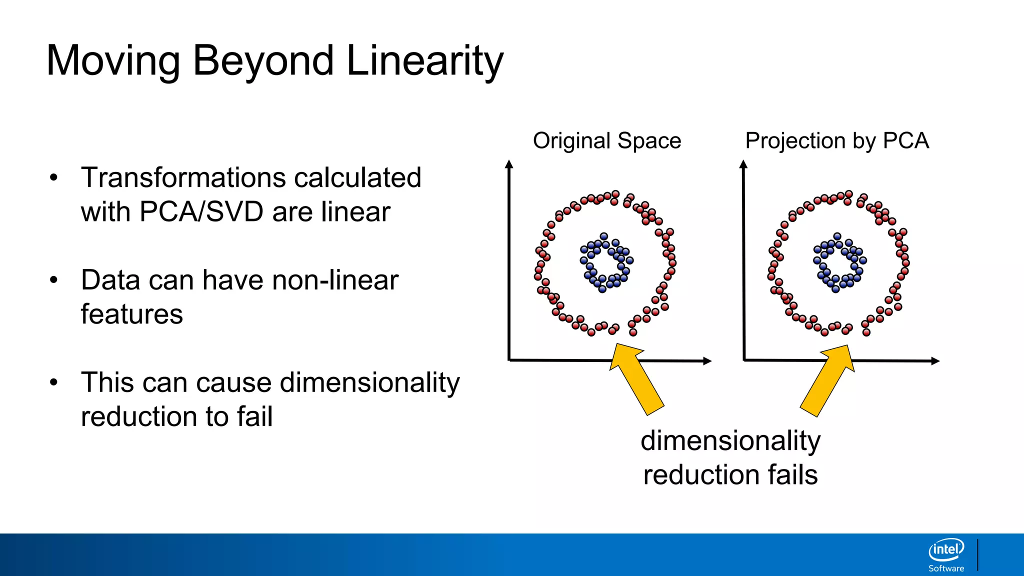
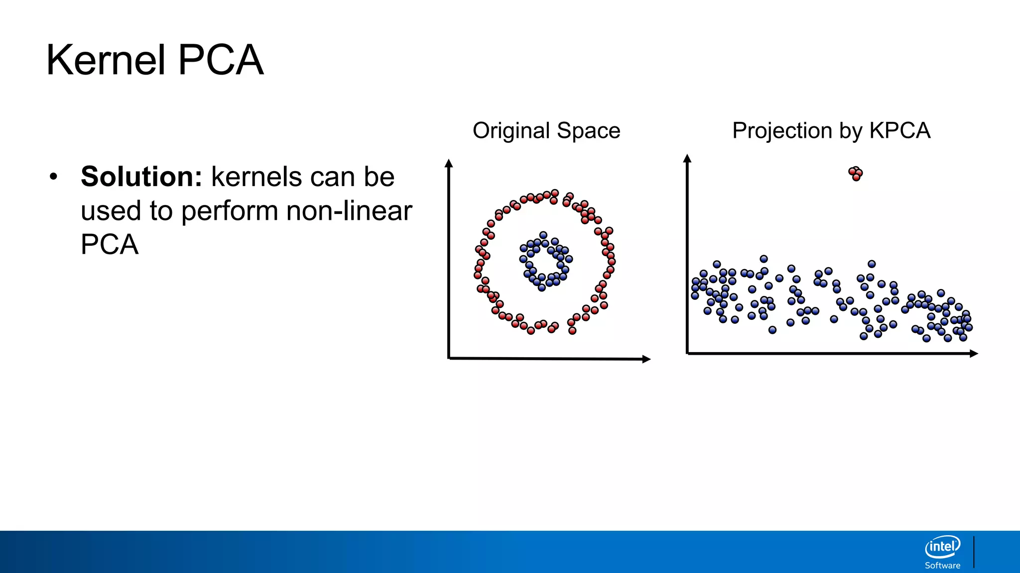
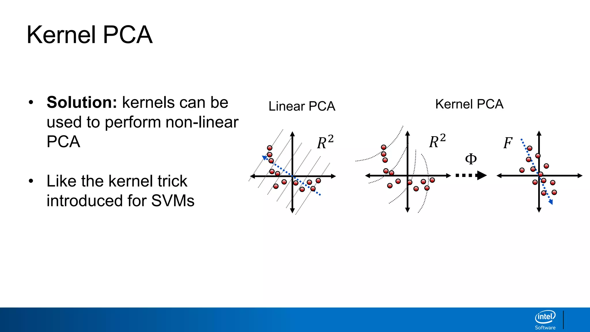
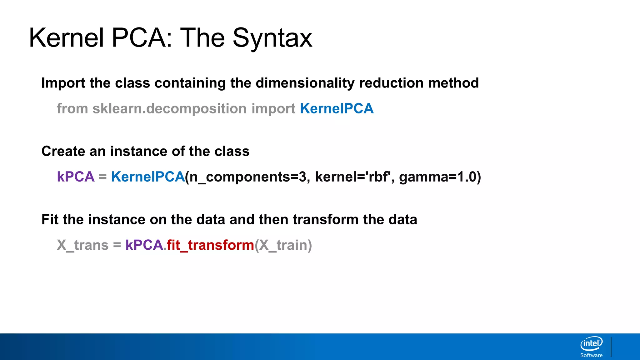
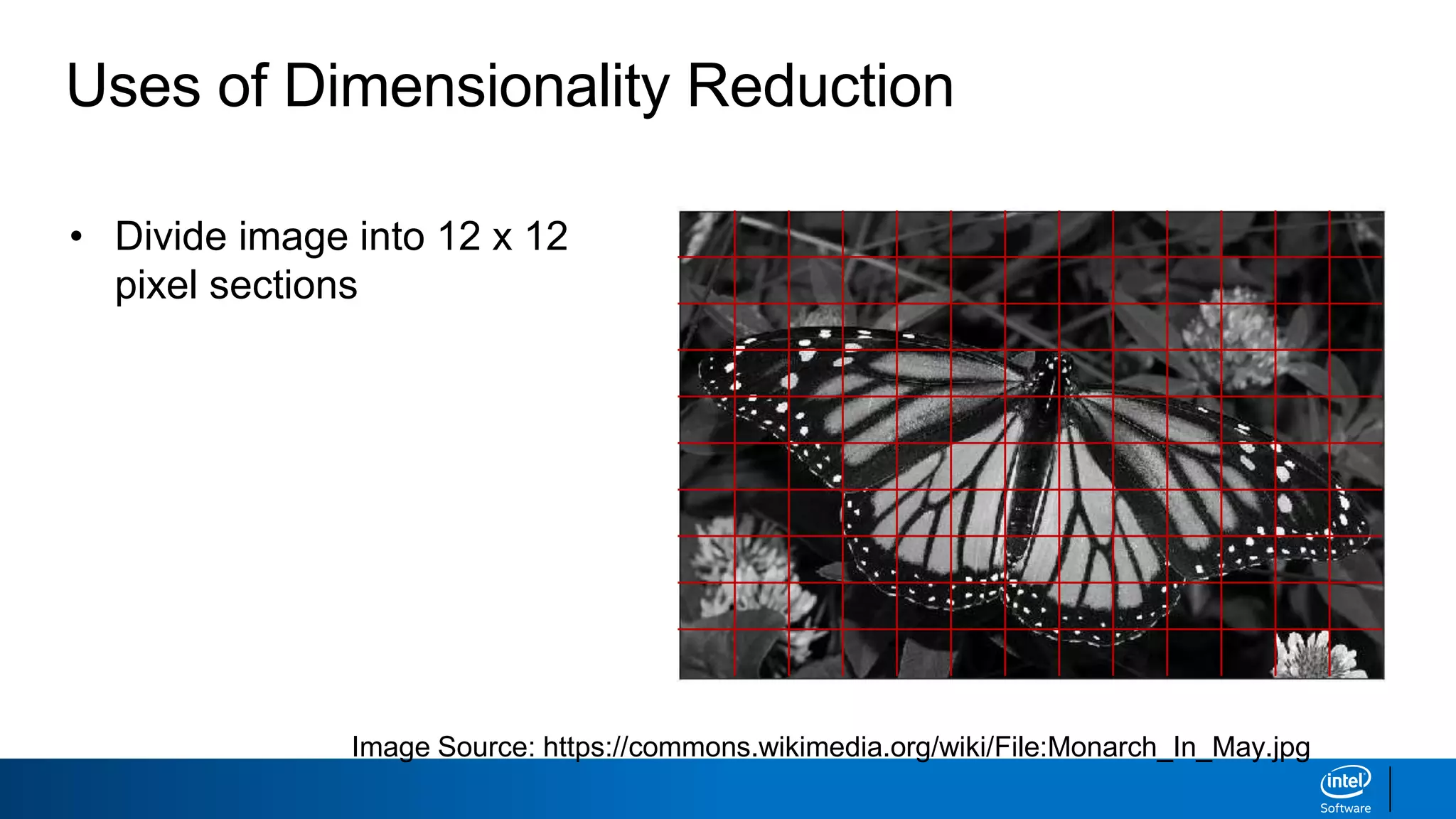
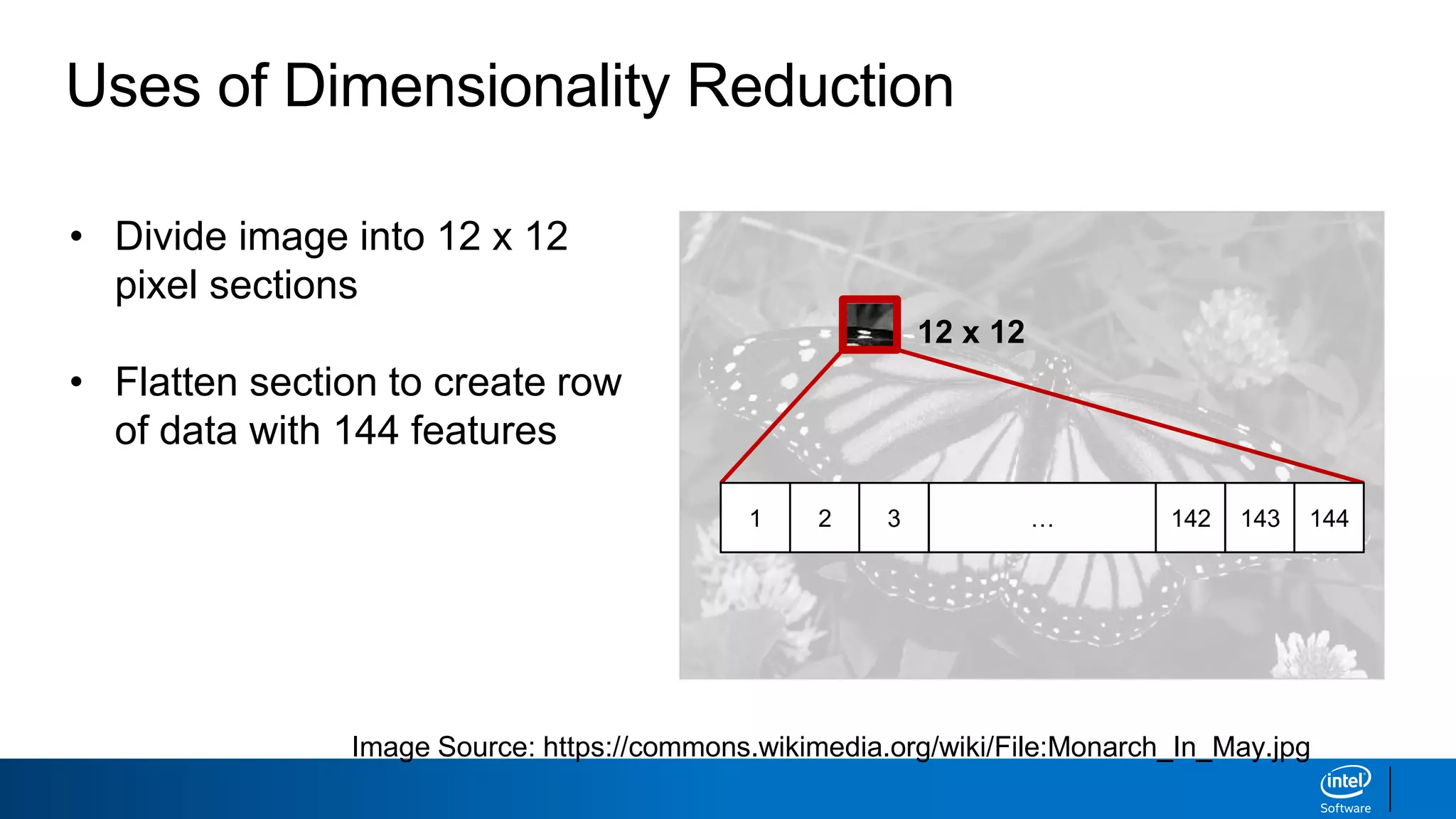
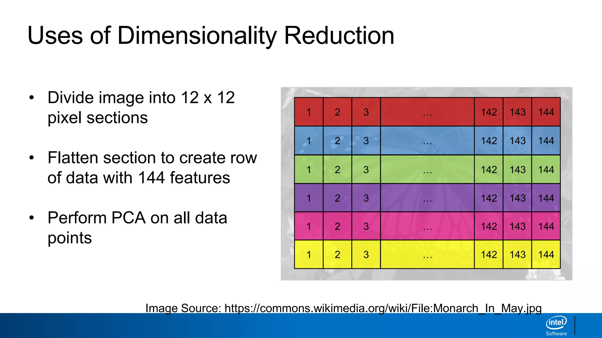
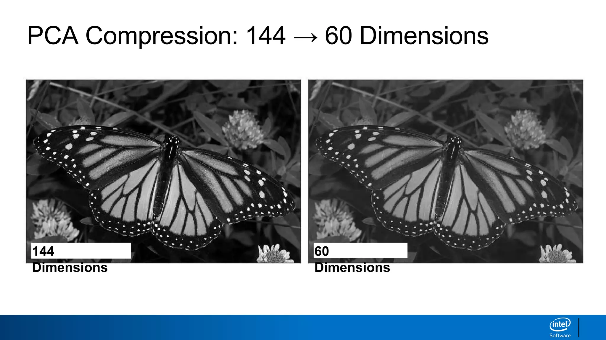
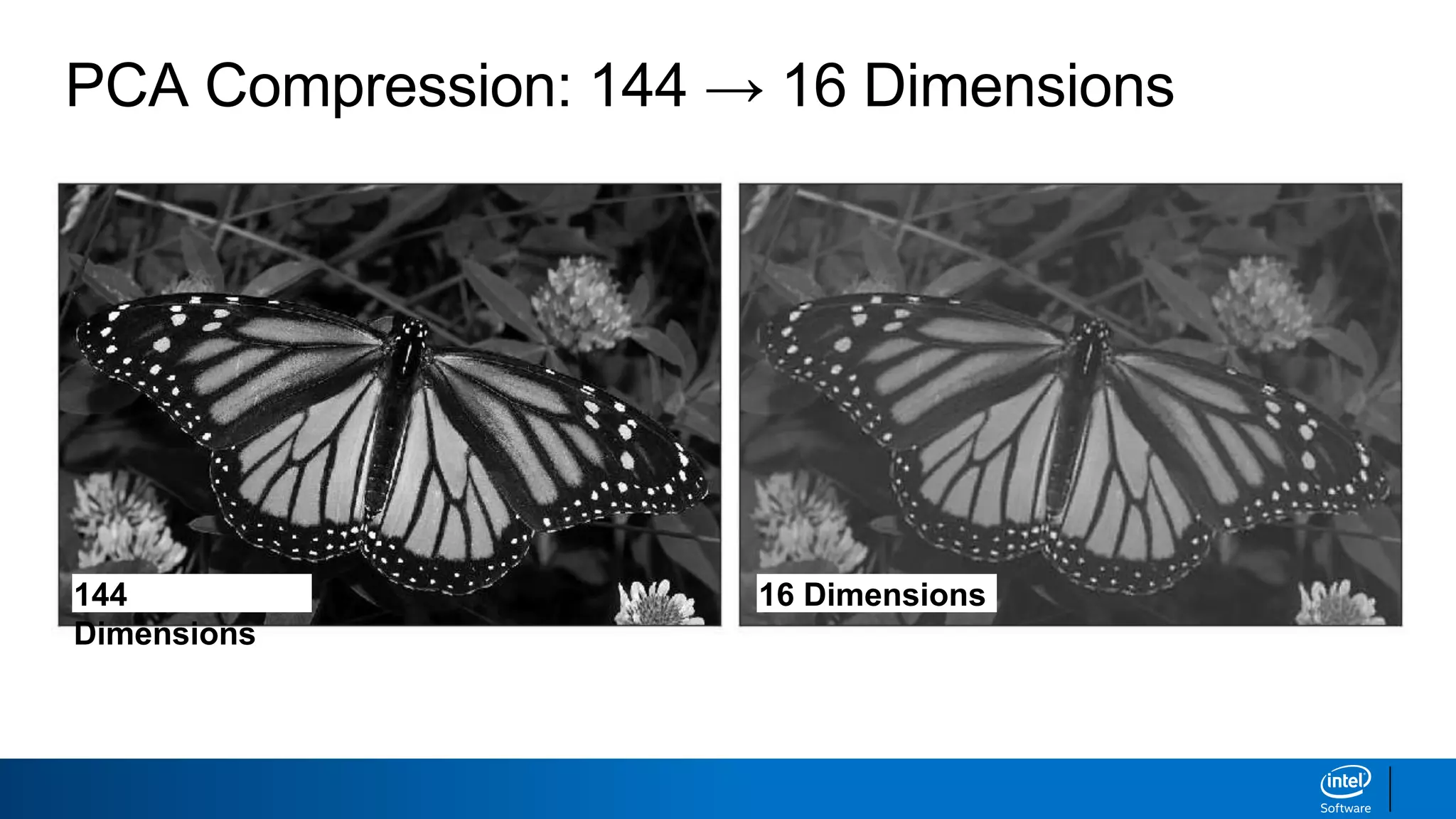
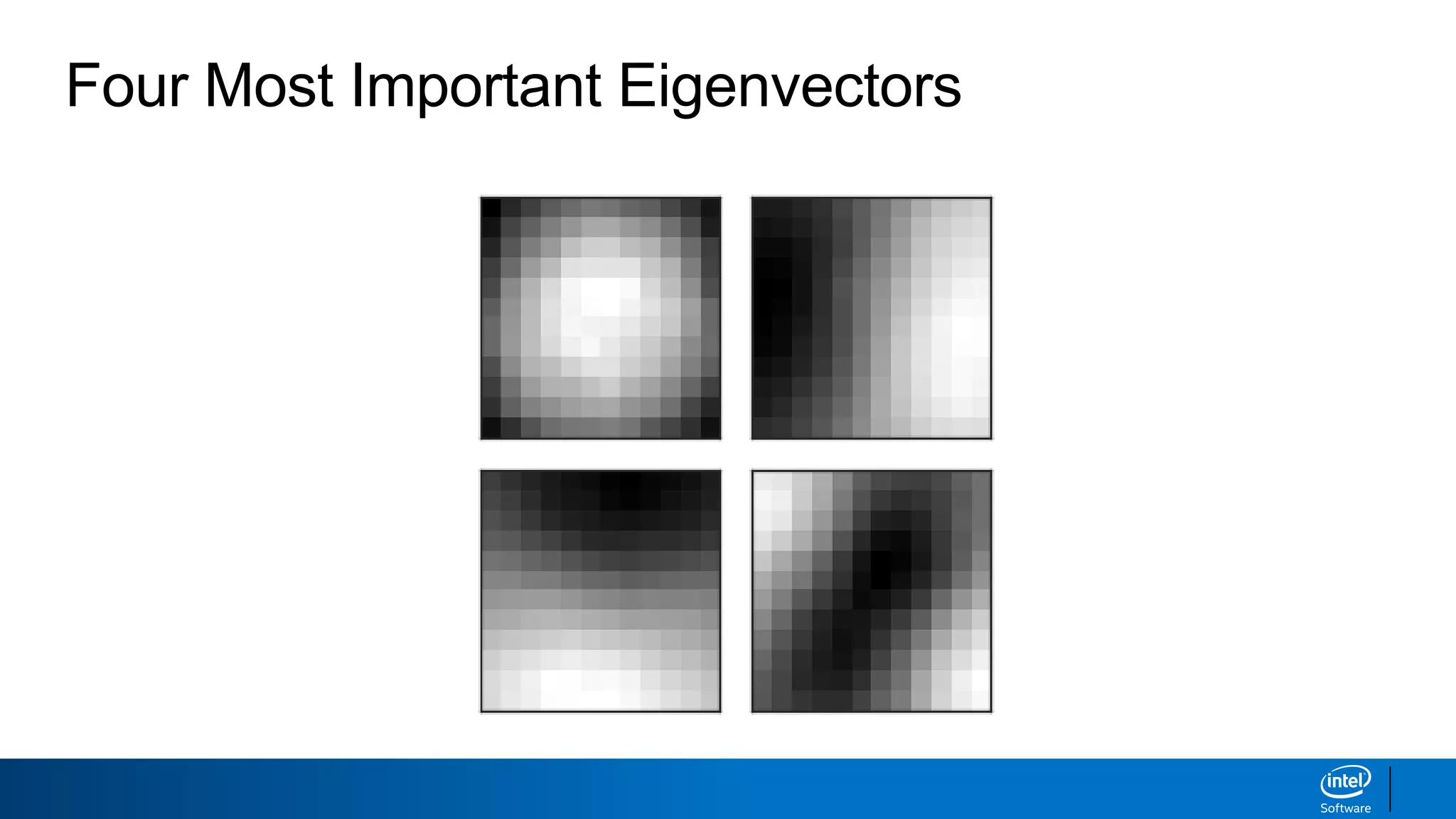
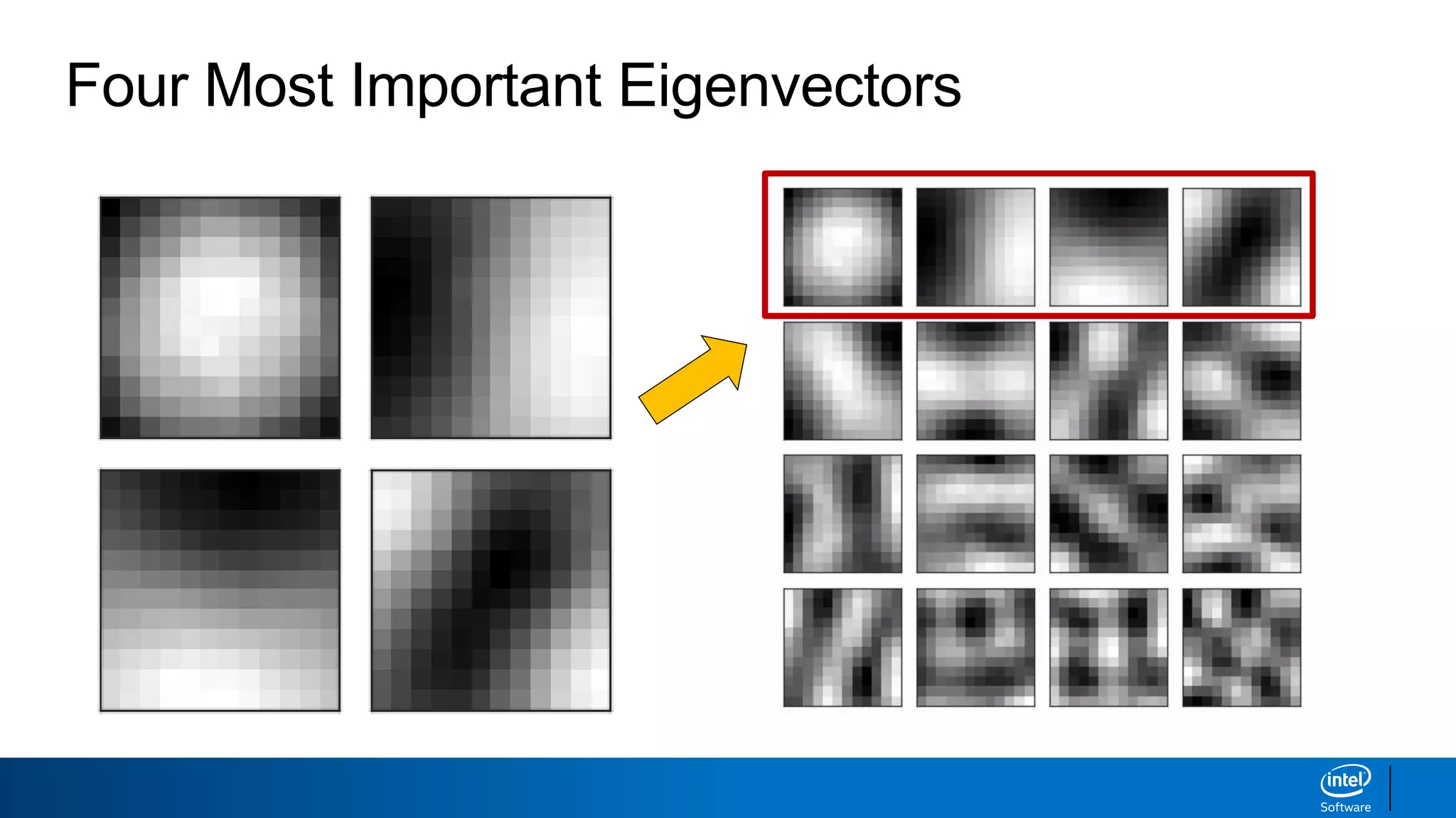
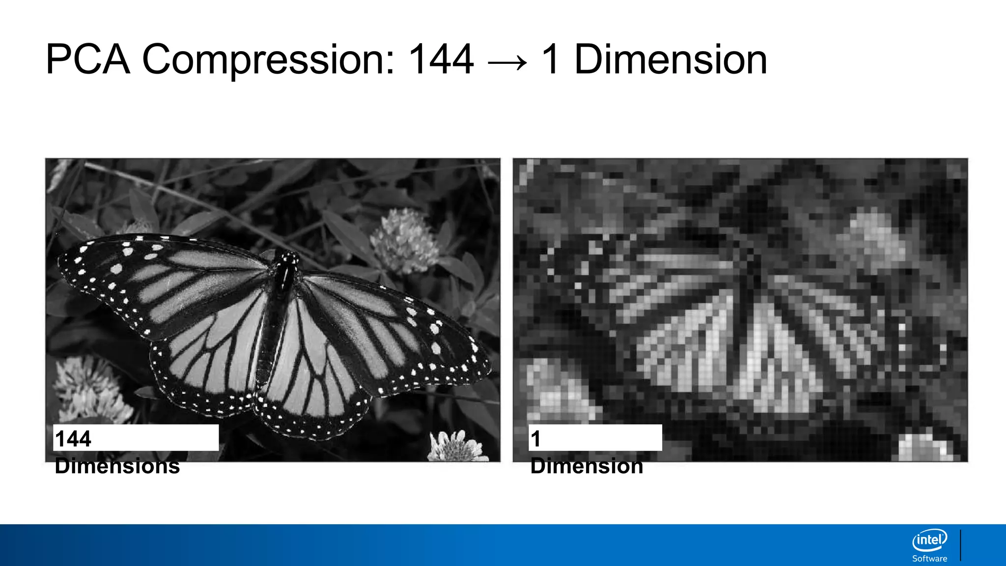
KEMBAR78
Ml10 dimensionality reduction-and_advanced_topics | PPTX
Dimensionality Reduction
Legal Notices and Disclaimers
This presentation is for informational purposes only. INTEL MAKES NO WARRANTIES,
EXPRESS OR IMPLIED, IN THIS SUMMARY.
Intel technologies’ features and benefits depend on system configuration and may require
enabled hardware, software or service activation. Performance varies depending on system
configuration. Check with your system manufacturer or retailer or learn more at intel.com.
This sample source code is released under the Intel Sample Source Code License Agreement.
Intel and the Intel logo are trademarks of Intel Corporation in the U.S. and/or other countries.
*Other names and brands may be claimed as the property of others.
Copyright © 2017, Intel Corporation. All rights reserved.
Curse of Dimensionality
• Theoretically, increasing features
should improve performance
• In practice, more features leads
to worse performance
• Number of training examples
required increases exponentially
with dimensionality
1
dimension:
10 positions
2 dimensions:
100 positions
3 dimensions:
1000 positions
Curse of Dimensionality
• Theoretically, increasing features
should improve performance
• In practice, too many features
leads to worse performance
1
dimension:
10 positions
2 dimensions:
100 positions
3 dimensions:
1000 positions
Curse of Dimensionality
• Theoretically, increasing features
should improve performance
• In practice, too many features
leads to worse performance
• Number of training examples
required increases exponentially
with dimensionality
1
dimension:
10 positions
2 dimensions:
100 positions
3 dimensions:
1000 positions
Solution: Dimensionality Reduction
• Data can be represented
by fewer dimensions
(features)
• Reduce dimensionality by
selecting subset (feature
elimination)
• Combine with linear and
non-linear transformations
Height
Cigarettes/Day
Solution: Dimensionality Reduction
• Data can be represented
by fewer dimensions
(features)
• Reduce dimensionality by
selecting subset (feature
elimination)
• Combine with linear and
non-linear transformations
Height
Cigarettes/Day
Solution: Dimensionality Reduction
• Data can be represented
by fewer dimensions
(features)
• Reduce dimensionality by
selecting subset (feature
elimination)
• Combine with linear and
non-linear transformations
Height
Cigarettes/Day
Solution: Dimensionality Reduction
• Two features: height
and cigarettes per day
• Both features increase
together (correlated)
• Can we reduce number
of features to one?
Height
Cigarettes/Day
Solution: Dimensionality Reduction
• Two features: height
and cigarettes per day
• Both features increase
together (correlated)
• Can we reduce number
of features to one?
Height
Cigarettes/Day
Solution: Dimensionality Reduction
• Two features: height
and cigarettes per day
• Both features increase
together (correlated)
• Can we reduce number
of features to one?
Height
Cigarettes/Day
Solution: Dimensionality Reduction
• Two features: height
and cigarettes per day
• Both features increase
together (correlated)
• Can we reduce number
of features to one?
Height
Cigarettes/Day
Solution: Dimensionality Reduction
• Create single feature
that is combination of
height and cigarettes
• This is Principal
Component Analysis
(PCA)
Height
Cigarettes/Day
Solution: Dimensionality Reduction
• Create single feature
that is combination of
height and cigarettes
• This is Principal
Component Analysis
(PCA)
Dimensionality Reduction
Given an 𝑁-dimensional data set (𝑥), find a 𝑁 × 𝐾 matrix (𝑈):
𝑦 = 𝑈 𝑇
𝑥, where 𝑦 has 𝐾 dimensions and 𝐾 < 𝑁
𝑥 =
𝑥1
𝑥2
⋯
𝑥 𝑛
𝑈 𝑇
𝑦 =
𝑦1
𝑦2
⋯
𝑦 𝑘
(𝐾 < 𝑁)
Principal Component Analysis (PCA)
X2
X1
Principal Component Analysis (PCA)
X2
X1
Principal Component Analysis (PCA)
X2
X1
Principal Component Analysis (PCA)
X2
X1
Direction: 𝑣1
Length: 𝜆1
Direction: 𝑣2
Length: 𝜆2
• SVD is a matrix
factorization method
normally used for PCA
• Does not require a
square data set
• SVD is used by Scikit-
learn for PCA
Single Value Decomposition (SVD)
𝐴 𝑚×𝑛 𝑈 𝑚×𝑚 𝑆 𝑚×𝑛 𝑉𝑛×𝑛
𝑇
⋆ ⋆ ⋆
⋆ ⋆ ⋆
⋆ ⋆ ⋆
⋆ ⋆ ⋆
⋆ ⋆ ⋆
=
⋆ ⋆ ⋆ ⋆ ⋆
⋆ ⋆ ⋆ ⋆ ⋆
⋆ ⋆ ⋆ ⋆ ⋆
⋆ ⋆ ⋆ ⋆ ⋆
⋆ ⋆ ⋆ ⋆ ⋆
⋆ 0 0
0 ⋆ 0
0 0 ⋆
0 0 0
0 0 0
⋆ ⋆ ⋆
⋆ ⋆ ⋆
⋆ ⋆ ⋆
• How can SVD be used
for dimensionality
reduction?
• Principal components
are calculated from 𝑈𝑆
• "Truncated SVD" used
for dimensionality
reduction (𝑛 → 𝑘)
Truncated Single Value Decomposition
𝐴 𝑚×𝑛 𝑈 𝑚×𝑘 𝑆 𝑘×𝑘 𝑉𝑘×𝑛
𝑇
⋆ ⋆ ⋆
⋆ ⋆ ⋆
⋆ ⋆ ⋆
⋆ ⋆ ⋆
⋆ ⋆ ⋆
≈
⋆ ⋆ ⋆ ⋆ ⋆
⋆ ⋆ ⋆ ⋆ ⋆
⋆ ⋆ ⋆ ⋆ ⋆
⋆ ⋆ ⋆ ⋆ ⋆
⋆ ⋆ ⋆ ⋆ ⋆
𝟗 0 0
0 𝟕 0
0 0 𝟏
0 0 0
0 0 0
⋆ ⋆ ⋆
⋆ ⋆ ⋆
⋆ ⋆ ⋆
• PCA and SVD seek to
find the vectors that
capture the most
variance
• Variance is sensitive to
axis scale
• Must scale data!
Importance of Feature Scaling
X2
X1
100
200
300
400
500
10 20 30 40 50
Unscaled
• PCA and SVD seek to
find the vectors that
capture the most
variance
• Variance is sensitive to
axis scale
• Must scale data!
X2
X1
10
20
30
40
50
10 20 30 40 50
Unscaled
Scaled
Importance of Feature Scaling
Import the class containing the dimensionality reduction method
from sklearn.decomposition import PCA
Create an instance of the class
PCAinst = PCA(n_components=3, whiten=True)
Fit the instance on the data and then transform the data
X_trans = PCAinst.fit_transform(X_train)
Does not work with sparse matrices
PCA: The Syntax
Import the class containing the dimensionality reduction method
from sklearn.decomposition import PCA
Create an instance of the class
PCAinst = PCA(n_components=3, whiten=True)
PCA: The Syntax
Import the class containing the dimensionality reduction method
from sklearn.decomposition import PCA
Create an instance of the class
PCAinst = PCA(n_components=3, whiten=True) final number of
dimensions
PCA: The Syntax
Import the class containing the dimensionality reduction method
from sklearn.decomposition import PCA
Create an instance of the class
PCAinst = PCA(n_components=3, whiten=True) whiten = scale
and center data
PCA: The Syntax
Import the class containing the dimensionality reduction method
from sklearn.decomposition import PCA
Create an instance of the class
PCAinst = PCA(n_components=3, whiten=True)
Fit the instance on the data and then transform the data
X_trans = PCAinst.fit_transform(X_train)
Does not work with sparse matrices
PCA: The Syntax
Import the class containing the dimensionality reduction method
from sklearn.decomposition import PCA
Create an instance of the class
PCAinst = PCA(n_components=3, whiten=True)
Fit the instance on the data and then transform the data
X_trans = PCAinst.fit_transform(X_train)
Does not work with sparse matrices
PCA: The Syntax
Truncated SVD: The Syntax
Import the class containing the dimensionality reduction method
from sklearn.decomposition import TruncatedSVD
Create an instance of the class
SVD = TruncatedSVD(n_components=3)
Fit the instance on the data and then transform the data
X_trans = SVD.fit_transform(X_sparse)
Works with sparse matrices—used with text data for Latent Semantic Analysis (LSA)
does not
center data
Truncated SVD: The Syntax
• Transformations calculated
with PCA/SVD are linear
• Data can have non-linear
features
• This can cause dimensionality
reduction to fail
Moving Beyond Linearity
Original Space Projection by PCA
• Transformations calculated
with PCA/SVD are linear
• Data can have non-linear
features
• This can cause dimensionality
reduction to fail
Moving Beyond Linearity
Original Space Projection by PCA
• Transformations calculated
with PCA/SVD are linear
• Data can have non-linear
features
• This can cause dimensionality
reduction to fail
Moving Beyond Linearity
Original Space Projection by PCA
dimensionality
reduction fails
• Solution: kernels can be
used to perform non-linear
PCA
• Like the kernel trick
introduced for SVMs
Kernel PCA
Original Space Projection by KPCA
Kernel PCA
Linear PCA
𝑅2 𝑅2
Φ
𝐹
Kernel PCA• Solution: kernels can be
used to perform non-linear
PCA
• Like the kernel trick
introduced for SVMs
Kernel PCA: The Syntax
Import the class containing the dimensionality reduction method
from sklearn.decomposition import KernelPCA
Create an instance of the class
kPCA = KernelPCA(n_components=3, kernel='rbf', gamma=1.0)
Fit the instance on the data and then transform the data
X_trans = kPCA.fit_transform(X_train)
• Non-linear transformation
• Doesn't focus on maintaining
overall variance
• Instead, maintains geometric
distances between points
Multi-Dimensional Scaling (MDS)
X
Y
Z
MDS: The Syntax
Import the class containing the dimensionality reduction method
from sklearn.manifold import MDS
Create an instance of the class
mdsMod = MDS(n_components=2)
Fit the instance on the data and then transform the data
X_trans = mdsMod.fit_transform(X_sparse)
Many other manifold dimensionality methods exist: Isomap, TSNE.
Uses of Dimensionality Reduction
Image Source: https://commons.wikimedia.org/wiki/File:Monarch_In_May.jpg
• Frequently used for high
dimensionality data
• Natural language processing
(NLP)—many word
combinations
• Image-based data sets—
pixels are features
Uses of Dimensionality Reduction
• Divide image into 12 x 12
pixel sections
• Flatten section to create row
of data with 144 features
• Perform PCA on all data
points
Image Source: https://commons.wikimedia.org/wiki/File:Monarch_In_May.jpg
Uses of Dimensionality Reduction
• Divide image into 12 x 12
pixel sections
• Flatten section to create row
of data with 144 features
• Perform PCA on all data
points
Image Source: https://commons.wikimedia.org/wiki/File:Monarch_In_May.jpg
12 x 12
1 2 3 … 142 143 144
Uses of Dimensionality Reduction
• Divide image into 12 x 12
pixel sections
• Flatten section to create row
of data with 144 features
• Perform PCA on all data
points
Image Source: https://commons.wikimedia.org/wiki/File:Monarch_In_May.jpg
1 2 3 … 142 143 144
1 2 3 … 142 143 144
1 2 3 … 142 143 144
1 2 3 … 142 143 144
1 2 3 … 142 143 144
1 2 3 … 142 143 144
PCA Compression: 144 → 60 Dimensions
144
Dimensions
60
Dimensions
PCA Compression: 144 → 16 Dimensions
144
Dimensions
16 Dimensions
Sixteen Most Important Eigenvectors
PCA Compression: 144 → 4 Dimensions
144
Dimensions
4 Dimensions
L2 Error and PCA Dimension
PCA Dimension
0.2
4020
RelativeError
0.8
1.0
0.6
0.4
60 80 100 120 140
Four Most Important Eigenvectors
PCA Compression: 144 → 1 Dimension
144
Dimensions
1
Dimension
Ml10 dimensionality reduction-and_advanced_topics

Ml10 dimensionality reduction-and_advanced_topics

  • 1.
  • 2.
    Legal Notices andDisclaimers This presentation is for informational purposes only. INTEL MAKES NO WARRANTIES, EXPRESS OR IMPLIED, IN THIS SUMMARY. Intel technologies’ features and benefits depend on system configuration and may require enabled hardware, software or service activation. Performance varies depending on system configuration. Check with your system manufacturer or retailer or learn more at intel.com. This sample source code is released under the Intel Sample Source Code License Agreement. Intel and the Intel logo are trademarks of Intel Corporation in the U.S. and/or other countries. *Other names and brands may be claimed as the property of others. Copyright © 2017, Intel Corporation. All rights reserved.
  • 3.
    Curse of Dimensionality •Theoretically, increasing features should improve performance • In practice, more features leads to worse performance • Number of training examples required increases exponentially with dimensionality 1 dimension: 10 positions 2 dimensions: 100 positions 3 dimensions: 1000 positions
  • 4.
    Curse of Dimensionality •Theoretically, increasing features should improve performance • In practice, too many features leads to worse performance 1 dimension: 10 positions 2 dimensions: 100 positions 3 dimensions: 1000 positions
  • 5.
    Curse of Dimensionality •Theoretically, increasing features should improve performance • In practice, too many features leads to worse performance • Number of training examples required increases exponentially with dimensionality 1 dimension: 10 positions 2 dimensions: 100 positions 3 dimensions: 1000 positions
  • 6.
    Solution: Dimensionality Reduction •Data can be represented by fewer dimensions (features) • Reduce dimensionality by selecting subset (feature elimination) • Combine with linear and non-linear transformations Height Cigarettes/Day
  • 7.
    Solution: Dimensionality Reduction •Data can be represented by fewer dimensions (features) • Reduce dimensionality by selecting subset (feature elimination) • Combine with linear and non-linear transformations Height Cigarettes/Day
  • 8.
    Solution: Dimensionality Reduction •Data can be represented by fewer dimensions (features) • Reduce dimensionality by selecting subset (feature elimination) • Combine with linear and non-linear transformations Height Cigarettes/Day
  • 9.
    Solution: Dimensionality Reduction •Two features: height and cigarettes per day • Both features increase together (correlated) • Can we reduce number of features to one? Height Cigarettes/Day
  • 10.
    Solution: Dimensionality Reduction •Two features: height and cigarettes per day • Both features increase together (correlated) • Can we reduce number of features to one? Height Cigarettes/Day
  • 11.
    Solution: Dimensionality Reduction •Two features: height and cigarettes per day • Both features increase together (correlated) • Can we reduce number of features to one? Height Cigarettes/Day
  • 12.
    Solution: Dimensionality Reduction •Two features: height and cigarettes per day • Both features increase together (correlated) • Can we reduce number of features to one? Height Cigarettes/Day
  • 13.
    Solution: Dimensionality Reduction •Create single feature that is combination of height and cigarettes • This is Principal Component Analysis (PCA) Height Cigarettes/Day
  • 14.
    Solution: Dimensionality Reduction •Create single feature that is combination of height and cigarettes • This is Principal Component Analysis (PCA)
  • 15.
    Dimensionality Reduction Given an𝑁-dimensional data set (𝑥), find a 𝑁 × 𝐾 matrix (𝑈): 𝑦 = 𝑈 𝑇 𝑥, where 𝑦 has 𝐾 dimensions and 𝐾 < 𝑁 𝑥 = 𝑥1 𝑥2 ⋯ 𝑥 𝑛 𝑈 𝑇 𝑦 = 𝑦1 𝑦2 ⋯ 𝑦 𝑘 (𝐾 < 𝑁)
  • 16.
  • 17.
  • 18.
  • 19.
    Principal Component Analysis(PCA) X2 X1 Direction: 𝑣1 Length: 𝜆1 Direction: 𝑣2 Length: 𝜆2
  • 20.
    • SVD isa matrix factorization method normally used for PCA • Does not require a square data set • SVD is used by Scikit- learn for PCA Single Value Decomposition (SVD) 𝐴 𝑚×𝑛 𝑈 𝑚×𝑚 𝑆 𝑚×𝑛 𝑉𝑛×𝑛 𝑇 ⋆ ⋆ ⋆ ⋆ ⋆ ⋆ ⋆ ⋆ ⋆ ⋆ ⋆ ⋆ ⋆ ⋆ ⋆ = ⋆ ⋆ ⋆ ⋆ ⋆ ⋆ ⋆ ⋆ ⋆ ⋆ ⋆ ⋆ ⋆ ⋆ ⋆ ⋆ ⋆ ⋆ ⋆ ⋆ ⋆ ⋆ ⋆ ⋆ ⋆ ⋆ 0 0 0 ⋆ 0 0 0 ⋆ 0 0 0 0 0 0 ⋆ ⋆ ⋆ ⋆ ⋆ ⋆ ⋆ ⋆ ⋆
  • 21.
    • How canSVD be used for dimensionality reduction? • Principal components are calculated from 𝑈𝑆 • "Truncated SVD" used for dimensionality reduction (𝑛 → 𝑘) Truncated Single Value Decomposition 𝐴 𝑚×𝑛 𝑈 𝑚×𝑘 𝑆 𝑘×𝑘 𝑉𝑘×𝑛 𝑇 ⋆ ⋆ ⋆ ⋆ ⋆ ⋆ ⋆ ⋆ ⋆ ⋆ ⋆ ⋆ ⋆ ⋆ ⋆ ≈ ⋆ ⋆ ⋆ ⋆ ⋆ ⋆ ⋆ ⋆ ⋆ ⋆ ⋆ ⋆ ⋆ ⋆ ⋆ ⋆ ⋆ ⋆ ⋆ ⋆ ⋆ ⋆ ⋆ ⋆ ⋆ 𝟗 0 0 0 𝟕 0 0 0 𝟏 0 0 0 0 0 0 ⋆ ⋆ ⋆ ⋆ ⋆ ⋆ ⋆ ⋆ ⋆
  • 22.
    • PCA andSVD seek to find the vectors that capture the most variance • Variance is sensitive to axis scale • Must scale data! Importance of Feature Scaling X2 X1 100 200 300 400 500 10 20 30 40 50 Unscaled
  • 23.
    • PCA andSVD seek to find the vectors that capture the most variance • Variance is sensitive to axis scale • Must scale data! X2 X1 10 20 30 40 50 10 20 30 40 50 Unscaled Scaled Importance of Feature Scaling
  • 24.
    Import the classcontaining the dimensionality reduction method from sklearn.decomposition import PCA Create an instance of the class PCAinst = PCA(n_components=3, whiten=True) Fit the instance on the data and then transform the data X_trans = PCAinst.fit_transform(X_train) Does not work with sparse matrices PCA: The Syntax
  • 25.
    Import the classcontaining the dimensionality reduction method from sklearn.decomposition import PCA Create an instance of the class PCAinst = PCA(n_components=3, whiten=True) PCA: The Syntax
  • 26.
    Import the classcontaining the dimensionality reduction method from sklearn.decomposition import PCA Create an instance of the class PCAinst = PCA(n_components=3, whiten=True) final number of dimensions PCA: The Syntax
  • 27.
    Import the classcontaining the dimensionality reduction method from sklearn.decomposition import PCA Create an instance of the class PCAinst = PCA(n_components=3, whiten=True) whiten = scale and center data PCA: The Syntax
  • 28.
    Import the classcontaining the dimensionality reduction method from sklearn.decomposition import PCA Create an instance of the class PCAinst = PCA(n_components=3, whiten=True) Fit the instance on the data and then transform the data X_trans = PCAinst.fit_transform(X_train) Does not work with sparse matrices PCA: The Syntax
  • 29.
    Import the classcontaining the dimensionality reduction method from sklearn.decomposition import PCA Create an instance of the class PCAinst = PCA(n_components=3, whiten=True) Fit the instance on the data and then transform the data X_trans = PCAinst.fit_transform(X_train) Does not work with sparse matrices PCA: The Syntax
  • 30.
    Truncated SVD: TheSyntax Import the class containing the dimensionality reduction method from sklearn.decomposition import TruncatedSVD Create an instance of the class SVD = TruncatedSVD(n_components=3) Fit the instance on the data and then transform the data X_trans = SVD.fit_transform(X_sparse) Works with sparse matrices—used with text data for Latent Semantic Analysis (LSA)
  • 31.
    Import the classcontaining the dimensionality reduction method from sklearn.decomposition import TruncatedSVD Create an instance of the class SVD = TruncatedSVD(n_components=3) Fit the instance on the data and then transform the data X_trans = SVD.fit_transform(X_sparse) Works with sparse matrices—used with text data for Latent Semantic Analysis (LSA) does not center data Truncated SVD: The Syntax
  • 32.
    • Transformations calculated withPCA/SVD are linear • Data can have non-linear features • This can cause dimensionality reduction to fail Moving Beyond Linearity Original Space Projection by PCA
  • 33.
    • Transformations calculated withPCA/SVD are linear • Data can have non-linear features • This can cause dimensionality reduction to fail Moving Beyond Linearity Original Space Projection by PCA
  • 34.
    • Transformations calculated withPCA/SVD are linear • Data can have non-linear features • This can cause dimensionality reduction to fail Moving Beyond Linearity Original Space Projection by PCA dimensionality reduction fails
  • 35.
    • Solution: kernelscan be used to perform non-linear PCA • Like the kernel trick introduced for SVMs Kernel PCA Original Space Projection by KPCA
  • 36.
    Kernel PCA Linear PCA 𝑅2𝑅2 Φ 𝐹 Kernel PCA• Solution: kernels can be used to perform non-linear PCA • Like the kernel trick introduced for SVMs
  • 37.
    Kernel PCA: TheSyntax Import the class containing the dimensionality reduction method from sklearn.decomposition import KernelPCA Create an instance of the class kPCA = KernelPCA(n_components=3, kernel='rbf', gamma=1.0) Fit the instance on the data and then transform the data X_trans = kPCA.fit_transform(X_train)
  • 38.
    • Non-linear transformation •Doesn't focus on maintaining overall variance • Instead, maintains geometric distances between points Multi-Dimensional Scaling (MDS) X Y Z
  • 39.
    MDS: The Syntax Importthe class containing the dimensionality reduction method from sklearn.manifold import MDS Create an instance of the class mdsMod = MDS(n_components=2) Fit the instance on the data and then transform the data X_trans = mdsMod.fit_transform(X_sparse) Many other manifold dimensionality methods exist: Isomap, TSNE.
  • 40.
    Uses of DimensionalityReduction Image Source: https://commons.wikimedia.org/wiki/File:Monarch_In_May.jpg • Frequently used for high dimensionality data • Natural language processing (NLP)—many word combinations • Image-based data sets— pixels are features
  • 41.
    Uses of DimensionalityReduction • Divide image into 12 x 12 pixel sections • Flatten section to create row of data with 144 features • Perform PCA on all data points Image Source: https://commons.wikimedia.org/wiki/File:Monarch_In_May.jpg
  • 42.
    Uses of DimensionalityReduction • Divide image into 12 x 12 pixel sections • Flatten section to create row of data with 144 features • Perform PCA on all data points Image Source: https://commons.wikimedia.org/wiki/File:Monarch_In_May.jpg 12 x 12 1 2 3 … 142 143 144
  • 43.
    Uses of DimensionalityReduction • Divide image into 12 x 12 pixel sections • Flatten section to create row of data with 144 features • Perform PCA on all data points Image Source: https://commons.wikimedia.org/wiki/File:Monarch_In_May.jpg 1 2 3 … 142 143 144 1 2 3 … 142 143 144 1 2 3 … 142 143 144 1 2 3 … 142 143 144 1 2 3 … 142 143 144 1 2 3 … 142 143 144
  • 44.
    PCA Compression: 144→ 60 Dimensions 144 Dimensions 60 Dimensions
  • 45.
    PCA Compression: 144→ 16 Dimensions 144 Dimensions 16 Dimensions
  • 46.
  • 47.
    PCA Compression: 144→ 4 Dimensions 144 Dimensions 4 Dimensions
  • 48.
    L2 Error andPCA Dimension PCA Dimension 0.2 4020 RelativeError 0.8 1.0 0.6 0.4 60 80 100 120 140
  • 49.
    Four Most ImportantEigenvectors
  • 50.
    Four Most ImportantEigenvectors
  • 51.
    PCA Compression: 144→ 1 Dimension 144 Dimensions 1 Dimension