The document is an internship report on artificial intelligence by A. Geetha Saranya, detailing the theory and applications of AI and machine learning. It outlines the contributions of faculty members, discusses the transformative potential of AI in various sectors, and explores different machine learning techniques and algorithms. The report includes an analysis of supervised, unsupervised, and reinforcement learning, as well as considerations for model evaluation and data preprocessing.
![ARTIFICIAL INTILLIGENCE
An Internship Report
By
A. Geetha saranya(22JG5A0201)
Under the esteemed guidance of
Mr. Y. Ramu
Assistant Professor
EEE Department
Department of Electricals and Electronics Engineering
GAYATRIVIDYA PARISHAD COLLEGE OF ENGINEERING FOR WOMEN
[Approved by AICTE NEW DELHI, Affiliated to JNTUK Kakinada]
[Accredited by National Board of Accreditation for B.Tech. CSE, ECE & IT- Valid from 2019-22 2022-2025]
[Accredited by National Assessment and Accreditation Council (NAAC)– Valid from 2022-2027]
Komadi, MadhuraWada, Visakhapatnam–530048
2023-2024
GAYATRI VIDYA PARISHAD COLLEGE OF ENGINEERING FOR WOMEN](https://image.slidesharecdn.com/intern-241223143925-cd1440a3/85/A-internship-report-on-artificial-intelligence-1-320.jpg)


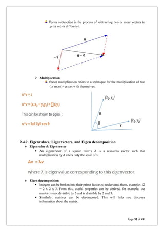
![2.4.3. Introduction to Calculus
Calculus is the study of change. It provides a framework for modelling systems in which there
is change and ways to make predictions of such models.
❖ Differential Calculus
✓ Differential calculus is a part of calculus that deals with the study of the rates at
which quantities change.
✓ Let x and y be two real numbers such that y is a function of x, that is, y = f(x).
✓ If f(x) is the equation of a straight line (linear equation), then the equation is
represented as y = mx + b.
✓ Where m is the slope determined by the following equation:
❖ Integral Calculus
✓ Integral Calculus assigns numbers to functions to describe displacement, area,
volume, and other concepts that arise by combining infinitesimal data.
✓ Given a function f of a real variable x and an interval [a, b] of the real line, the
definite integral is defined informally as the signed area of the region in the
xyplane that is bounded by the graph of f, the x -axis, and the vertical lines x=a
and x=b.
Page 32 of 49](https://image.slidesharecdn.com/intern-241223143925-cd1440a3/85/A-internship-report-on-artificial-intelligence-31-320.jpg)


![ARTIFICIAL INTILLIGENCE
An Internship Report
By
A. Geetha saranya(22JG5A0201)
Under the esteemed guidance of
Mr. Y. Ramu
Assistant Professor
EEE Department
Department of Electricals and Electronics Engineering
GAYATRIVIDYA PARISHAD COLLEGE OF ENGINEERING FOR WOMEN
[Approved by AICTE NEW DELHI, Affiliated to JNTUK Kakinada]
[Accredited by National Board of Accreditation for B.Tech. CSE, ECE & IT- Valid from 2019-22 2022-2025]
[Accredited by National Assessment and Accreditation Council (NAAC)– Valid from 2022-2027]
Komadi, MadhuraWada, Visakhapatnam–530048
2023-2024
GAYATRI VIDYA PARISHAD COLLEGE OF ENGINEERING FOR WOMEN](https://image.slidesharecdn.com/intern-241223143925-cd1440a3/75/A-internship-report-on-artificial-intelligence-1-2048.jpg)


![2.4.3. Introduction to Calculus
Calculus is the study of change. It provides a framework for modelling systems in which there
is change and ways to make predictions of such models.
❖ Differential Calculus
✓ Differential calculus is a part of calculus that deals with the study of the rates at
which quantities change.
✓ Let x and y be two real numbers such that y is a function of x, that is, y = f(x).
✓ If f(x) is the equation of a straight line (linear equation), then the equation is
represented as y = mx + b.
✓ Where m is the slope determined by the following equation:
❖ Integral Calculus
✓ Integral Calculus assigns numbers to functions to describe displacement, area,
volume, and other concepts that arise by combining infinitesimal data.
✓ Given a function f of a real variable x and an interval [a, b] of the real line, the
definite integral is defined informally as the signed area of the region in the
xyplane that is bounded by the graph of f, the x -axis, and the vertical lines x=a
and x=b.
Page 32 of 49](https://image.slidesharecdn.com/intern-241223143925-cd1440a3/75/A-internship-report-on-artificial-intelligence-31-2048.jpg)