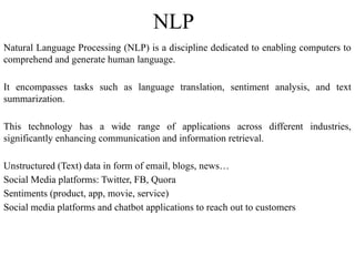
NLP
Natural Language Processing(NLP) is a discipline dedicated to enabling computers to
comprehend and generate human language.
It encompasses tasks such as language translation, sentiment analysis, and text
summarization.
This technology has a wide range of applications across different industries,
significantly enhancing communication and information retrieval.
Unstructured (Text) data in form of email, blogs, news…
Social Media platforms: Twitter, FB, Quora
Sentiments (product, app, movie, service)
Social media platforms and chatbot applications to reach out to customers
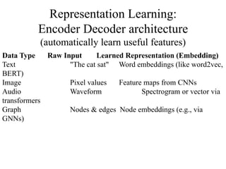
Representation Learning:
Encoder Decoderarchitecture
(automatically learn useful features)
Data Type Raw Input Learned Representation (Embedding)
Text "The cat sat" Word embeddings (like word2vec,
BERT)
Image Pixel values Feature maps from CNNs
Audio Waveform Spectrogram or vector via
transformers
Graph Nodes & edges Node embeddings (e.g., via
GNNs)
6.
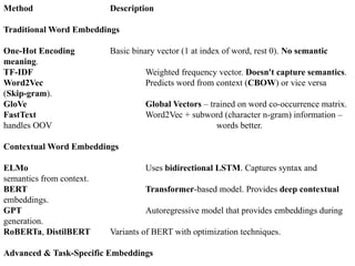
Method Description
Traditional WordEmbeddings
One-Hot Encoding Basic binary vector (1 at index of word, rest 0). No semantic
meaning.
TF-IDF Weighted frequency vector. Doesn't capture semantics.
Word2Vec Predicts word from context (CBOW) or vice versa
(Skip-gram).
GloVe Global Vectors – trained on word co-occurrence matrix.
FastText Word2Vec + subword (character n-gram) information –
handles OOV words better.
Contextual Word Embeddings
ELMo Uses bidirectional LSTM. Captures syntax and
semantics from context.
BERT Transformer-based model. Provides deep contextual
embeddings.
GPT Autoregressive model that provides embeddings during
generation.
RoBERTa, DistilBERT Variants of BERT with optimization techniques.
Advanced & Task-Specific Embeddings
7.
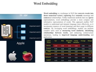
Word Embedding
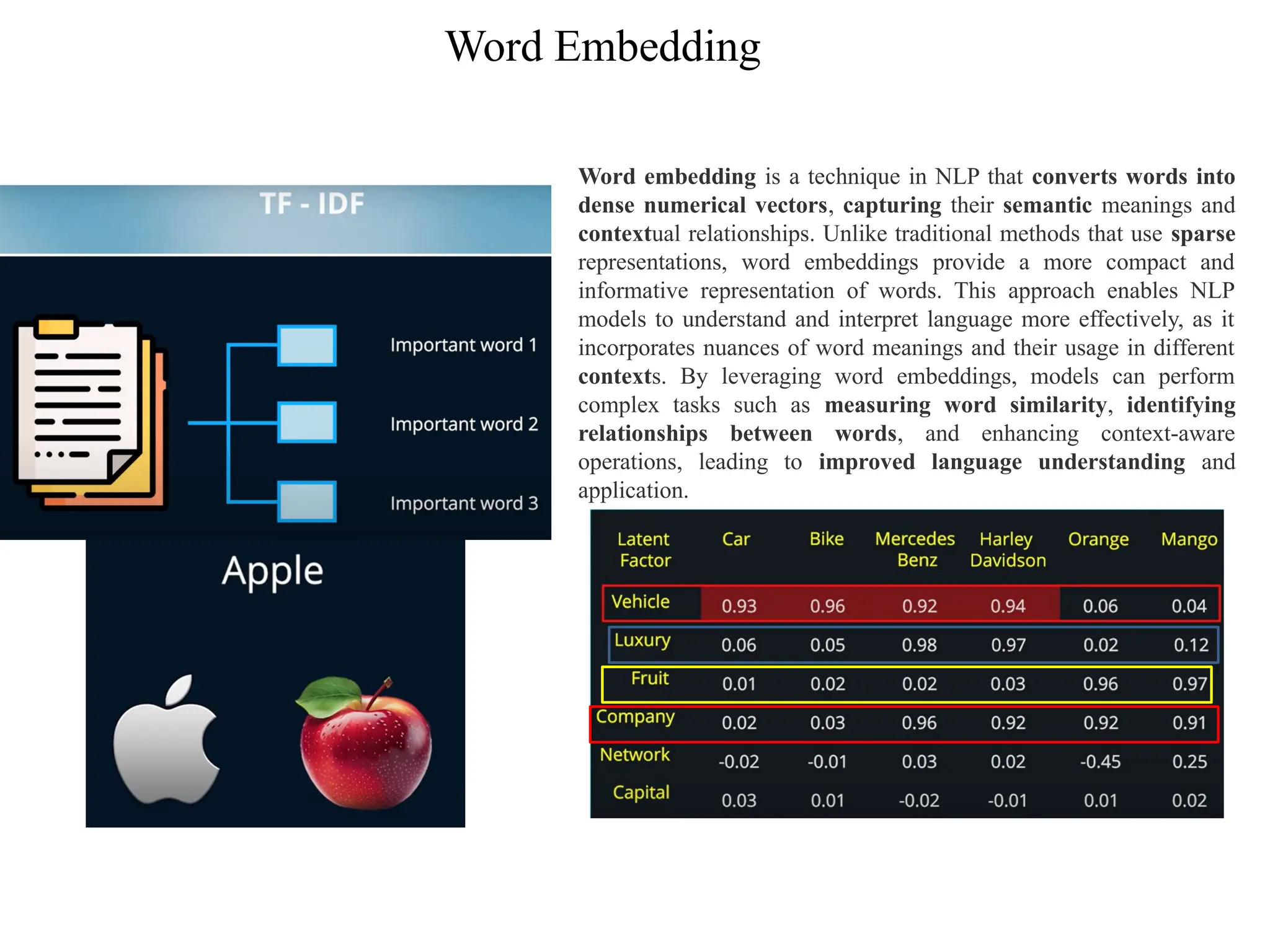
Word embeddingis a technique in NLP that converts words into
dense numerical vectors, capturing their semantic meanings and
contextual relationships. Unlike traditional methods that use sparse
representations, word embeddings provide a more compact and
informative representation of words. This approach enables NLP
models to understand and interpret language more effectively, as it
incorporates nuances of word meanings and their usage in different
contexts. By leveraging word embeddings, models can perform
complex tasks such as measuring word similarity, identifying
relationships between words, and enhancing context-aware
operations, leading to improved language understanding and
application.
8.
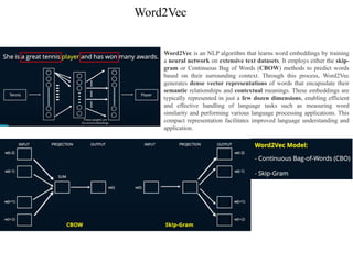
Word2Vec
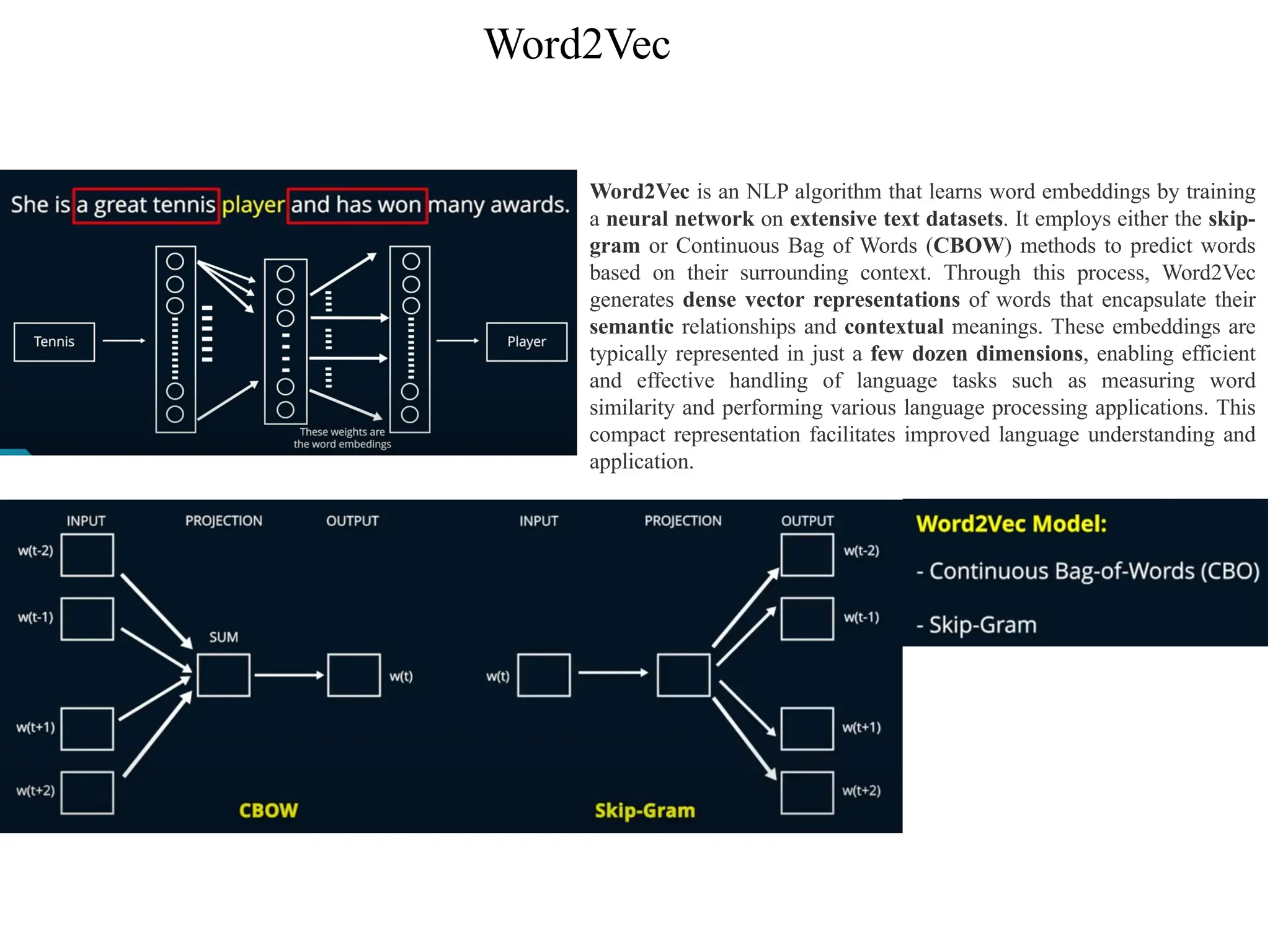
Word2Vec is anNLP algorithm that learns word embeddings by training
a neural network on extensive text datasets. It employs either the skip-
gram or Continuous Bag of Words (CBOW) methods to predict words
based on their surrounding context. Through this process, Word2Vec
generates dense vector representations of words that encapsulate their
semantic relationships and contextual meanings. These embeddings are
typically represented in just a few dozen dimensions, enabling efficient
and effective handling of language tasks such as measuring word
similarity and performing various language processing applications. This
compact representation facilitates improved language understanding and
application.
9.
from gensim.models importWord2Vec
# Sample corpus
corpus = [["I", "love", "this", "movie"],
["This", "movie", "is", "terrible"],
["The", "plot", "is", "confusing"]]
# Skip-gram model
model = Word2Vec(sentences=corpus, min_count=1, sg=1)
# Print word vectors
for word in model.wv.key_to_index:
print(word, model.wv.get_vector(word))
# CBOW model
model = Word2Vec(sentences=corpus, min_count=1, sg=0)
# Print word vectors
for word in model.wv.key_to_index:
print(word, model.wv.get_vector(word))
i [ 0.0156 0.0331 -0.0394 ... 0.0742]
love [-0.0173 0.0469 0.0128 ... 0.0883]
this [ 0.0322 -0.0254 -0.0016 ... 0.0594]
i [-0.0021 0.0511 -0.0423 ... 0.0147]
love [ 0.0144 -0.0389 0.0290 ... 0.0231]
this [-0.0216 0.0374 0.0057 ... -0.0129]
10.
Word Embedding
GloVe –Global Vectors for word representation
The model is trained on multiple data sets including
Wikipedia, Twitter and Common Crawl on billions of
tokens and the embeddings are represented in
different dimension size ranging from 50 to 300.
“glove.6B.zip” file
consider the 50-dimension representation
use the dimension reduction technique like t-SNE
that is, t-Distributed Stochastic Neighbor embedding
to reduce the dimensions to 2 and plot around 500
words on those 2-dimensions
import gensim.downloader as api
glove_model = api.load('glove-twitter-25')
sample_glove_embedding=glove_model['computer'];
12.
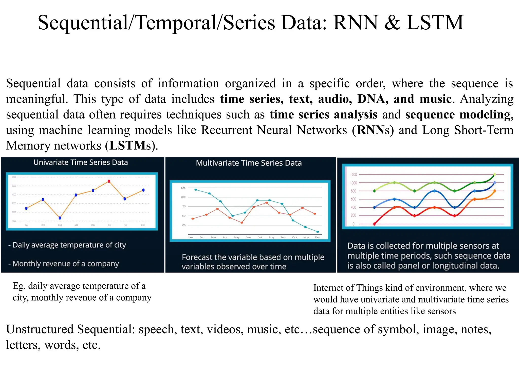
Sequential/Temporal/Series Data: RNN& LSTM
Sequential data consists of information organized in a specific order, where the sequence is
meaningful. This type of data includes time series, text, audio, DNA, and music. Analyzing
sequential data often requires techniques such as time series analysis and sequence modeling,
using machine learning models like Recurrent Neural Networks (RNNs) and Long Short-Term
Memory networks (LSTMs).
Unstructured Sequential: speech, text, videos, music, etc…sequence of symbol, image, notes,
letters, words, etc.
Eg. daily average temperature of a
city, monthly revenue of a company
Internet of Things kind of environment, where we
would have univariate and multivariate time series
data for multiple entities like sensors
13.
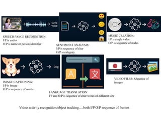
SPEECH/VOICE RECOGNITION:
I/P isaudio
O/P is name or person identifier SENTIMENT ANALYSIS:
I/P is sequence of char
O/P is category
MUSIC CREATION:
I/P is single value
O/P is sequence of nodes
IMAGE CAPTIONING:
I/P is image
O/P is sequence of words
LANGUAGE TRANSLATION:
I/P and O/P is sequence of char/words of different size
VIDEO FILES: Sequence of
images
Video activity recognition/object tracking….both I/P O/P sequence of frames
14.
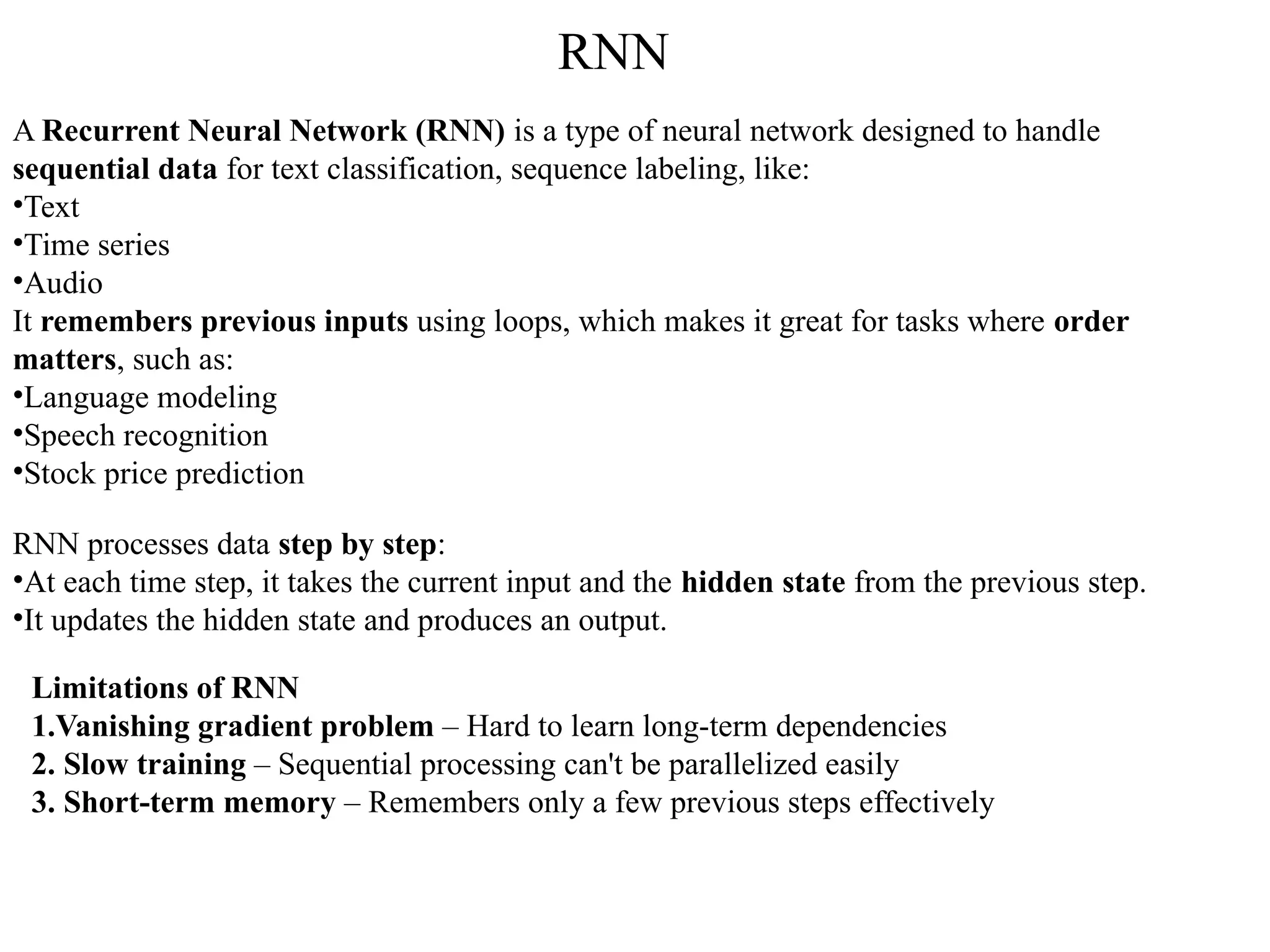
A Recurrent NeuralNetwork (RNN) is a type of neural network designed to handle
sequential data for text classification, sequence labeling, like:
•Text
•Time series
•Audio
It remembers previous inputs using loops, which makes it great for tasks where order
matters, such as:
•Language modeling
•Speech recognition
•Stock price prediction
RNN processes data step by step:
•At each time step, it takes the current input and the hidden state from the previous step.
•It updates the hidden state and produces an output.
Limitations of RNN
1.Vanishing gradient problem – Hard to learn long-term dependencies
2. Slow training – Sequential processing can't be parallelized easily
3. Short-term memory – Remembers only a few previous steps effectively
RNN
15.
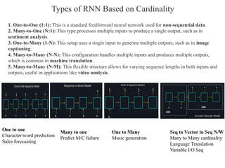
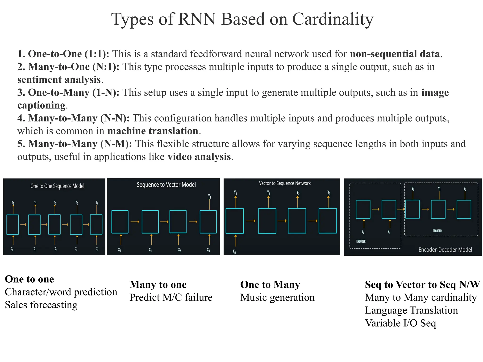
Types of RNNBased on Cardinality
1. One-to-One (1:1): This is a standard feedforward neural network used for non-sequential data.
2. Many-to-One (N:1): This type processes multiple inputs to produce a single output, such as in
sentiment analysis.
3. One-to-Many (1-N): This setup uses a single input to generate multiple outputs, such as in image
captioning.
4. Many-to-Many (N-N): This configuration handles multiple inputs and produces multiple outputs,
which is common in machine translation.
5. Many-to-Many (N-M): This flexible structure allows for varying sequence lengths in both inputs and
outputs, useful in applications like video analysis.
One to one
Character/word prediction
Sales forecasting
Many to one
Predict M/C failure
One to Many
Music generation
Seq to Vector to Seq N/W
Many to Many cardinality
Language Translation
Variable I/O Seq
16.
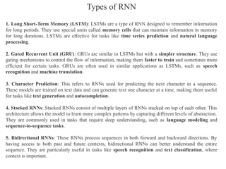
1. Long Short-TermMemory (LSTM): LSTMs are a type of RNN designed to remember information
for long periods. They use special units called memory cells that can maintain information in memory
for long durations. LSTMs are effective for tasks like time series prediction and natural language
processing.
2. Gated Recurrent Unit (GRU): GRUs are similar to LSTMs but with a simpler structure. They use
gating mechanisms to control the flow of information, making them faster to train and sometimes more
efficient for certain tasks. GRUs are often used in similar applications as LSTMs, such as speech
recognition and machine translation.
3. Character Prediction: This refers to RNNs used for predicting the next character in a sequence.
These models are trained on text data and can generate text one character at a time, making them useful
for tasks like text generation and autocompletion.
4. Stacked RNNs: Stacked RNNs consist of multiple layers of RNNs stacked on top of each other. This
architecture allows the model to learn more complex patterns by capturing different levels of abstraction.
They are commonly used in tasks that require deep understanding, such as language modeling and
sequence-to-sequence tasks.
5. Bidirectional RNNs: These RNNs process sequences in both forward and backward directions. By
having access to both past and future contexts, bidirectional RNNs can better understand the entire
sequence. They are particularly useful in tasks like speech recognition and text classification, where
context is important.
Types of RNN
18.
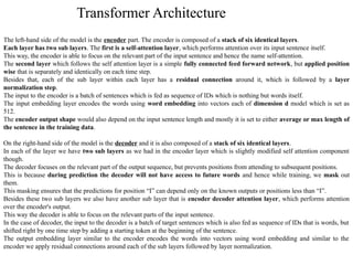
The left-hand sideof the model is the encoder part. The encoder is composed of a stack of six identical layers.
Each layer has two sub layers. The first is a self-attention layer, which performs attention over its input sentence itself.
This way, the encoder is able to focus on the relevant part of the input sentence and hence the name self-attention.
The second layer which follows the self attention layer is a simple fully connected feed forward network, but applied position
wise that is separately and identically on each time step.
Besides that, each of the sub layer within each layer has a residual connection around it, which is followed by a layer
normalization step.
The input to the encoder is a batch of sentences which is fed as sequence of IDs which is nothing but words itself.
The input embedding layer encodes the words using word embedding into vectors each of dimension d model which is set as
512.
The encoder output shape would also depend on the input sentence length and mostly it is set to either average or max length of
the sentence in the training data.
On the right-hand side of the model is the decoder and it is also composed of a stack of six identical layers.
In each of the layer we have two sub layers as we had in the encoder layer which is slightly modified self attention component
though.
The decoder focuses on the relevant part of the output sequence, but prevents positions from attending to subsequent positions.
This is because during prediction the decoder will not have access to future words and hence while training, we mask out
them.
This masking ensures that the predictions for position “I” can depend only on the known outputs or positions less than “I”.
Besides these two sub layers we also have another sub layer that is encoder decoder attention layer, which performs attention
over the encoder's output.
This way the decoder is able to focus on the relevant parts of the input sentence.
In the case of decoder, the input to the decoder is a batch of target sentences which is also fed as sequence of IDs that is words, but
shifted right by one time step by adding a starting token at the beginning of the sentence.
The output embedding layer similar to the encoder encodes the words into vectors using word embedding and similar to the
encoder we apply residual connections around each of the sub layers followed by layer normalization.
Transformer Architecture
19.
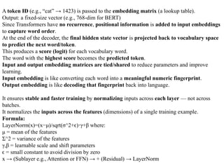
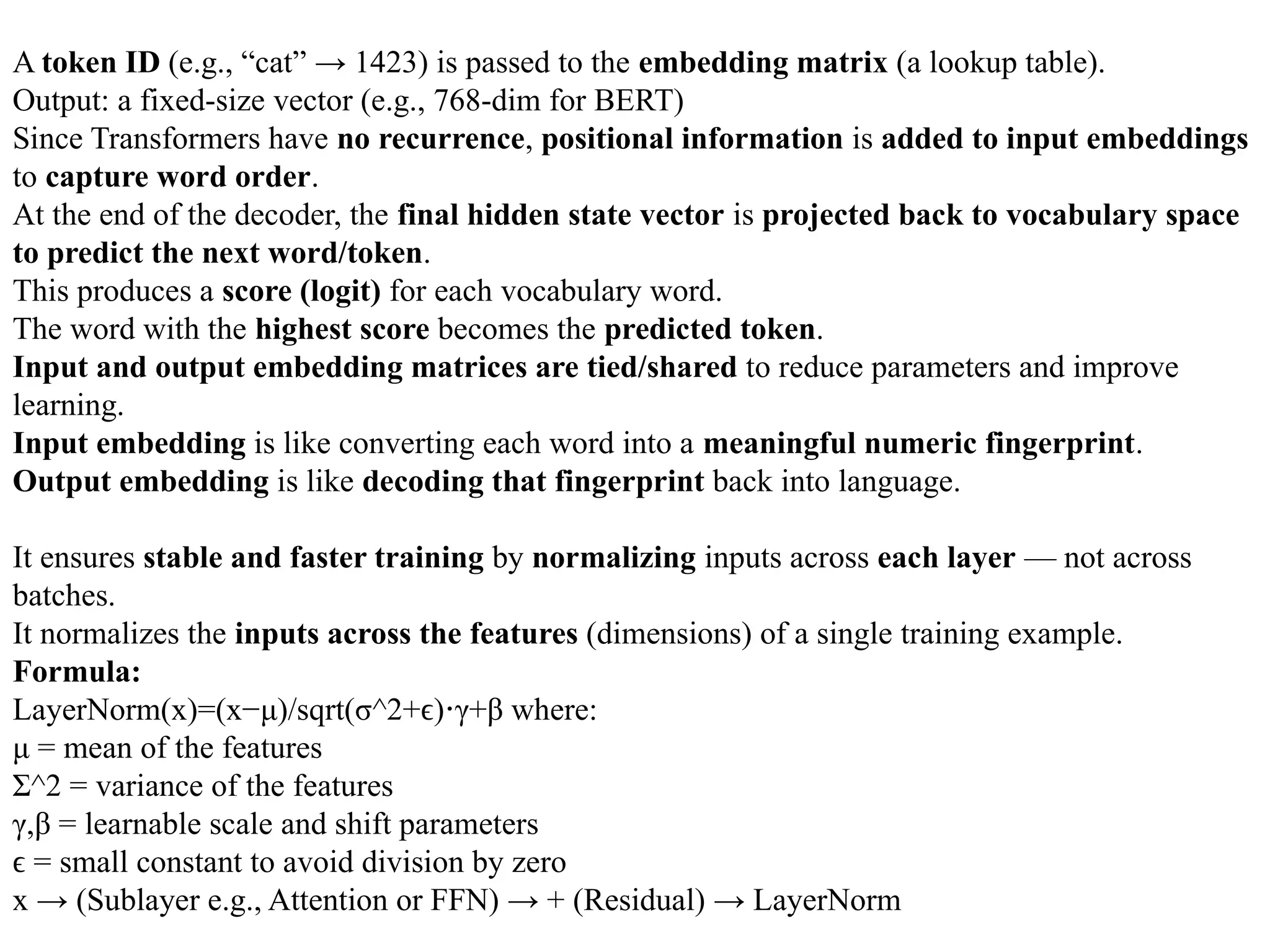
A token ID(e.g., “cat” → 1423) is passed to the embedding matrix (a lookup table).
Output: a fixed-size vector (e.g., 768-dim for BERT)
Since Transformers have no recurrence, positional information is added to input embeddings
to capture word order.
At the end of the decoder, the final hidden state vector is projected back to vocabulary space
to predict the next word/token.
This produces a score (logit) for each vocabulary word.
The word with the highest score becomes the predicted token.
Input and output embedding matrices are tied/shared to reduce parameters and improve
learning.
Input embedding is like converting each word into a meaningful numeric fingerprint.
Output embedding is like decoding that fingerprint back into language.
It ensures stable and faster training by normalizing inputs across each layer — not across
batches.
It normalizes the inputs across the features (dimensions) of a single training example.
Formula:
LayerNorm(x)=(x−μ)/sqrt(σ^2+ϵ) γ+β
⋅ where:
μ = mean of the features
Σ^2 = variance of the features
γ,β = learnable scale and shift parameters
=
ϵ small constant to avoid division by zero
x → (Sublayer e.g., Attention or FFN) → + (Residual) → LayerNorm
20.
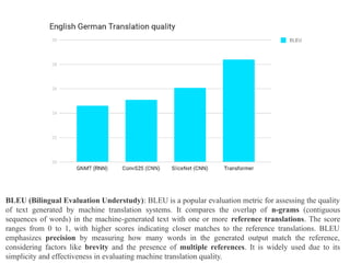
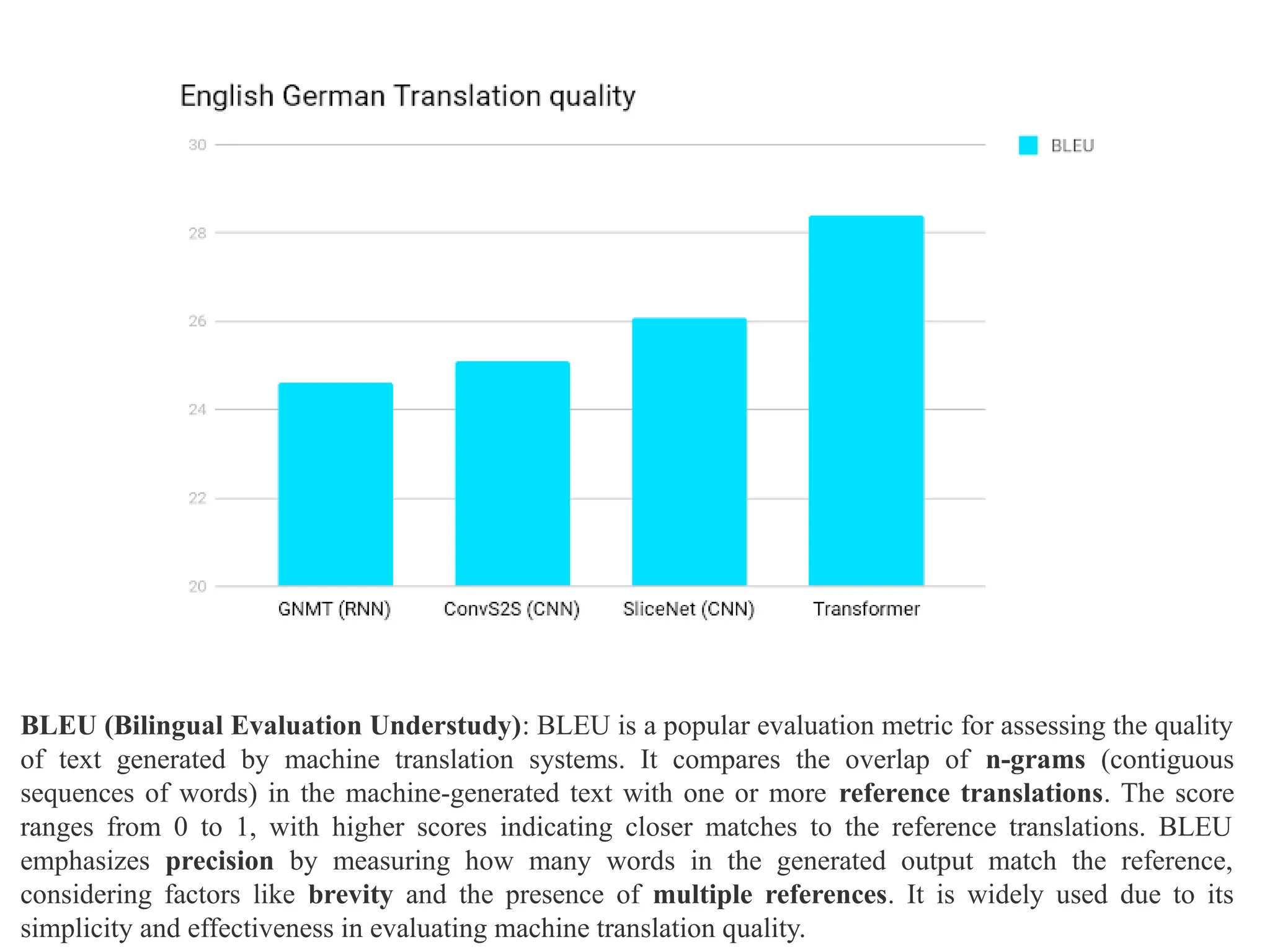
BLEU (Bilingual EvaluationUnderstudy): BLEU is a popular evaluation metric for assessing the quality
of text generated by machine translation systems. It compares the overlap of n-grams (contiguous
sequences of words) in the machine-generated text with one or more reference translations. The score
ranges from 0 to 1, with higher scores indicating closer matches to the reference translations. BLEU
emphasizes precision by measuring how many words in the generated output match the reference,
considering factors like brevity and the presence of multiple references. It is widely used due to its
simplicity and effectiveness in evaluating machine translation quality.
21.
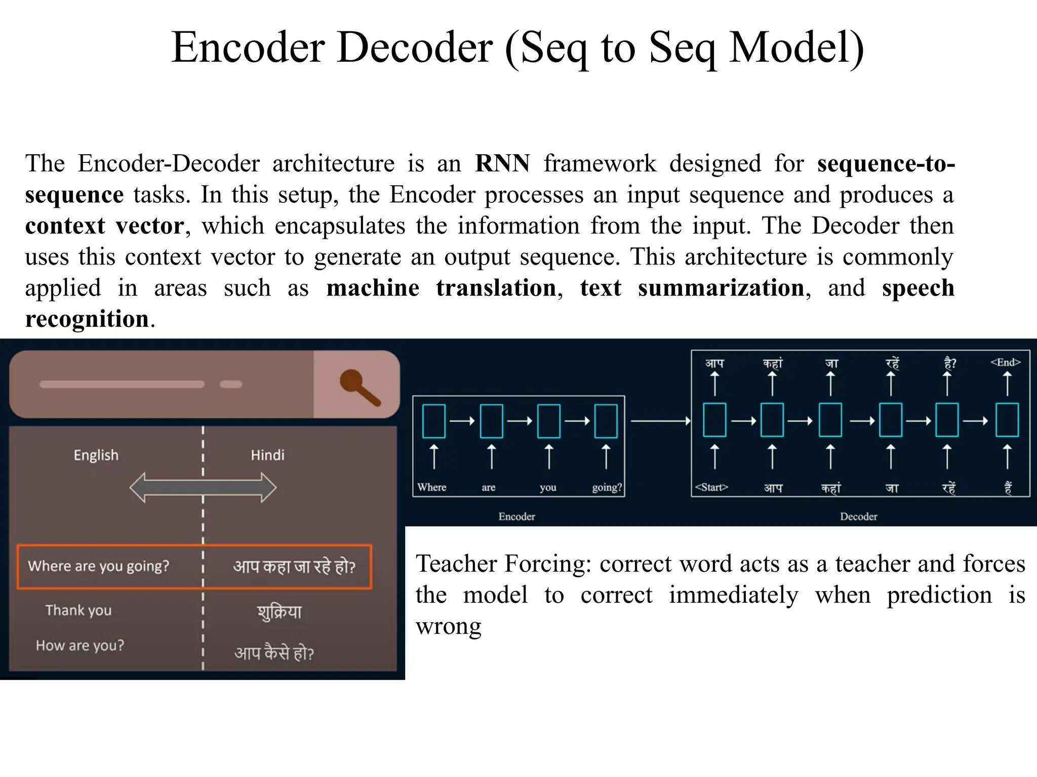
Encoder Decoder (Seqto Seq Model)
The Encoder-Decoder architecture is an RNN framework designed for sequence-to-
sequence tasks. In this setup, the Encoder processes an input sequence and produces a
context vector, which encapsulates the information from the input. The Decoder then
uses this context vector to generate an output sequence. This architecture is commonly
applied in areas such as machine translation, text summarization, and speech
recognition.
Teacher Forcing: correct word acts as a teacher and forces
the model to correct immediately when prediction is
wrong
22.
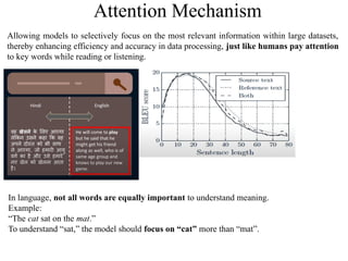
Attention Mechanism
Allowing modelsto selectively focus on the most relevant information within large datasets,
thereby enhancing efficiency and accuracy in data processing, just like humans pay attention
to key words while reading or listening.
In language, not all words are equally important to understand meaning.
Example:
“The cat sat on the mat.”
To understand “sat,” the model should focus on “cat” more than “mat”.
23.
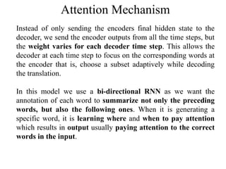
Instead of onlysending the encoders final hidden state to the
decoder, we send the encoder outputs from all the time steps, but
the weight varies for each decoder time step. This allows the
decoder at each time step to focus on the corresponding words at
the encoder that is, choose a subset adaptively while decoding
the translation.
In this model we use a bi-directional RNN as we want the
annotation of each word to summarize not only the preceding
words, but also the following ones. When it is generating a
specific word, it is learning where and when to pay attention
which results in output usually paying attention to the correct
words in the input.
Attention Mechanism
24.
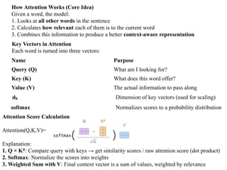
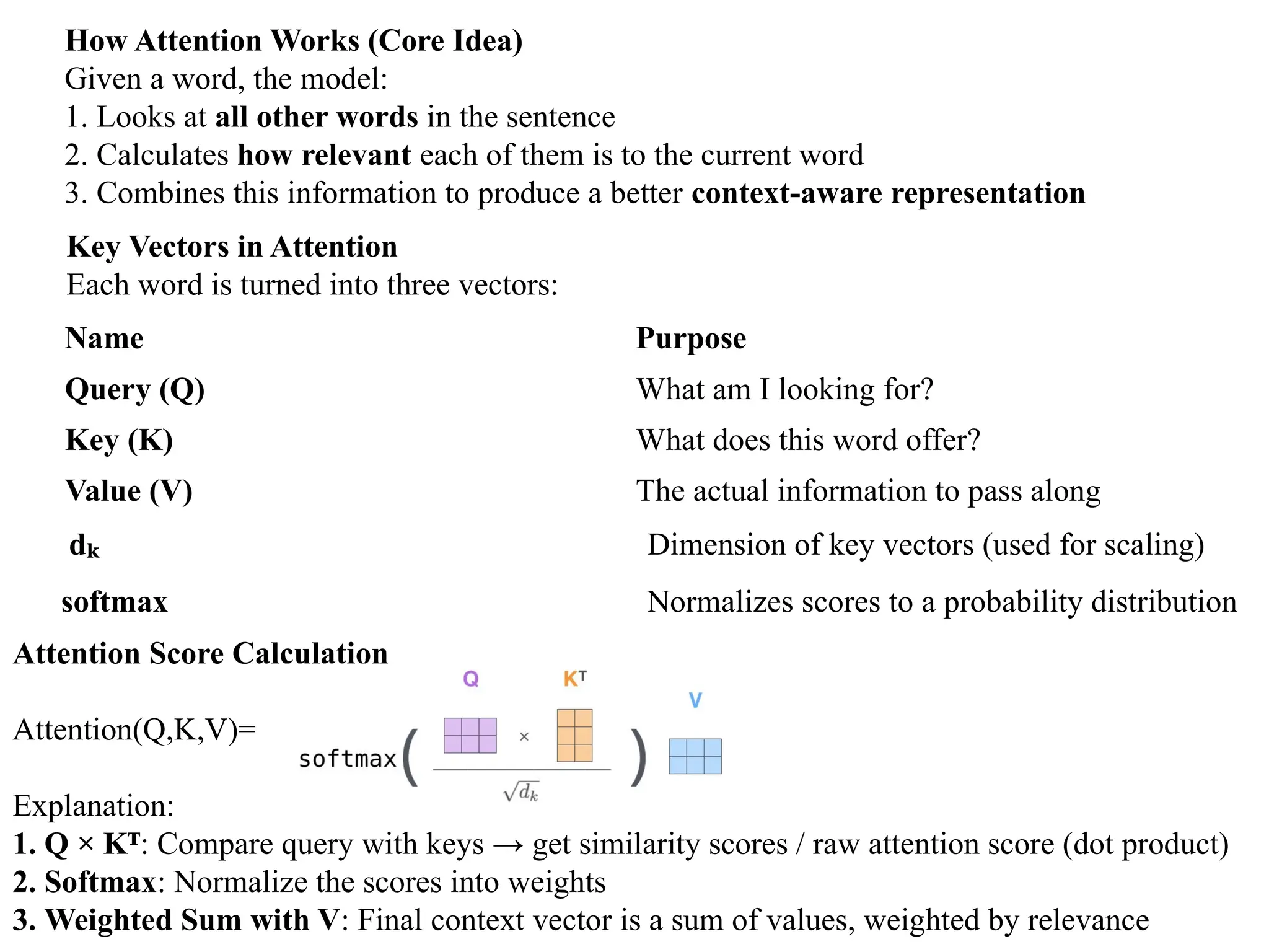
How Attention Works(Core Idea)
Given a word, the model:
1. Looks at all other words in the sentence
2. Calculates how relevant each of them is to the current word
3. Combines this information to produce a better context-aware representation
Name Purpose
Query (Q) What am I looking for?
Key (K) What does this word offer?
Value (V) The actual information to pass along
Key Vectors in Attention
Each word is turned into three vectors:
Attention Score Calculation
Attention(Q,K,V)=
Explanation:
1. Q × Kᵀ: Compare query with keys → get similarity scores / raw attention score (dot product)
2. Softmax: Normalize the scores into weights
3. Weighted Sum with V: Final context vector is a sum of values, weighted by relevance
dₖ Dimension of key vectors (used for scaling)
softmax Normalizes scores to a probability distribution
25.
import tensorflow astf
from tensorflow.keras.layers import Layer
class ScaledDotProductAttention(Layer):
def __init__(self):
super(ScaledDotProductAttention, self).__init__()
def call(self, query, key, value, mask=None):
# Step 1: Calculate dot product (QK )
ᵀ
matmul_qk = tf.matmul(query, key, transpose_b=True)
# Step 2: Scale the dot product by sqrt(d_k)
dk = tf.cast(tf.shape(key)[-1], tf.float32) # key dimension
scaled_attention_logits = matmul_qk / tf.math.sqrt(dk)
# Step 3: Apply mask (optional, for padding or future words)
if mask is not None:
scaled_attention_logits += (mask * -1e9) # very negative to nullify softmax
# Step 4: Softmax to get attention weights
attention_weights = tf.nn.softmax(scaled_attention_logits, axis=-1)
# Step 5: Multiply by V (weighted sum of values)
output = tf.matmul(attention_weights, value)
return output, attention_weights
Scaled dot product attention
26.
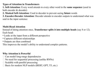
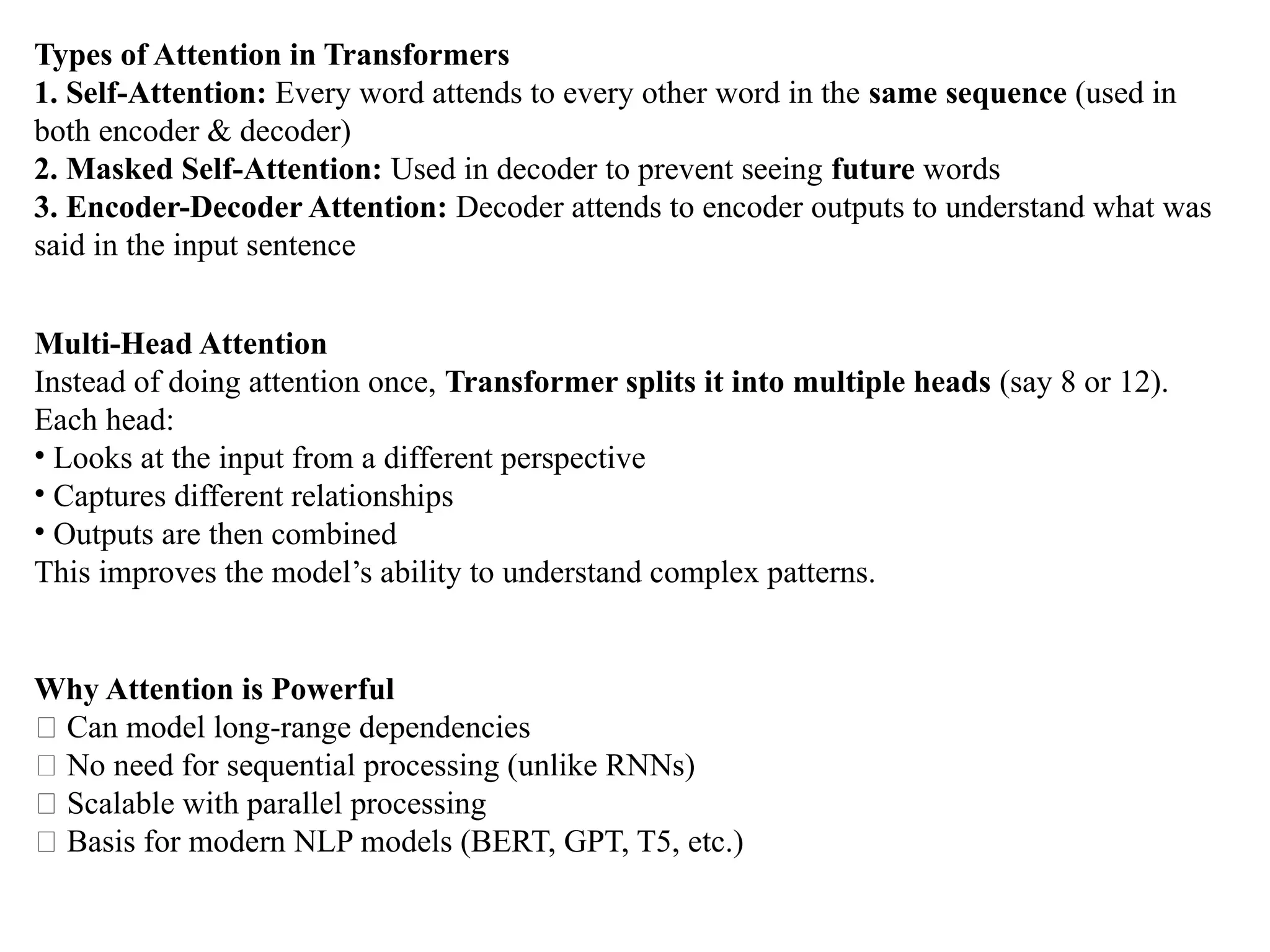
Types of Attentionin Transformers
1. Self-Attention: Every word attends to every other word in the same sequence (used in
both encoder & decoder)
2. Masked Self-Attention: Used in decoder to prevent seeing future words
3. Encoder-Decoder Attention: Decoder attends to encoder outputs to understand what was
said in the input sentence
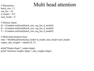
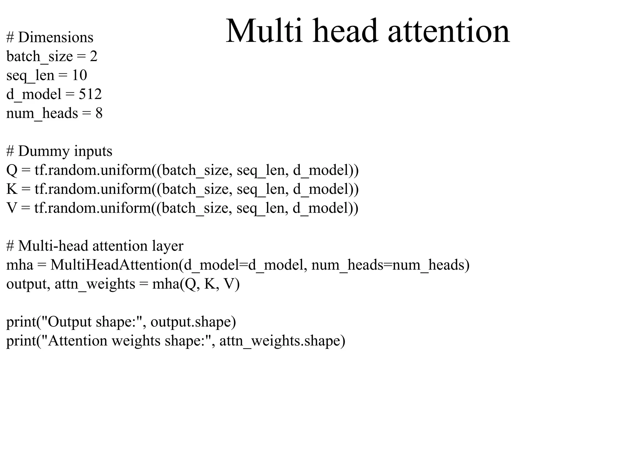
Multi-Head Attention
Instead of doing attention once, Transformer splits it into multiple heads (say 8 or 12).
Each head:
• Looks at the input from a different perspective
• Captures different relationships
• Outputs are then combined
This improves the model’s ability to understand complex patterns.
Why Attention is Powerful
✅ Can model long-range dependencies
✅ No need for sequential processing (unlike RNNs)
✅ Scalable with parallel processing
✅ Basis for modern NLP models (BERT, GPT, T5, etc.)
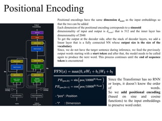
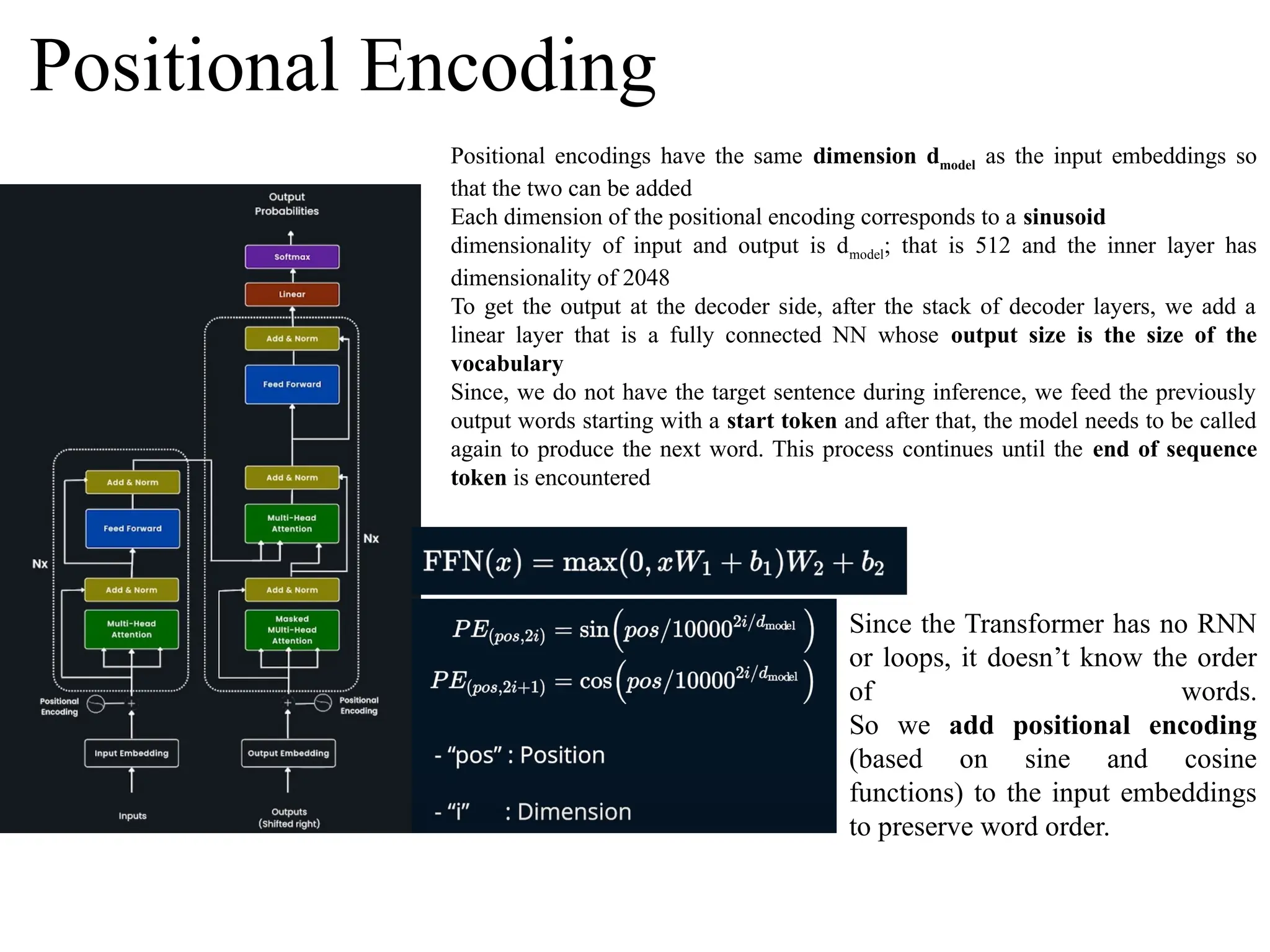
Positional Encoding
Positional encodingshave the same dimension dmodel as the input embeddings so
that the two can be added
Each dimension of the positional encoding corresponds to a sinusoid
dimensionality of input and output is dmodel; that is 512 and the inner layer has
dimensionality of 2048
To get the output at the decoder side, after the stack of decoder layers, we add a
linear layer that is a fully connected NN whose output size is the size of the
vocabulary
Since, we do not have the target sentence during inference, we feed the previously
output words starting with a start token and after that, the model needs to be called
again to produce the next word. This process continues until the end of sequence
token is encountered
Since the Transformer has no RNN
or loops, it doesn’t know the order
of words.
So we add positional encoding
(based on sine and cosine
functions) to the input embeddings
to preserve word order.
30.
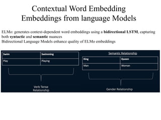
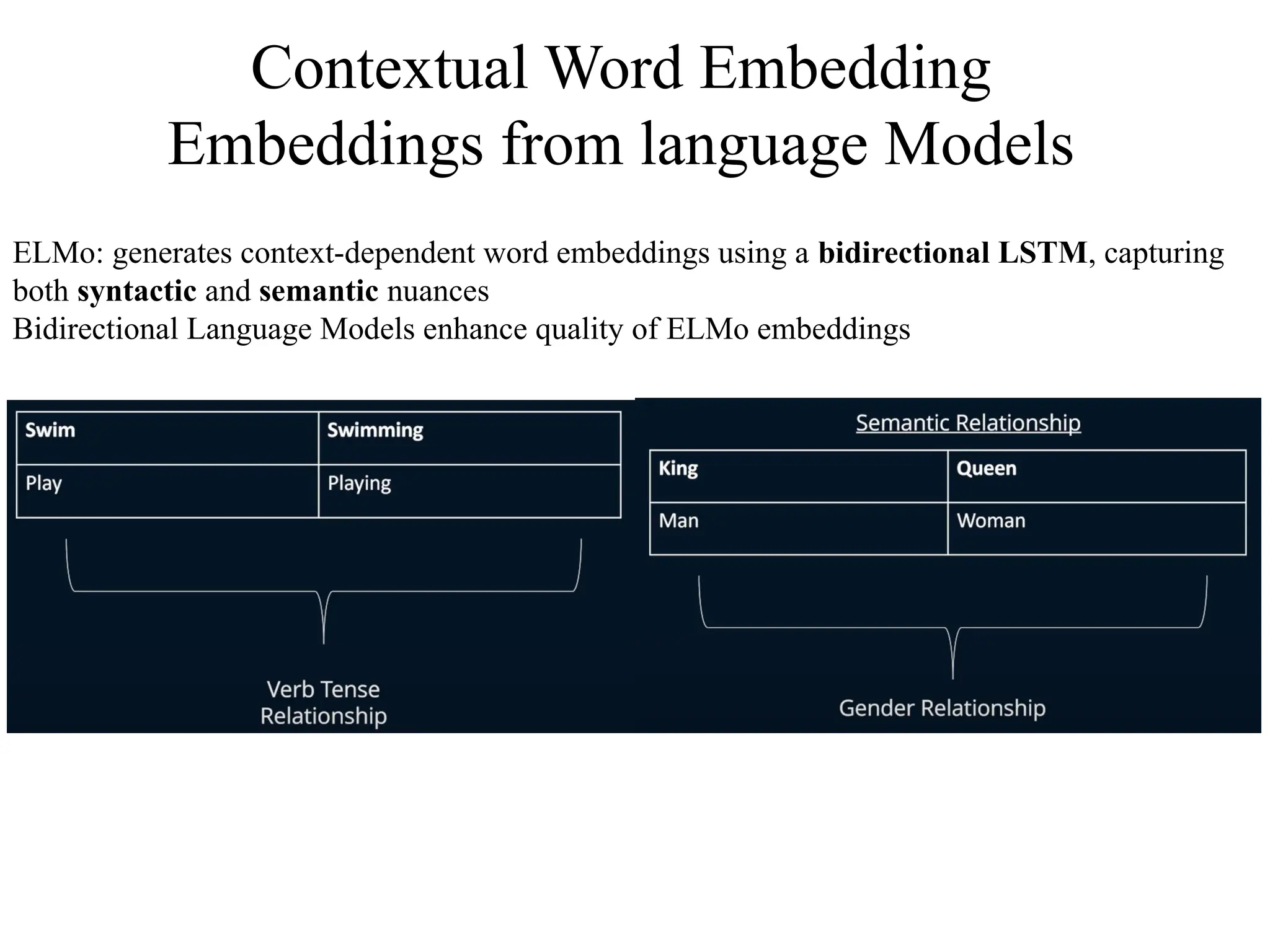
Contextual Word Embedding
Embeddingsfrom language Models
ELMo: generates context-dependent word embeddings using a bidirectional LSTM, capturing
both syntactic and semantic nuances
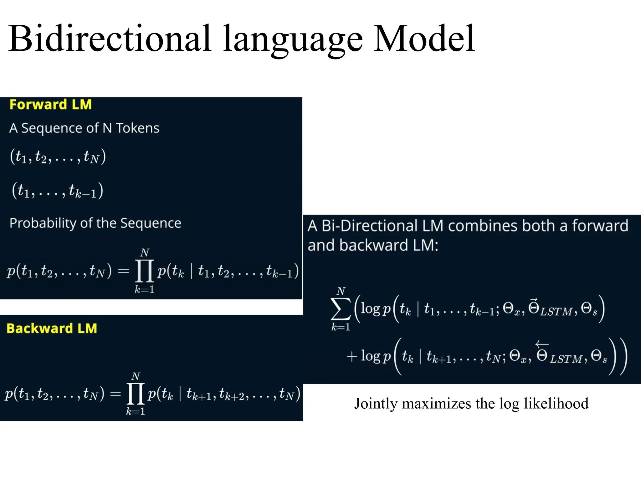
Bidirectional Language Models enhance quality of ELMo embeddings
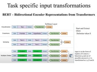
Task specific inputtransformations
Softmax Layer
BERT – Bidirectional Encoder Representations from Transformers
Start and Extract
token
Delimiter token $
input is in the form of
triplets of Context z
Question q and set of
possible answers k, it is
transformed as z q $ and k
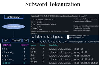
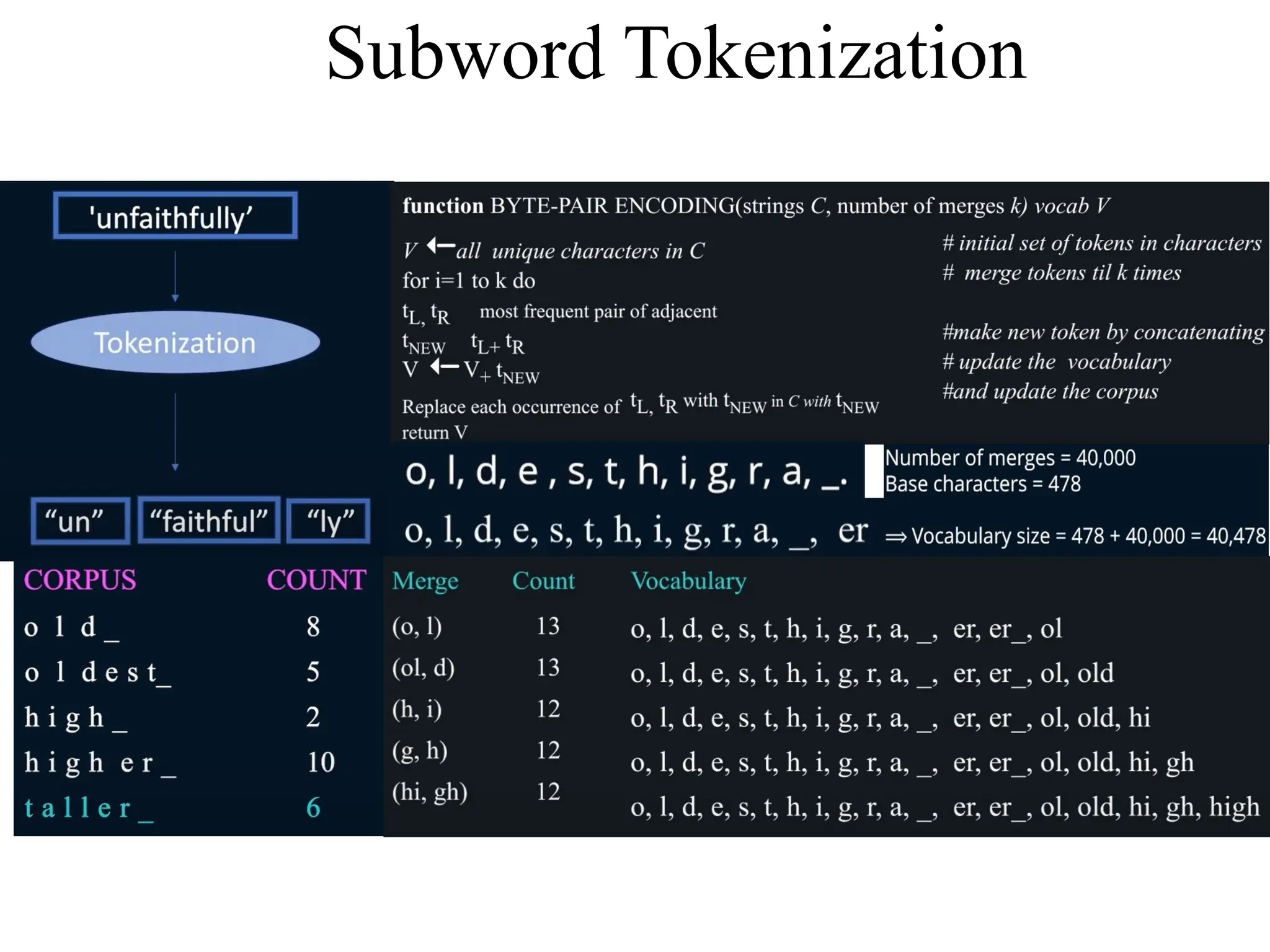
Initialize Vocabulary
Start witha vocabulary of all characters in the training text.
Tokenize Text as Characters
Example: "low", "lower" → ["l", "o", "w"], ["l", "o", "w", "e", "r"]
Count Pair Frequencies
Count all adjacent pairs of tokens.
Example: ("l", "o"), ("o", "w"), ("w", "e"), etc.
Merge Most Frequent Pair
Merge the pair with the highest frequency into a new symbol.
Example: If ("l", "o") is most frequent → replace it with "lo"
Repeat Steps 3–4
Continue merging the most frequent pairs until you reach a desired vocabulary size.
• Handles Out-of-Vocabulary (OOV) Words: Instead of treating unknown words as <unk>,
BPE breaks them into subword units.
• Reduces Vocabulary Size: Saves memory and speeds up training.
• Captures Morphological Structure: Helps models generalize better across similar words (e.g.,
"play", "playing", "played").
Byte Pair Encoding
35.
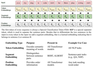
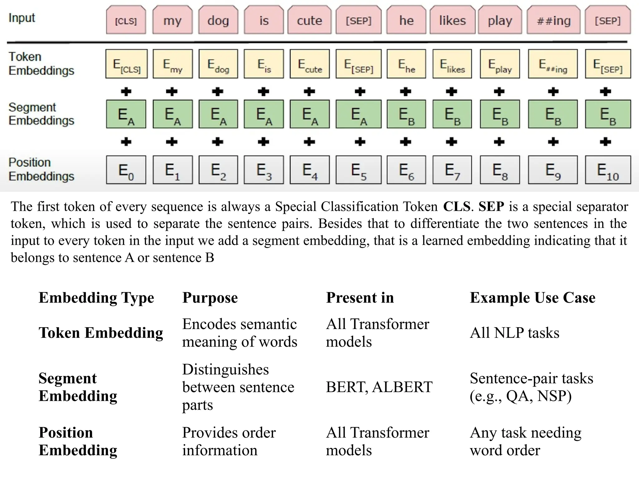
The first tokenof every sequence is always a Special Classification Token CLS. SEP is a special separator
token, which is used to separate the sentence pairs. Besides that to differentiate the two sentences in the
input to every token in the input we add a segment embedding, that is a learned embedding indicating that it
belongs to sentence A or sentence B
Embedding Type Purpose Present in Example Use Case
Token Embedding
Encodes semantic
meaning of words
All Transformer
models
All NLP tasks
Segment
Embedding
Distinguishes
between sentence
parts
BERT, ALBERT
Sentence-pair tasks
(e.g., QA, NSP)
Position
Embedding
Provides order
information
All Transformer
models
Any task needing
word order
37.
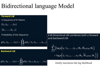
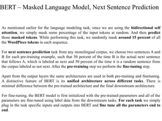
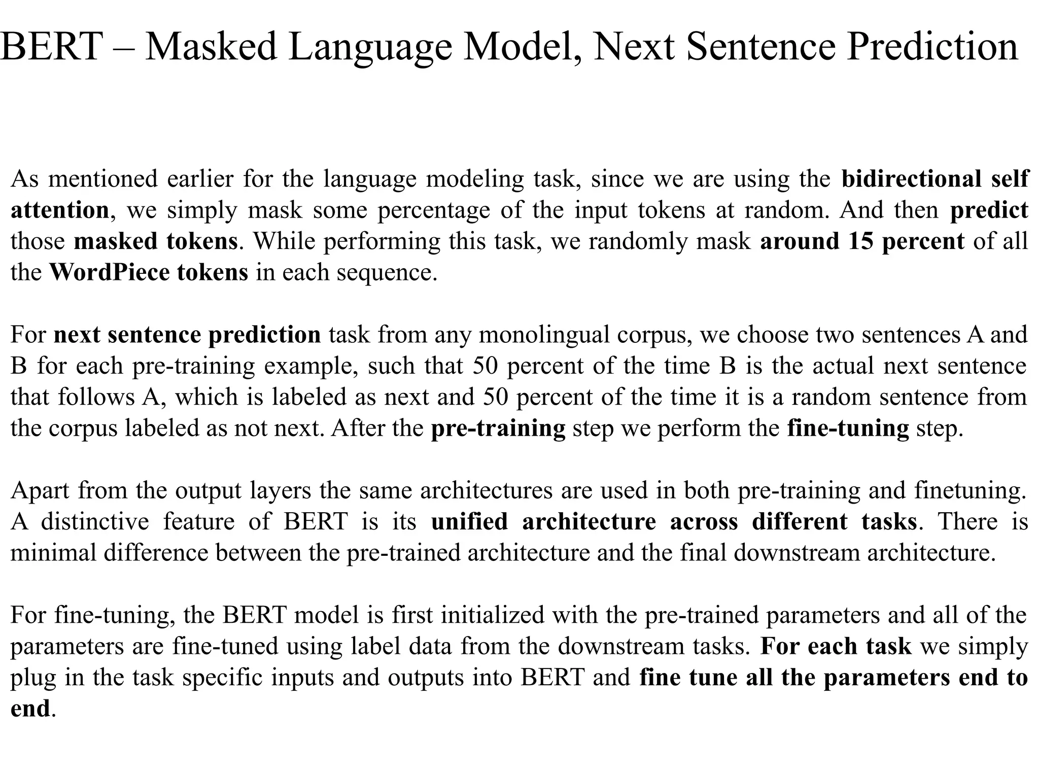
As mentioned earlierfor the language modeling task, since we are using the bidirectional self
attention, we simply mask some percentage of the input tokens at random. And then predict
those masked tokens. While performing this task, we randomly mask around 15 percent of all
the WordPiece tokens in each sequence.
For next sentence prediction task from any monolingual corpus, we choose two sentences A and
B for each pre-training example, such that 50 percent of the time B is the actual next sentence
that follows A, which is labeled as next and 50 percent of the time it is a random sentence from
the corpus labeled as not next. After the pre-training step we perform the fine-tuning step.
Apart from the output layers the same architectures are used in both pre-training and finetuning.
A distinctive feature of BERT is its unified architecture across different tasks. There is
minimal difference between the pre-trained architecture and the final downstream architecture.
For fine-tuning, the BERT model is first initialized with the pre-trained parameters and all of the
parameters are fine-tuned using label data from the downstream tasks. For each task we simply
plug in the task specific inputs and outputs into BERT and fine tune all the parameters end to
end.
BERT – Masked Language Model, Next Sentence Prediction
38.
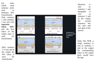
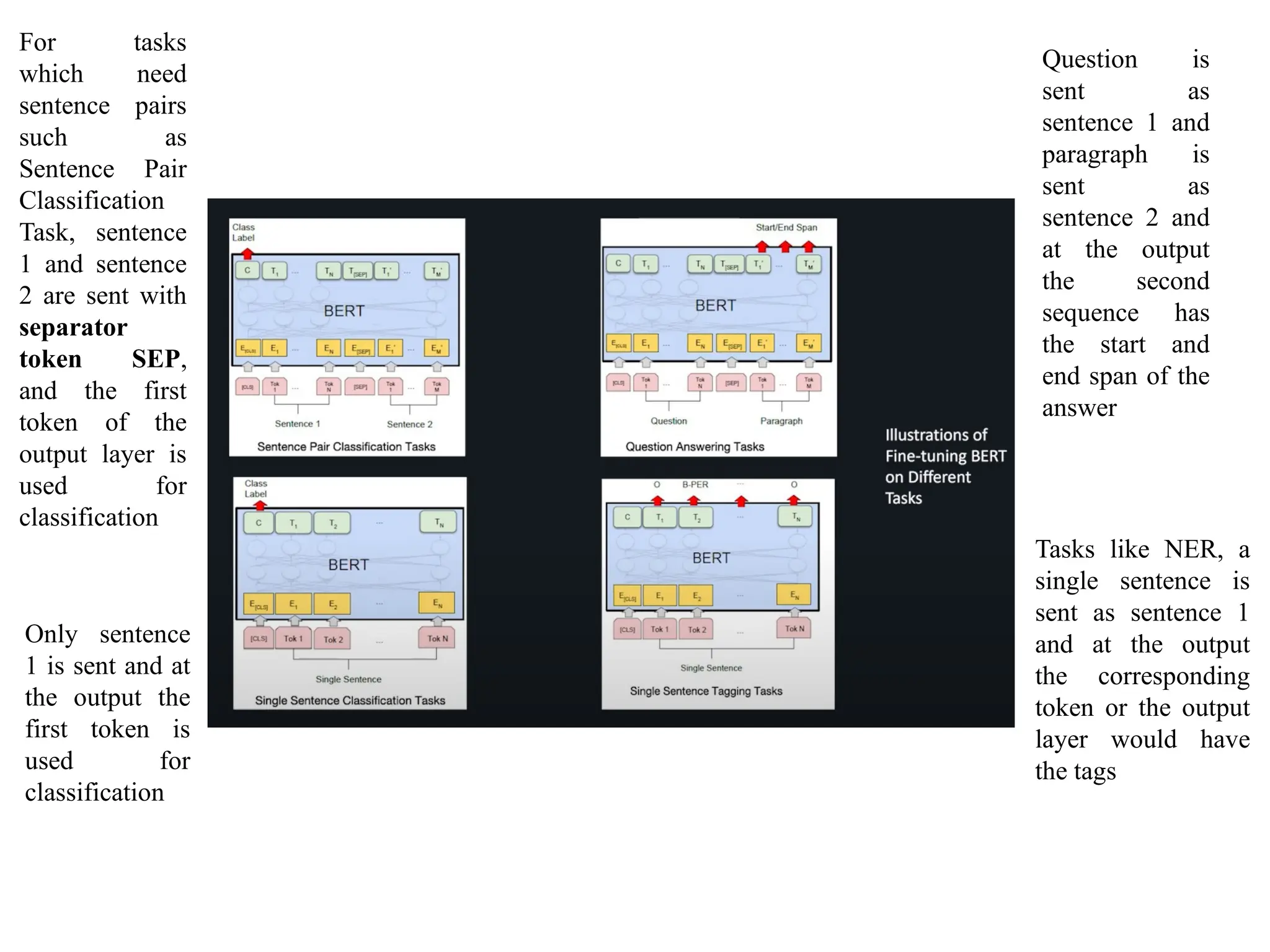
For tasks
which need
sentencepairs
such as
Sentence Pair
Classification
Task, sentence
1 and sentence
2 are sent with
separator
token SEP,
and the first
token of the
output layer is
used for
classification
Question is
sent as
sentence 1 and
paragraph is
sent as
sentence 2 and
at the output
the second
sequence has
the start and
end span of the
answer
Only sentence
1 is sent and at
the output the
first token is
used for
classification
Tasks like NER, a
single sentence is
sent as sentence 1
and at the output
the corresponding
token or the output
layer would have
the tags
39.
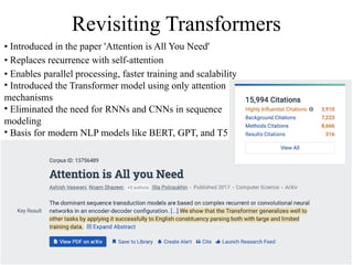
Revisiting Transformers
• Introducedin the paper 'Attention is All You Need'
• Replaces recurrence with self-attention
• Enables parallel processing, faster training and scalability
• Introduced the Transformer model using only attention
mechanisms
• Eliminated the need for RNNs and CNNs in sequence
modeling
• Basis for modern NLP models like BERT, GPT, and T5
40.
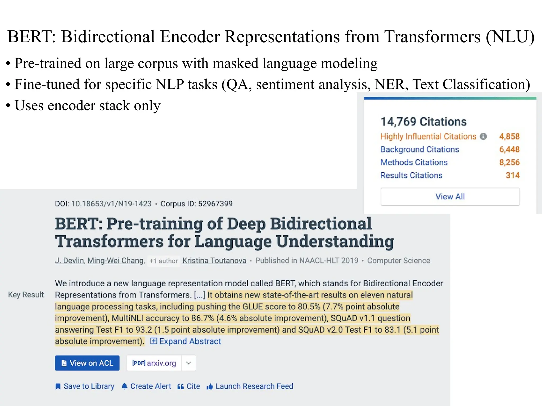
BERT: Bidirectional EncoderRepresentations from Transformers (NLU)
• Pre-trained on large corpus with masked language modeling
• Fine-tuned for specific NLP tasks (QA, sentiment analysis, NER, Text Classification)
• Uses encoder stack only
41.
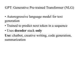
GPT: Generative Pre-trainedTransformer (NLG)
• Autoregressive language model for text
generation
• Trained to predict next token in a sequence
• Uses decoder stack only
Use: chatbot, creative writing, code generation,
summarization
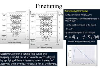
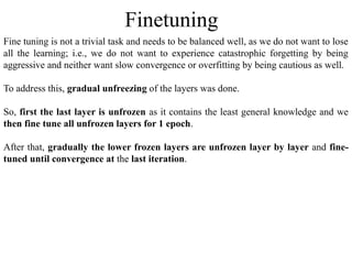
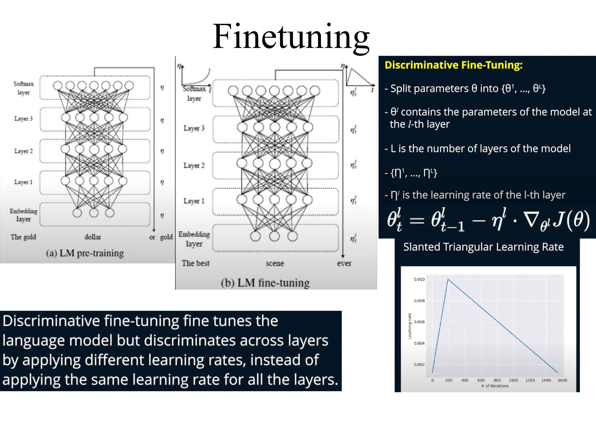
Fine tuning isnot a trivial task and needs to be balanced well, as we do not want to lose
all the learning; i.e., we do not want to experience catastrophic forgetting by being
aggressive and neither want slow convergence or overfitting by being cautious as well.
To address this, gradual unfreezing of the layers was done.
So, first the last layer is unfrozen as it contains the least general knowledge and we
then fine tune all unfrozen layers for 1 epoch.
After that, gradually the lower frozen layers are unfrozen layer by layer and fine-
tuned until convergence at the last iteration.
Finetuning
44.
Fine-tuning Transformer Models
•Use pre-trained models from HuggingFace
Transformers
• Add task-specific output layers
• Train with task-specific data using Transfer
Learning
45.
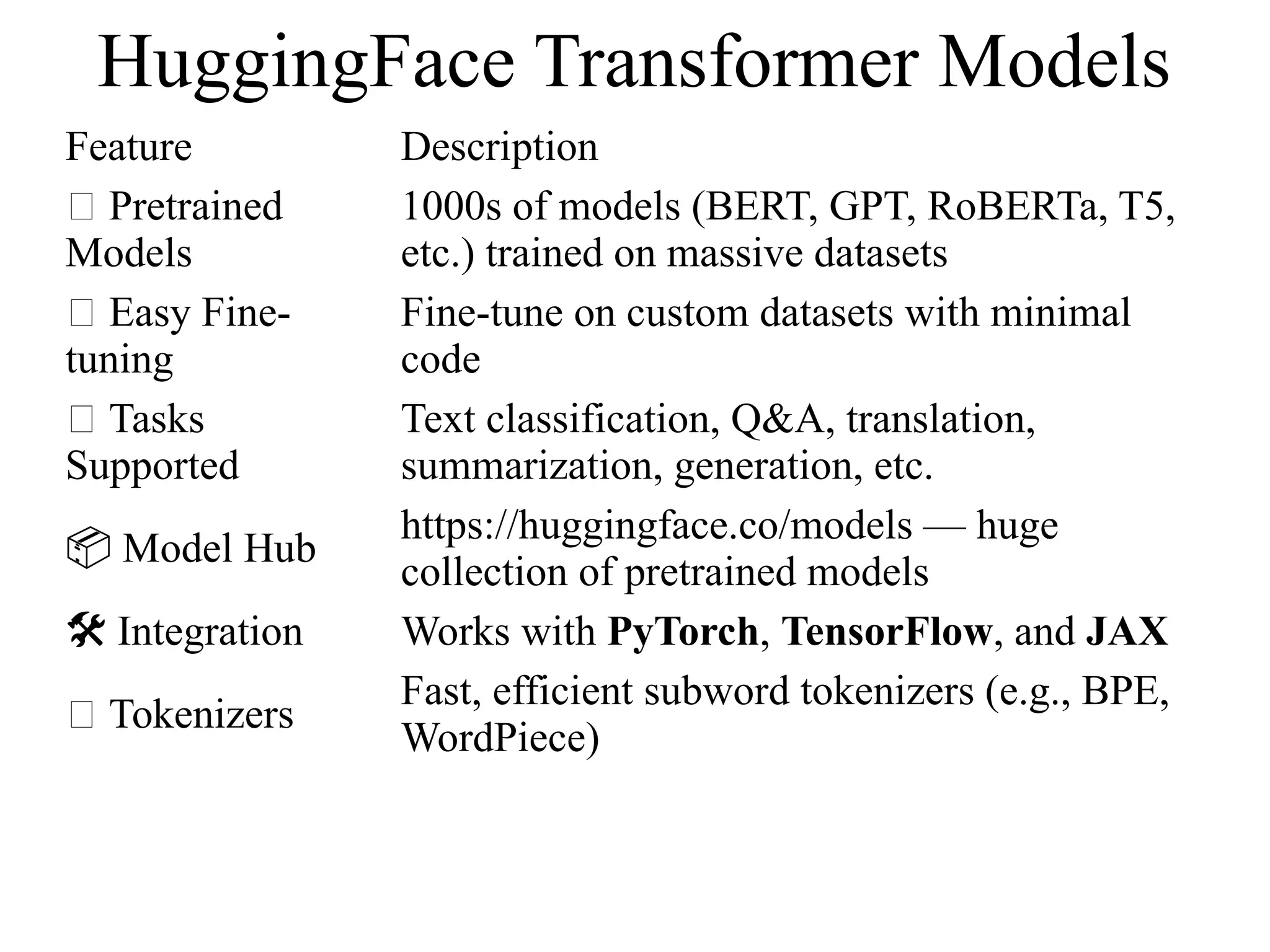
Feature Description
✅ Pretrained
Models
1000sof models (BERT, GPT, RoBERTa, T5,
etc.) trained on massive datasets
🔄 Easy Fine-
tuning
Fine-tune on custom datasets with minimal
code
🧠 Tasks
Supported
Text classification, Q&A, translation,
summarization, generation, etc.
📦 Model Hub
https://huggingface.co/models — huge
collection of pretrained models
️
🛠️Integration Works with PyTorch, TensorFlow, and JAX
🔁 Tokenizers
Fast, efficient subword tokenizers (e.g., BPE,
WordPiece)
HuggingFace Transformer Models
46.
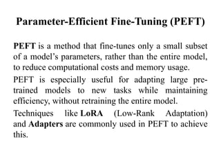
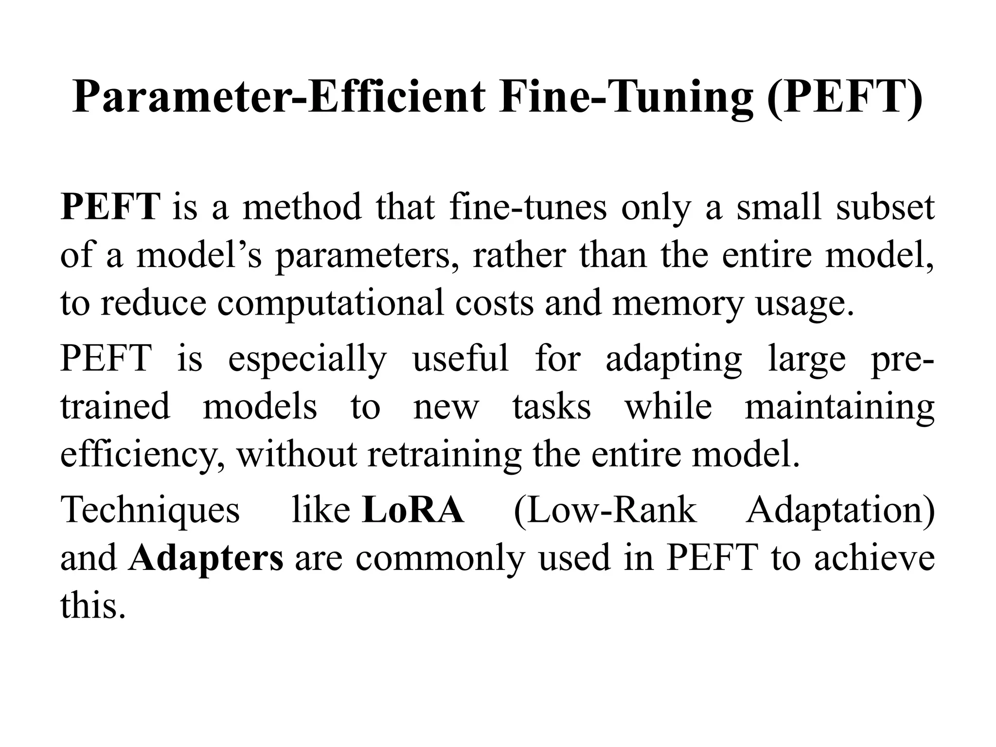
Parameter-Efficient Fine-Tuning (PEFT)
PEFTis a method that fine-tunes only a small subset
of a model’s parameters, rather than the entire model,
to reduce computational costs and memory usage.
PEFT is especially useful for adapting large pre-
trained models to new tasks while maintaining
efficiency, without retraining the entire model.
Techniques like LoRA (Low-Rank Adaptation)
and Adapters are commonly used in PEFT to achieve
this.
47.
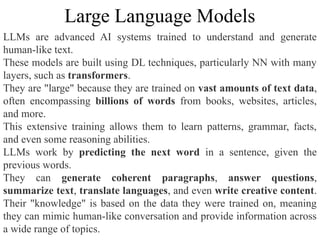
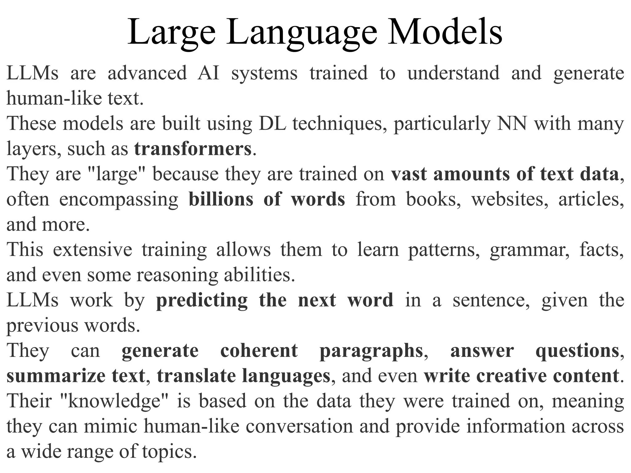
LLMs are advancedAI systems trained to understand and generate
human-like text.
These models are built using DL techniques, particularly NN with many
layers, such as transformers.
They are "large" because they are trained on vast amounts of text data,
often encompassing billions of words from books, websites, articles,
and more.
This extensive training allows them to learn patterns, grammar, facts,
and even some reasoning abilities.
LLMs work by predicting the next word in a sentence, given the
previous words.
They can generate coherent paragraphs, answer questions,
summarize text, translate languages, and even write creative content.
Their "knowledge" is based on the data they were trained on, meaning
they can mimic human-like conversation and provide information across
a wide range of topics.
Large Language Models
48.
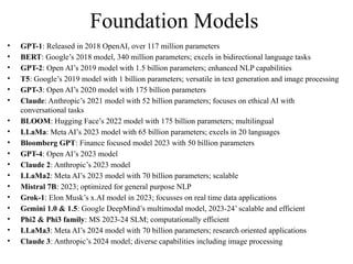
Foundation Models
• GPT-1:Released in 2018 OpenAI, over 117 million parameters
• BERT: Google’s 2018 model, 340 million parameters; excels in bidirectional language tasks
• GPT-2: Open AI’s 2019 model with 1.5 billion parameters; enhanced NLP capabilities
• T5: Google’s 2019 model with 1 billion parameters; versatile in text generation and image processing
• GPT-3: Open AI’s 2020 model with 175 billion parameters
• Claude: Anthropic’s 2021 model with 52 billion parameters; focuses on ethical AI with
conversational tasks
• BLOOM: Hugging Face’s 2022 model with 175 billion parameters; multilingual
• LLaMa: Meta AI’s 2023 model with 65 billion parameters; excels in 20 languages
• Bloomberg GPT: Finance focused model 2023 with 50 billion parameters
• GPT-4: Open AI’s 2023 model
• Claude 2: Anthropic’s 2023 model
• LLaMa2: Meta AI’s 2023 model with 70 billion parameters; scalable
• Mistral 7B: 2023; optimized for general purpose NLP
• Grok-1: Elon Musk’s x.AI model in 2023; focusses on real time data applications
• Gemini 1.0 & 1.5: Google DeepMind’s multimodal model, 2023-24’ scalable and efficient
• Phi2 & Phi3 family: MS 2023-24 SLM; computationally efficient
• LLaMa3: Meta AI’s 2024 model with 70 billion parameters; research oriented applications
• Claude 3: Anthropic’s 2024 model; diverse capabilities including image processing
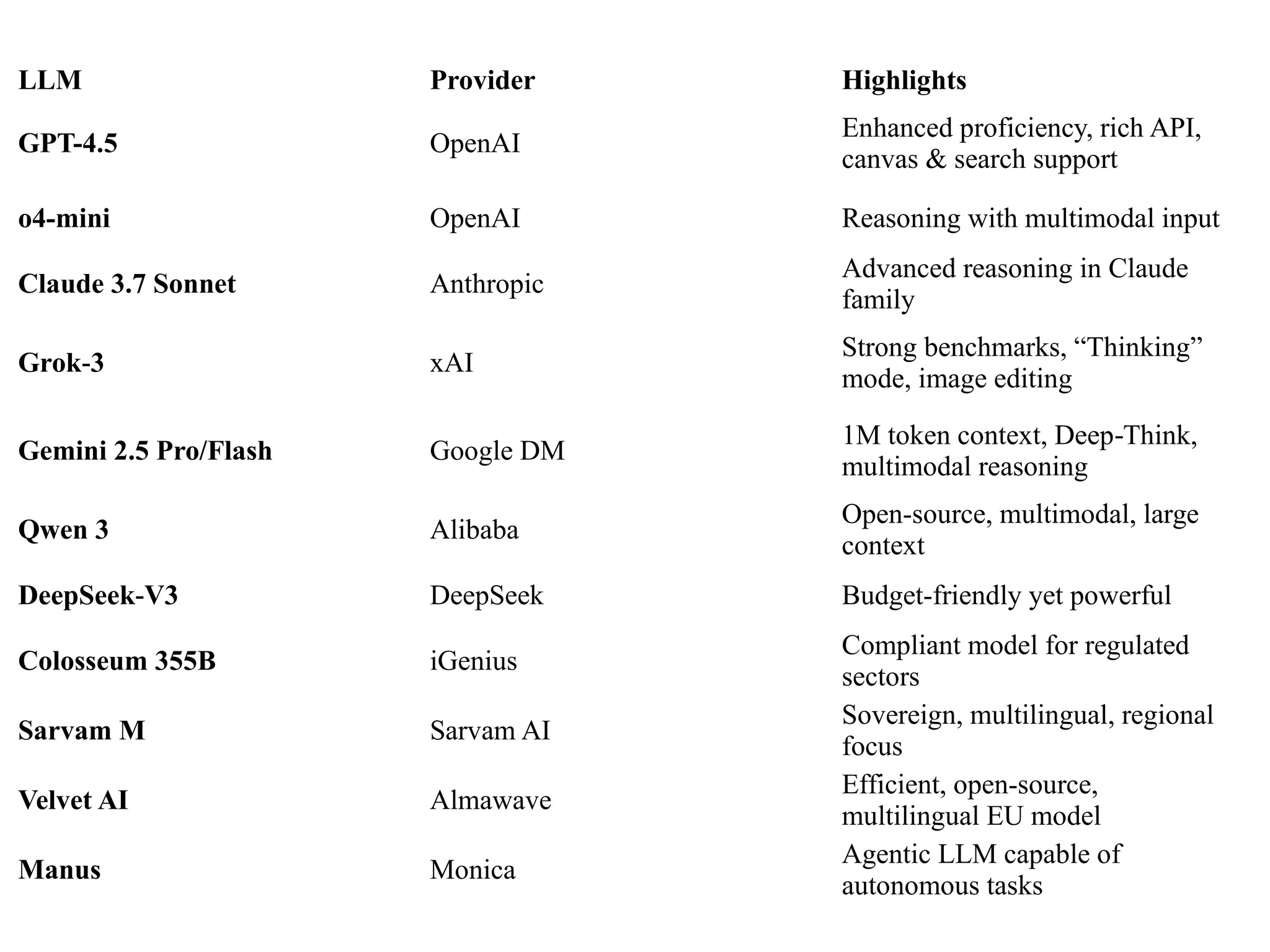
49.
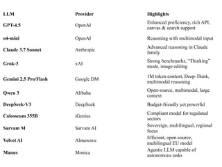
LLM Provider Highlights
GPT-4.5OpenAI
Enhanced proficiency, rich API,
canvas & search support
o4-mini OpenAI Reasoning with multimodal input
Claude 3.7 Sonnet Anthropic
Advanced reasoning in Claude
family
Grok 3
‑ xAI
Strong benchmarks, “Thinking”
mode, image editing
Gemini 2.5 Pro/Flash Google DM
1M token context, Deep Think,
‑
multimodal reasoning
Qwen 3 Alibaba
Open-source, multimodal, large
context
DeepSeek V3
‑ DeepSeek Budget-friendly yet powerful
Colosseum 355B iGenius
Compliant model for regulated
sectors
Sarvam M Sarvam AI
Sovereign, multilingual, regional
focus
Velvet AI Almawave
Efficient, open-source,
multilingual EU model
Manus Monica
Agentic LLM capable of
autonomous tasks
#8 In CBOW architecture the input layer is the context, that is the surrounding words that is both to the left and the right of the target word and is used to predict the target that is the middle word as shown here.
In Skip-Gram Architecture, the input layer is the middle word and is used to predict the context that is the words to the left and the right of the target word as shown here. It is named Skip-Gram because some of the terms or the words are skipped from the context.
#9 sg=1: Use Skip-gram
min_count=1: Include even infrequent words
Learns word vectors where each word predicts its context words.
Each word will output a dense vector (default size = 100 values) learned by the model.
sg=0: Use CBOW — the reverse of skip-gram (context → predict target word)
Each word’s vector typically has 100 dimensions (can be changed via vector_size=100).
#10 This allows you to download and load pre-trained models easily using Gensim’s built-in API
glove-twitter-25 refers to the GloVe embeddings trained on Twitter data with 25 dimensions.
Other versions available include:
'glove-wiki-gigaword-50', 'glove-wiki-gigaword-100', etc.
This returns a model that can be queried like a dictionary to get word vectors.
This retrieves the 25-dimensional vector for the word 'computer'.
[-0.0978 0.1153 -0.1457 ... 0.0562] This vector captures semantic meaning — e.g., "computer" will be close in vector space to "laptop", "technology", or "software".
#16 Lang modeling: next word prediction
Seq to seq task: m/c translation, text summarization, dialogue systems
#18 Benefit Explanation
Stabilizes training Prevents exploding/vanishing gradients
Faster convergence Enables deeper networks to train efficiently
Handles dynamic inputs Unlike batch normalization, it works well with variable sequence lengths
Reduces internal covariate shift Keeps distribution of activations stable as training progresses
#21 concept is very similar to that of the auto encoders which encodes the input information in compressed format and the decoder decodes the same input using the compressed vector representation
#22 Encoder neural network reads and encodes a source sentence into a fixed length vector. A Decoder then outputs a translation from the encoded vector. The whole encoder decoder system which consists of the encoder and the decoder for a language pair is jointly trained to maximize the probability of a correct translation given a source sentence.
Researchers observed encoder-decoder model for neural machine translation performs relatively well on short sentences without unknown words. But its performance degrades rapidly as the length of the sentence and when the number of unknown words increase.
BLEU score increases for short length and as the sentence length increases, the BLEU score decreases
Encoder-Decoder approach compresses all the necessary information of a source length into a fixed length vector
This may make it difficult for the NN to cope with long sentences and this issue is bigger when sentences are longer than sentences in the training corpus.
In the encoder-decoder model without attention mechanism, the encoder was a RNN model which is uni-directional; that is it reads an input sequence x in order starting from the first symbol x1 to the last one xTx.
#33 Data compression technique
Text tokenization algo
Method Used In Characteristics
BPE GPT-2, RoBERTa Merges most frequent pairs
WordPiece BERT Similar to BPE but uses likelihood score
Unigram LM XLNet, T5 Probabilistic model over subwords
SentencePiece T5, ALBERT Language-agnostic, supports BPE & Unigram
#35 1. Token Embedding
What it is: A lookup of the input word/subword (e.g., from Byte Pair Encoding or WordPiece) into a dense vector representation.
Why it’s used: It provides semantic meaning of each token (word/subword).
Example:
Input: "I love NLP"
Tokens: ["I", "love", "N", "##LP"]
Each token maps to a unique vector: E("I"), E("love"), E("N"), E("##LP")
2. Segment Embedding (also called Token Type Embedding)
What it is: A vector that indicates which sentence a token belongs to, typically used in models like BERT for tasks involving sentence pairs (e.g., Question Answering, Next Sentence Prediction).
Why it’s used: Helps the model distinguish between multiple parts of the input (e.g., sentence A vs sentence B).
Example:
Input: [CLS] I love NLP [SEP] Transformers are powerful [SEP]
Segment A (0): [CLS] I love NLP [SEP]
Segment B (1): Transformers are powerful [SEP]
Segment embeddings: All tokens from Sentence A get E_A, tokens from Sentence B get E_B
3. Position Embedding
What it is: A vector that encodes the position of each token in the sequence.
Why it’s used: Transformers have no inherent sense of order, so position embeddings provide information about word order.
Two types:
Learned Position Embedding (used in BERT)
Fixed (Sinusoidal) Position Embedding (used in original Transformer paper)
Example:
Tokens: ["I", "love", "NLP"]
Positions: 0, 1, 2
Position embedding adds unique vector P(0), P(1), P(2)
Final Input Embedding to Transformer
For each token at position i, the final input vector is:
Inputi=TokenEmbeddingi+SegmentEmbeddingi+PositionEmbeddingi
![from gensim.models import Word2Vec
# Sample corpus
corpus = [["I", "love", "this", "movie"],
["This", "movie", "is", "terrible"],
["The", "plot", "is", "confusing"]]
# Skip-gram model
model = Word2Vec(sentences=corpus, min_count=1, sg=1)
# Print word vectors
for word in model.wv.key_to_index:
print(word, model.wv.get_vector(word))
# CBOW model
model = Word2Vec(sentences=corpus, min_count=1, sg=0)
# Print word vectors
for word in model.wv.key_to_index:
print(word, model.wv.get_vector(word))
i [ 0.0156 0.0331 -0.0394 ... 0.0742]
love [-0.0173 0.0469 0.0128 ... 0.0883]
this [ 0.0322 -0.0254 -0.0016 ... 0.0594]
i [-0.0021 0.0511 -0.0423 ... 0.0147]
love [ 0.0144 -0.0389 0.0290 ... 0.0231]
this [-0.0216 0.0374 0.0057 ... -0.0129]](https://image.slidesharecdn.com/advancednlpwithtransformerspptfinal50-250710042642-fa60d14f/85/Advanced_NLP_with_Transformers_PPT_final-50-pptx-9-320.jpg)
![Word Embedding
GloVe – Global Vectors for word representation
The model is trained on multiple data sets including
Wikipedia, Twitter and Common Crawl on billions of
tokens and the embeddings are represented in
different dimension size ranging from 50 to 300.
“glove.6B.zip” file
consider the 50-dimension representation
use the dimension reduction technique like t-SNE
that is, t-Distributed Stochastic Neighbor embedding
to reduce the dimensions to 2 and plot around 500
words on those 2-dimensions
import gensim.downloader as api
glove_model = api.load('glove-twitter-25')
sample_glove_embedding=glove_model['computer'];](https://image.slidesharecdn.com/advancednlpwithtransformerspptfinal50-250710042642-fa60d14f/85/Advanced_NLP_with_Transformers_PPT_final-50-pptx-10-320.jpg)


![import tensorflow as tf
from tensorflow.keras.layers import Layer
class ScaledDotProductAttention(Layer):
def __init__(self):
super(ScaledDotProductAttention, self).__init__()
def call(self, query, key, value, mask=None):
# Step 1: Calculate dot product (QK )
ᵀ
matmul_qk = tf.matmul(query, key, transpose_b=True)
# Step 2: Scale the dot product by sqrt(d_k)
dk = tf.cast(tf.shape(key)[-1], tf.float32) # key dimension
scaled_attention_logits = matmul_qk / tf.math.sqrt(dk)
# Step 3: Apply mask (optional, for padding or future words)
if mask is not None:
scaled_attention_logits += (mask * -1e9) # very negative to nullify softmax
# Step 4: Softmax to get attention weights
attention_weights = tf.nn.softmax(scaled_attention_logits, axis=-1)
# Step 5: Multiply by V (weighted sum of values)
output = tf.matmul(attention_weights, value)
return output, attention_weights
Scaled dot product attention](https://image.slidesharecdn.com/advancednlpwithtransformerspptfinal50-250710042642-fa60d14f/85/Advanced_NLP_with_Transformers_PPT_final-50-pptx-25-320.jpg)
![Initialize Vocabulary
Start with a vocabulary of all characters in the training text.
Tokenize Text as Characters
Example: "low", "lower" → ["l", "o", "w"], ["l", "o", "w", "e", "r"]
Count Pair Frequencies
Count all adjacent pairs of tokens.
Example: ("l", "o"), ("o", "w"), ("w", "e"), etc.
Merge Most Frequent Pair
Merge the pair with the highest frequency into a new symbol.
Example: If ("l", "o") is most frequent → replace it with "lo"
Repeat Steps 3–4
Continue merging the most frequent pairs until you reach a desired vocabulary size.
• Handles Out-of-Vocabulary (OOV) Words: Instead of treating unknown words as <unk>,
BPE breaks them into subword units.
• Reduces Vocabulary Size: Saves memory and speeds up training.
• Captures Morphological Structure: Helps models generalize better across similar words (e.g.,
"play", "playing", "played").
Byte Pair Encoding](https://image.slidesharecdn.com/advancednlpwithtransformerspptfinal50-250710042642-fa60d14f/85/Advanced_NLP_with_Transformers_PPT_final-50-pptx-34-320.jpg)


![from gensim.models import Word2Vec
# Sample corpus
corpus = [["I", "love", "this", "movie"],
["This", "movie", "is", "terrible"],
["The", "plot", "is", "confusing"]]
# Skip-gram model
model = Word2Vec(sentences=corpus, min_count=1, sg=1)
# Print word vectors
for word in model.wv.key_to_index:
print(word, model.wv.get_vector(word))
# CBOW model
model = Word2Vec(sentences=corpus, min_count=1, sg=0)
# Print word vectors
for word in model.wv.key_to_index:
print(word, model.wv.get_vector(word))
i [ 0.0156 0.0331 -0.0394 ... 0.0742]
love [-0.0173 0.0469 0.0128 ... 0.0883]
this [ 0.0322 -0.0254 -0.0016 ... 0.0594]
i [-0.0021 0.0511 -0.0423 ... 0.0147]
love [ 0.0144 -0.0389 0.0290 ... 0.0231]
this [-0.0216 0.0374 0.0057 ... -0.0129]](https://image.slidesharecdn.com/advancednlpwithtransformerspptfinal50-250710042642-fa60d14f/75/Advanced_NLP_with_Transformers_PPT_final-50-pptx-9-2048.jpg)
![Word Embedding
GloVe – Global Vectors for word representation
The model is trained on multiple data sets including
Wikipedia, Twitter and Common Crawl on billions of
tokens and the embeddings are represented in
different dimension size ranging from 50 to 300.
“glove.6B.zip” file
consider the 50-dimension representation
use the dimension reduction technique like t-SNE
that is, t-Distributed Stochastic Neighbor embedding
to reduce the dimensions to 2 and plot around 500
words on those 2-dimensions
import gensim.downloader as api
glove_model = api.load('glove-twitter-25')
sample_glove_embedding=glove_model['computer'];](https://image.slidesharecdn.com/advancednlpwithtransformerspptfinal50-250710042642-fa60d14f/75/Advanced_NLP_with_Transformers_PPT_final-50-pptx-10-2048.jpg)


![import tensorflow as tf
from tensorflow.keras.layers import Layer
class ScaledDotProductAttention(Layer):
def __init__(self):
super(ScaledDotProductAttention, self).__init__()
def call(self, query, key, value, mask=None):
# Step 1: Calculate dot product (QK )
ᵀ
matmul_qk = tf.matmul(query, key, transpose_b=True)
# Step 2: Scale the dot product by sqrt(d_k)
dk = tf.cast(tf.shape(key)[-1], tf.float32) # key dimension
scaled_attention_logits = matmul_qk / tf.math.sqrt(dk)
# Step 3: Apply mask (optional, for padding or future words)
if mask is not None:
scaled_attention_logits += (mask * -1e9) # very negative to nullify softmax
# Step 4: Softmax to get attention weights
attention_weights = tf.nn.softmax(scaled_attention_logits, axis=-1)
# Step 5: Multiply by V (weighted sum of values)
output = tf.matmul(attention_weights, value)
return output, attention_weights
Scaled dot product attention](https://image.slidesharecdn.com/advancednlpwithtransformerspptfinal50-250710042642-fa60d14f/75/Advanced_NLP_with_Transformers_PPT_final-50-pptx-25-2048.jpg)

![Initialize Vocabulary
Start with a vocabulary of all characters in the training text.
Tokenize Text as Characters
Example: "low", "lower" → ["l", "o", "w"], ["l", "o", "w", "e", "r"]
Count Pair Frequencies
Count all adjacent pairs of tokens.
Example: ("l", "o"), ("o", "w"), ("w", "e"), etc.
Merge Most Frequent Pair
Merge the pair with the highest frequency into a new symbol.
Example: If ("l", "o") is most frequent → replace it with "lo"
Repeat Steps 3–4
Continue merging the most frequent pairs until you reach a desired vocabulary size.
• Handles Out-of-Vocabulary (OOV) Words: Instead of treating unknown words as <unk>,
BPE breaks them into subword units.
• Reduces Vocabulary Size: Saves memory and speeds up training.
• Captures Morphological Structure: Helps models generalize better across similar words (e.g.,
"play", "playing", "played").
Byte Pair Encoding](https://image.slidesharecdn.com/advancednlpwithtransformerspptfinal50-250710042642-fa60d14f/75/Advanced_NLP_with_Transformers_PPT_final-50-pptx-34-2048.jpg)


![Agentic Systems and Compliance - A brief intro [1.2]](https://cdn.slidesharecdn.com/ss_thumbnails/agenticsystemsandcompliace-1-251018025303-958a42ec-thumbnail.jpg?width=600ounds&width=560&fit=bounds)
![Matrix and determinant URT [Autosaved].pptx](https://cdn.slidesharecdn.com/ss_thumbnails/matrixanddeterminanturtautosaved-251018190340-9e6a6deb-thumbnail.jpg?width=600ounds&width=560&fit=bounds)