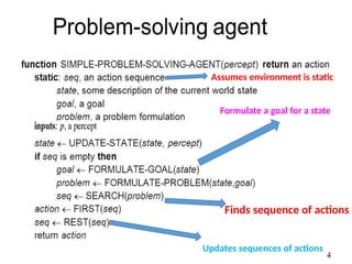
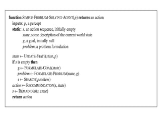
Problem-Solving Agents
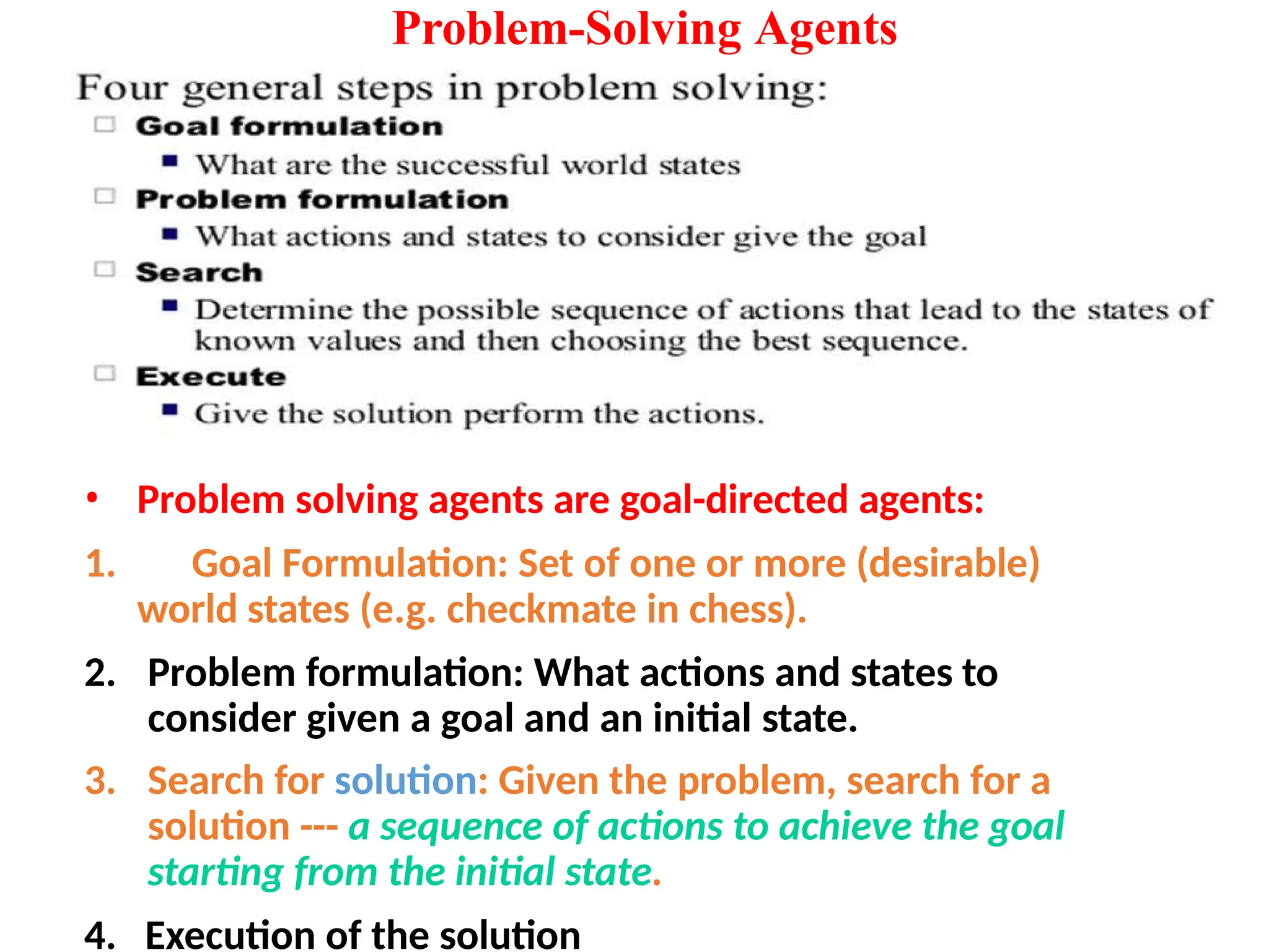
• Problemsolving agents are goal-directed agents:
1. Goal Formulation: Set of one or more (desirable)
world states (e.g. checkmate in chess).
2. Problem formulation: What actions and states to
consider given a goal and an initial state.
3. Search for solution: Given the problem, search for a
solution --- a sequence of actions to achieve the goal
starting from the initial state.
4. Execution of the solution
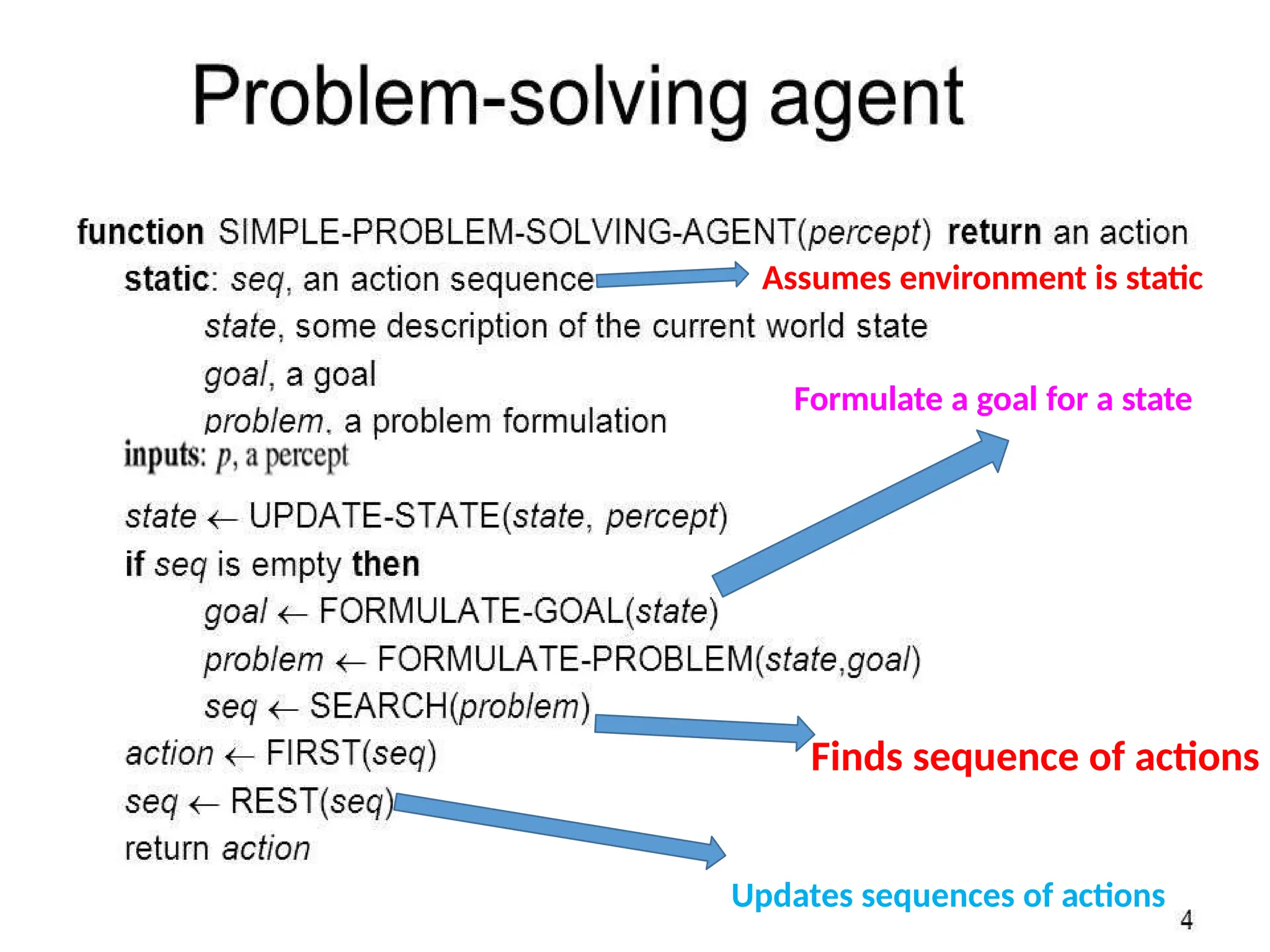
2.
Formulate a goalfor a state
Finds sequence of actions
Updates sequences of actions
Assumes environment is static
4.
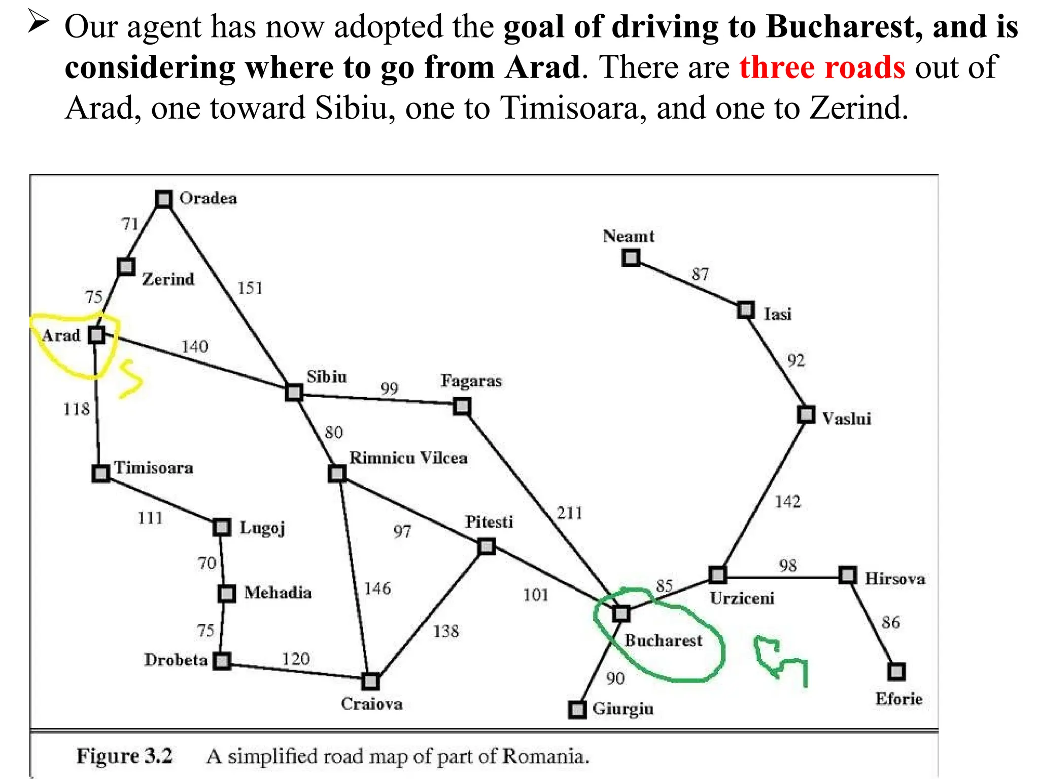
Our agenthas now adopted the goal of driving to Bucharest, and is
considering where to go from Arad. There are three roads out of
Arad, one toward Sibiu, one to Timisoara, and one to Zerind.
5.
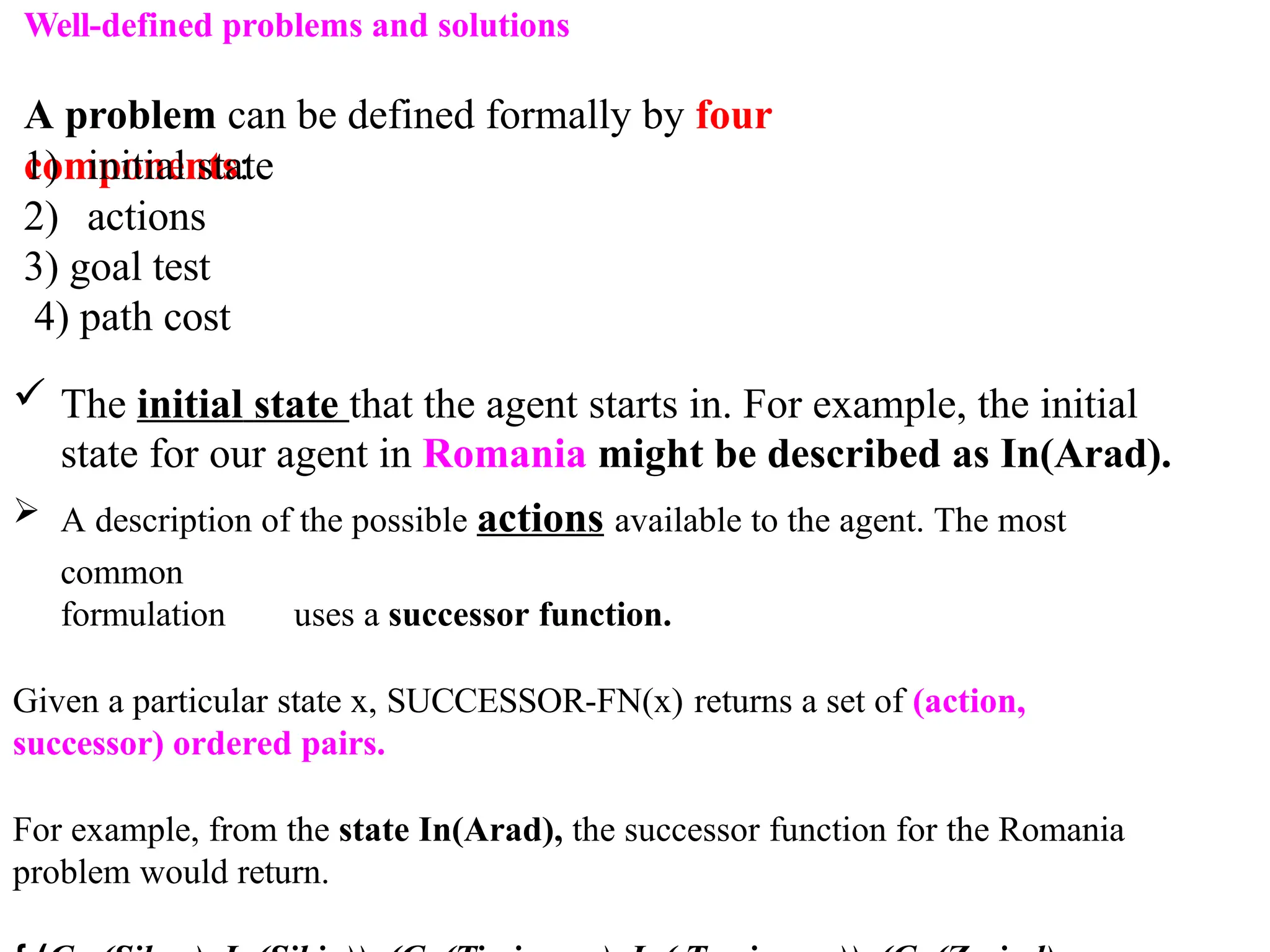
Well-defined problems andsolutions
A problem can be defined formally by four
components:
1) initial state
2) actions
3) goal test
4) path cost
The initial state that the agent starts in. For example, the initial
state for our agent in Romania might be described as In(Arad).
A description of the possible actions available to the agent. The most
common
formulation uses a successor function.
Given a particular state x, SUCCESSOR-FN(x) returns a set of (action,
successor) ordered pairs.
For example, from the state In(Arad), the successor function for the Romania
problem would return.
6.
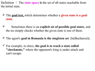
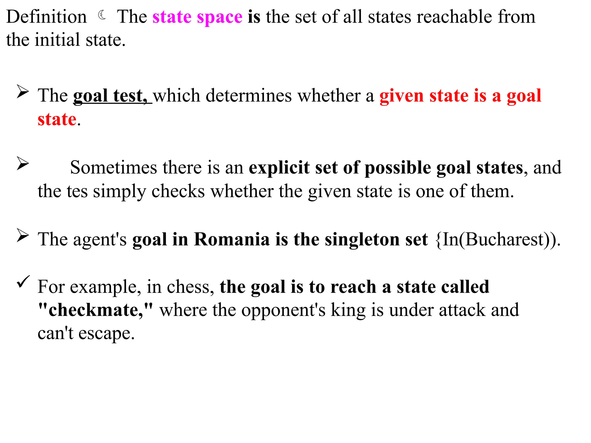
Definition Thestate space is the set of all states reachable from
the initial state.
The goal test, which determines whether a given state is a goal
state.
Sometimes there is an explicit set of possible goal states, and
the tes simply checks whether the given state is one of them.
The agent's goal in Romania is the singleton set {In(Bucharest)).
For example, in chess, the goal is to reach a state called
"checkmate," where the opponent's king is under attack and
can't escape.
7.
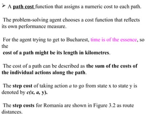
A pathcost function that assigns a numeric cost to each path.
The problem-solving agent chooses a cost function that reflects
its own performance measure.
For the agent trying to get to Bucharest, time is of the essence, so
the
cost of a path might be its length in kilometres.
The cost of a path can be described as the sum of the costs of
the individual actions along the path.
The step cost of taking action a to go from state x to state y is
denoted by c(x, a, y).
The step costs for Romania are shown in Figure 3.2 as route
distances.
8.
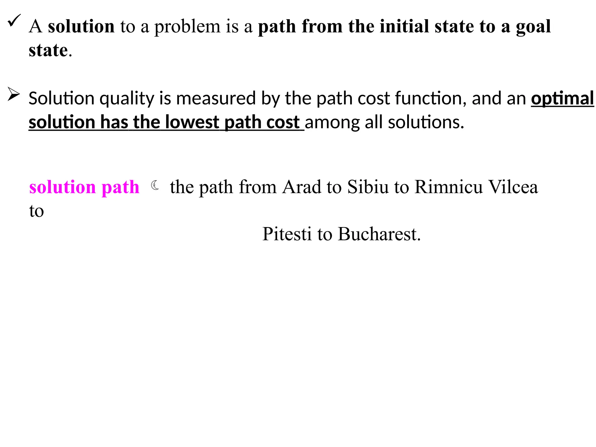
A solutionto a problem is a path from the initial state to a goal
state.
Solution quality is measured by the path cost function, and an optimal
solution has the lowest path cost among all solutions.
solution path the path from Arad to Sibiu to Rimnicu Vilcea
to
Pitesti to Bucharest.
9.
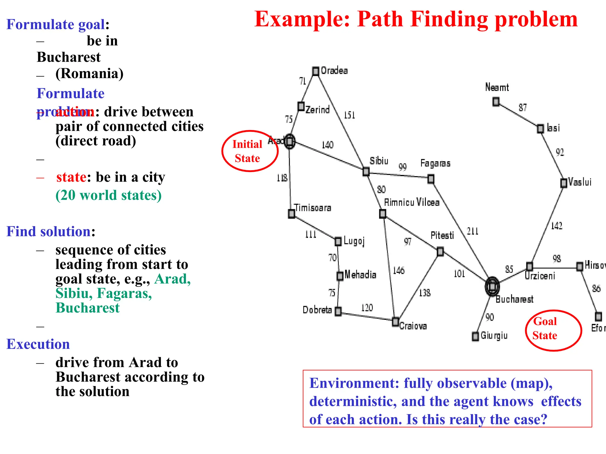
Example: Path Findingproblem
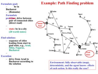
Formulate goal:
– be in
Bucharest
(Romania)
–
Formulate
problem:
– action: drive between
pair of connected cities
(direct road)
–
– state: be in a city
(20 world states)
Find solution:
– sequence of cities
leading from start to
goal state, e.g., Arad,
Sibiu, Fagaras,
Bucharest
–
Execution
– drive from Arad to
Bucharest according to
the solution
Initial
State
Goal
State
Environment: fully observable (map),
deterministic, and the agent knows effects
of each action. Is this really the case?
10.
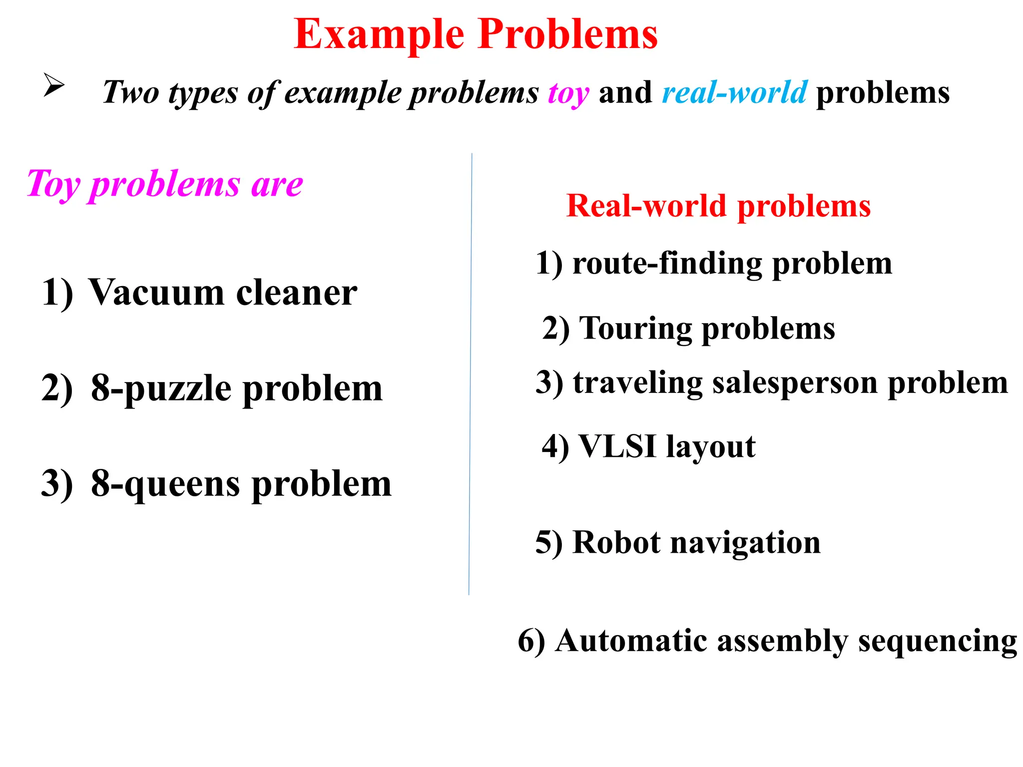
Example Problems
Twotypes of example problems toy and real-world problems
Toy problems are
1) Vacuum cleaner
2) 8-puzzle problem
3) 8-queens problem
5) Robot navigation
6) Automatic assembly sequencing
Real-world problems
1) route-finding problem
2) Touring problems
3) traveling salesperson problem
4) VLSI layout
11.
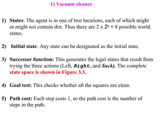
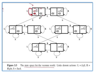
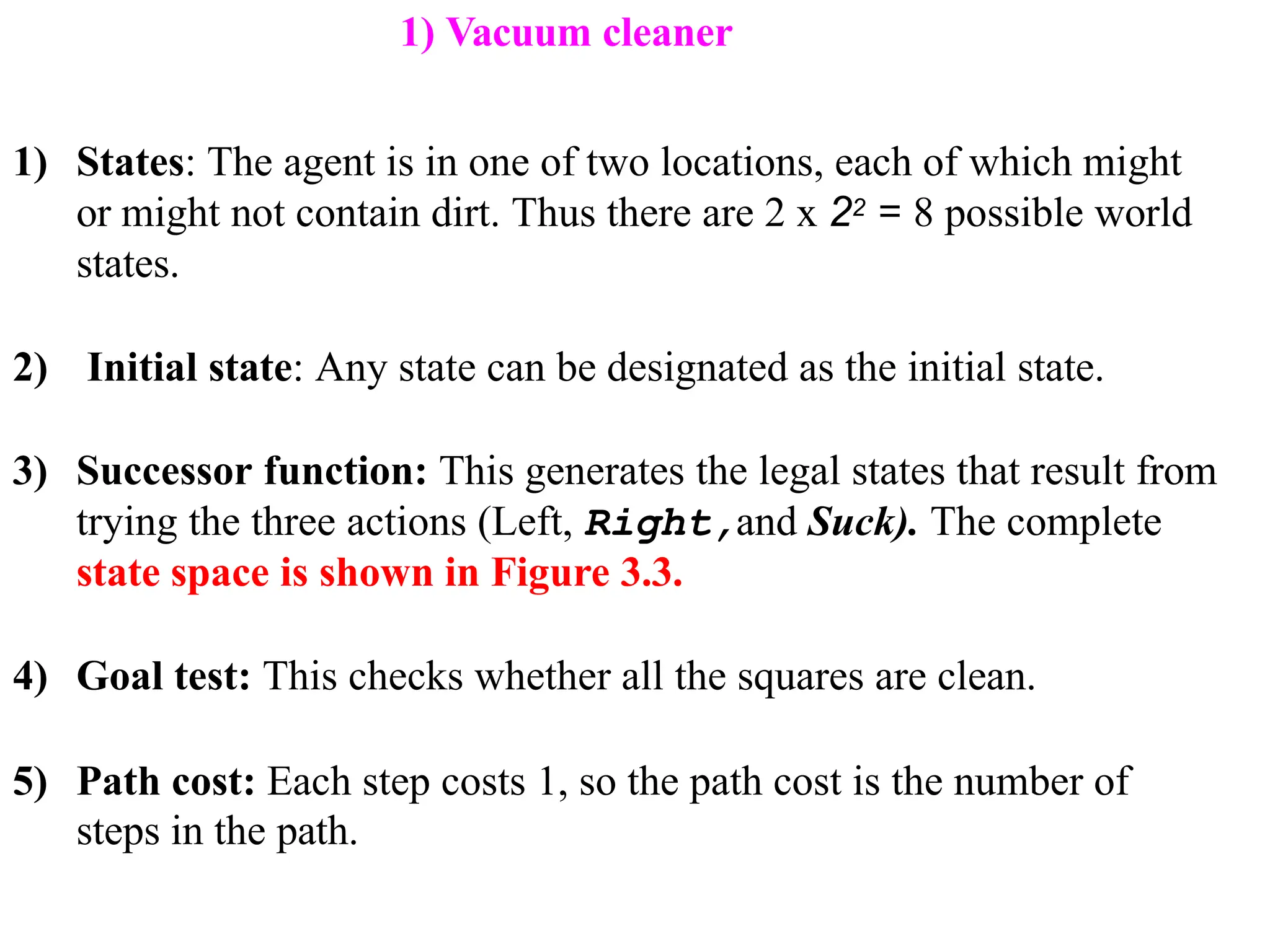
1) States: Theagent is in one of two locations, each of which might
or might not contain dirt. Thus there are 2 x 22 = 8 possible world
states.
2) Initial state: Any state can be designated as the initial state.
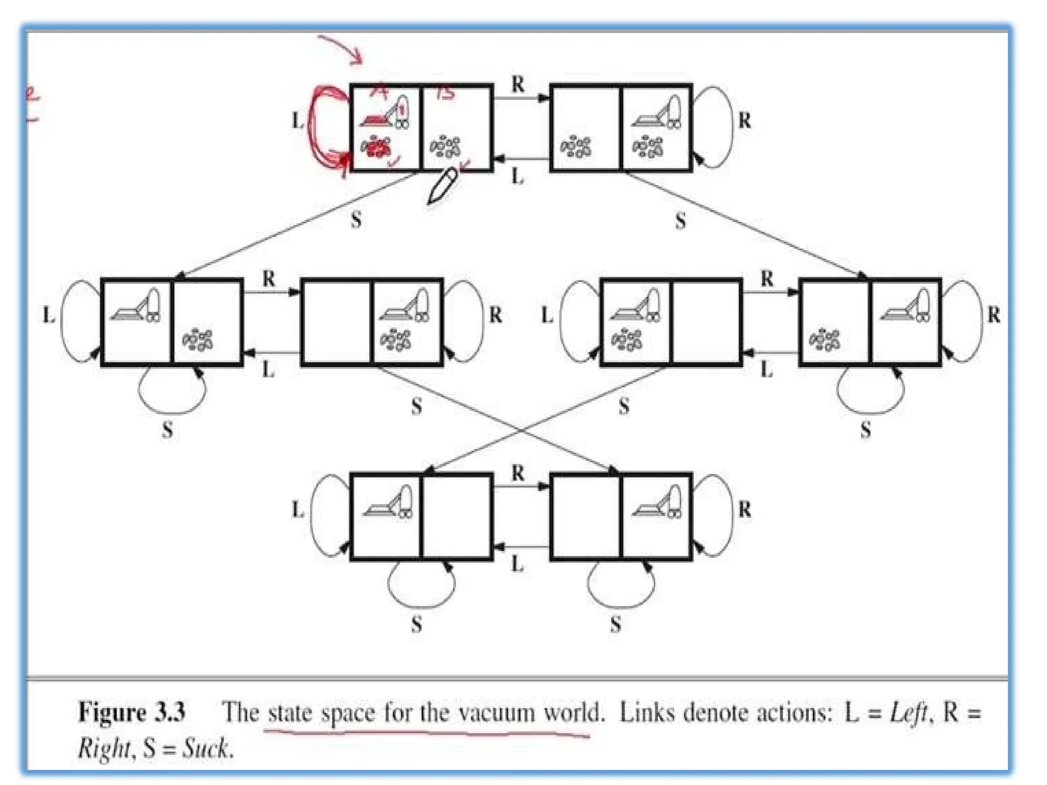
3) Successor function: This generates the legal states that result from
trying the three actions (Left, Right,and Suck). The complete
state space is shown in Figure 3.3.
4) Goal test: This checks whether all the squares are clean.
5) Path cost: Each step costs 1, so the path cost is the number of
steps in the path.
1) Vacuum cleaner
13.
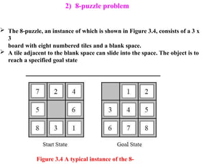
2) 8-puzzle problem
Figure3.4 A typical instance of the 8-
The 8-puzzle, an instance of which is shown in Figure 3.4, consists of a 3 x
3
board with eight numbered tiles and a blank space.
A tile adjacent to the blank space can slide into the space. The object is to
reach a specified goal state
14.
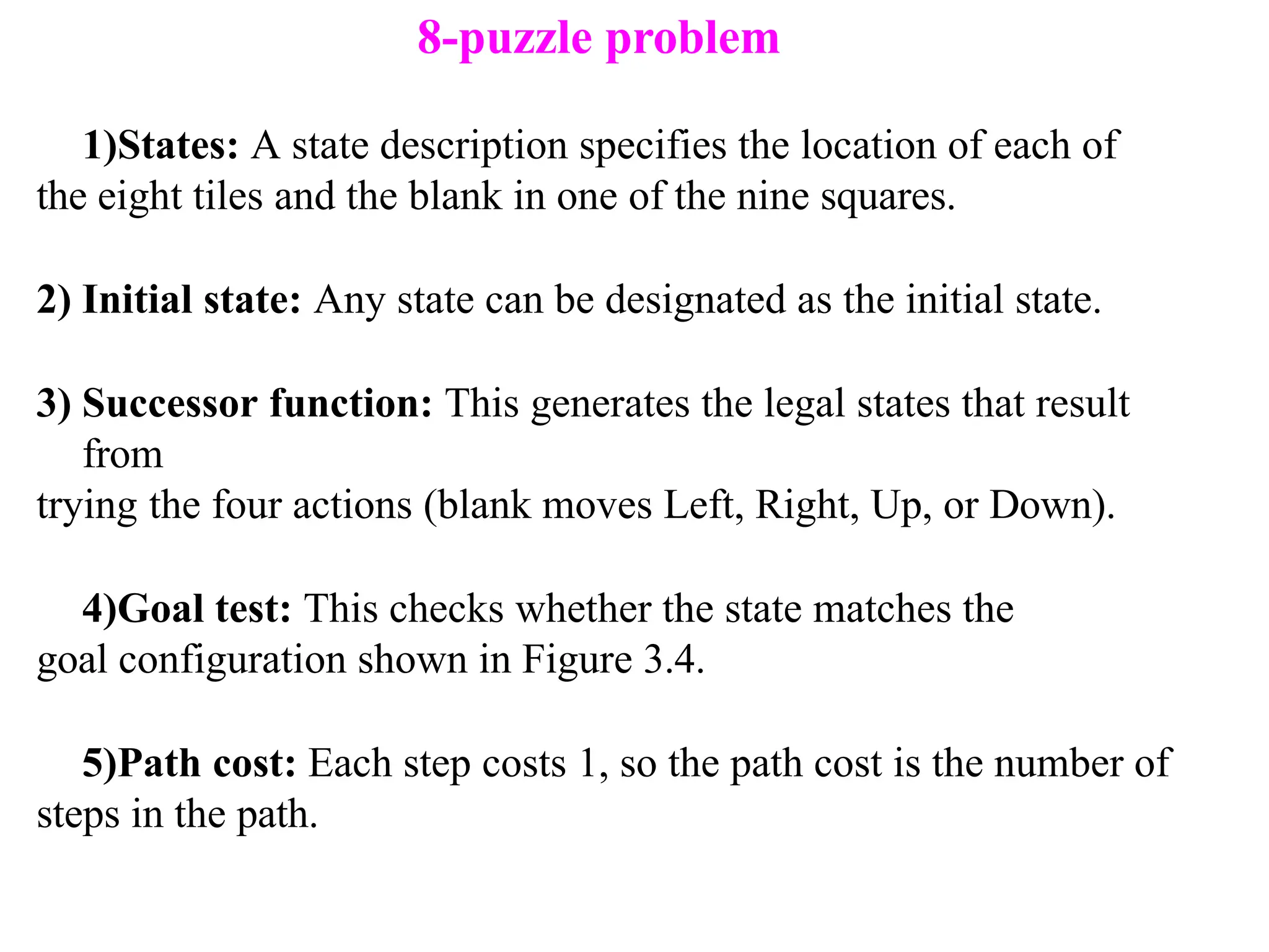
1)States: A statedescription specifies the location of each of
the eight tiles and the blank in one of the nine squares.
2) Initial state: Any state can be designated as the initial state.
3) Successor function: This generates the legal states that result
from
trying the four actions (blank moves Left, Right, Up, or Down).
4)Goal test: This checks whether the state matches the
goal configuration shown in Figure 3.4.
5)Path cost: Each step costs 1, so the path cost is the number of
steps in the path.
8-puzzle problem
15.
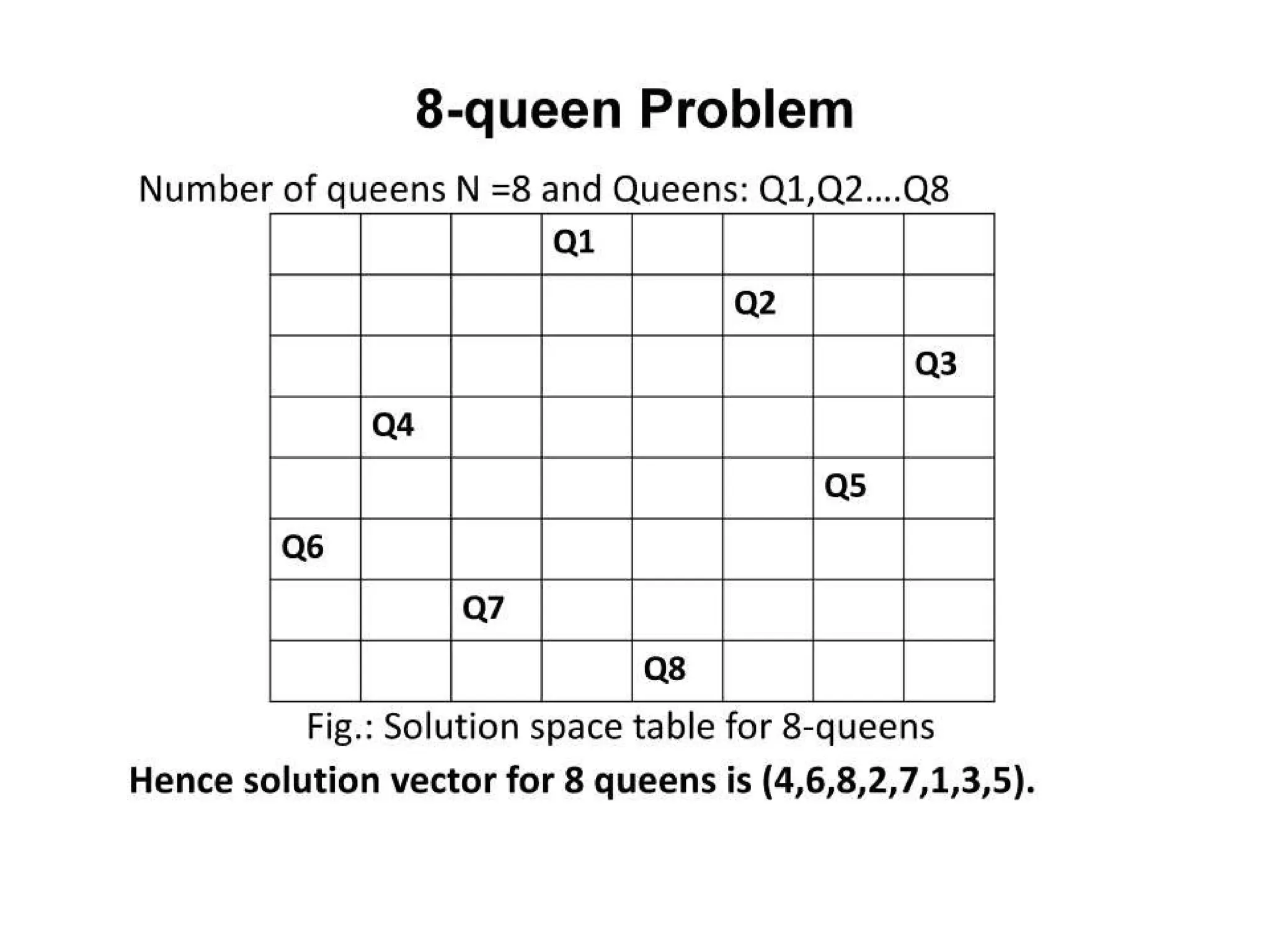
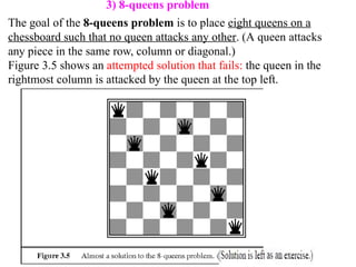
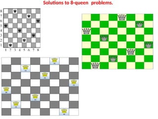
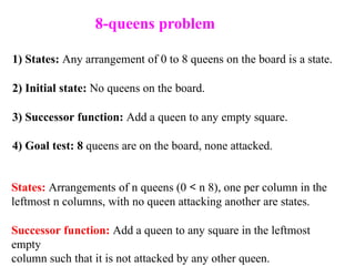
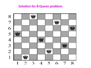
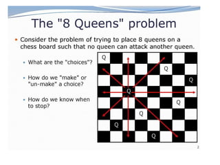
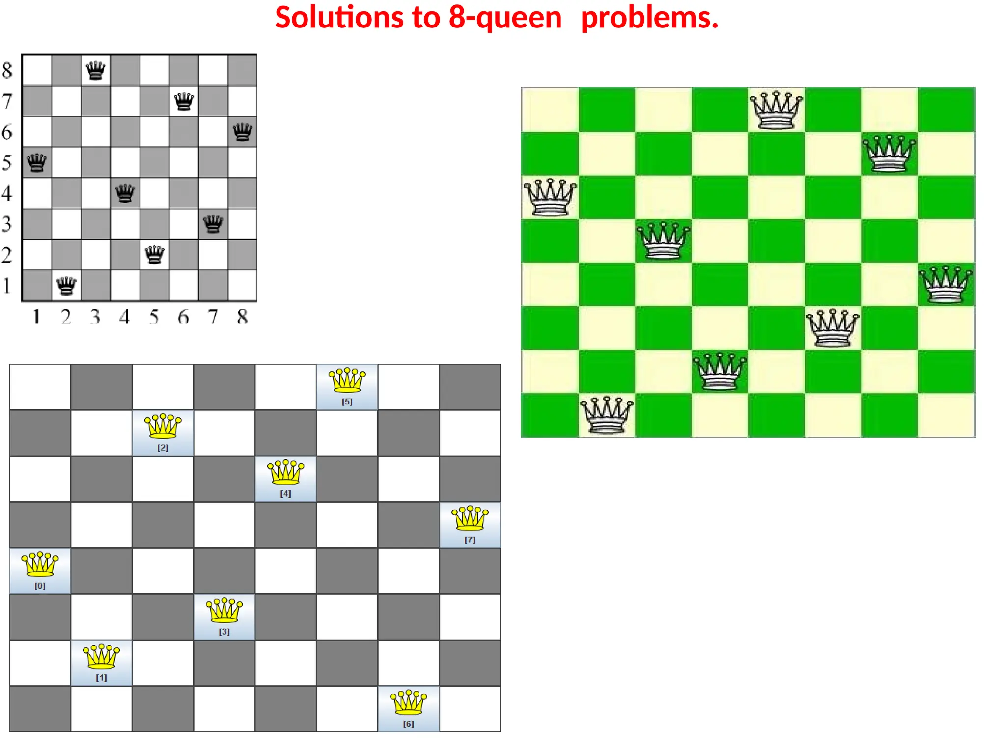
3) 8-queens problem
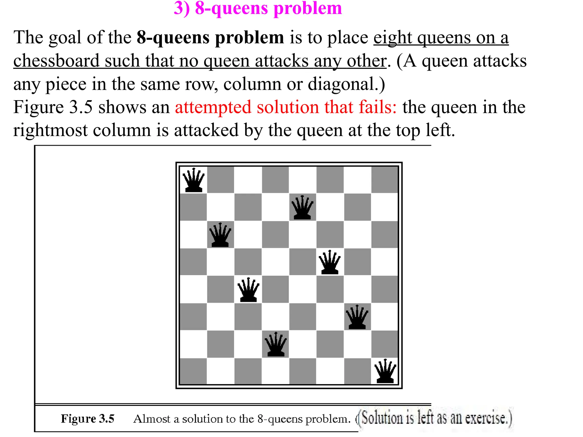
Thegoal of the 8-queens problem is to place eight queens on a
chessboard such that no queen attacks any other. (A queen attacks
any piece in the same row, column or diagonal.)
Figure 3.5 shows an attempted solution that fails: the queen in the
rightmost column is attacked by the queen at the top left.
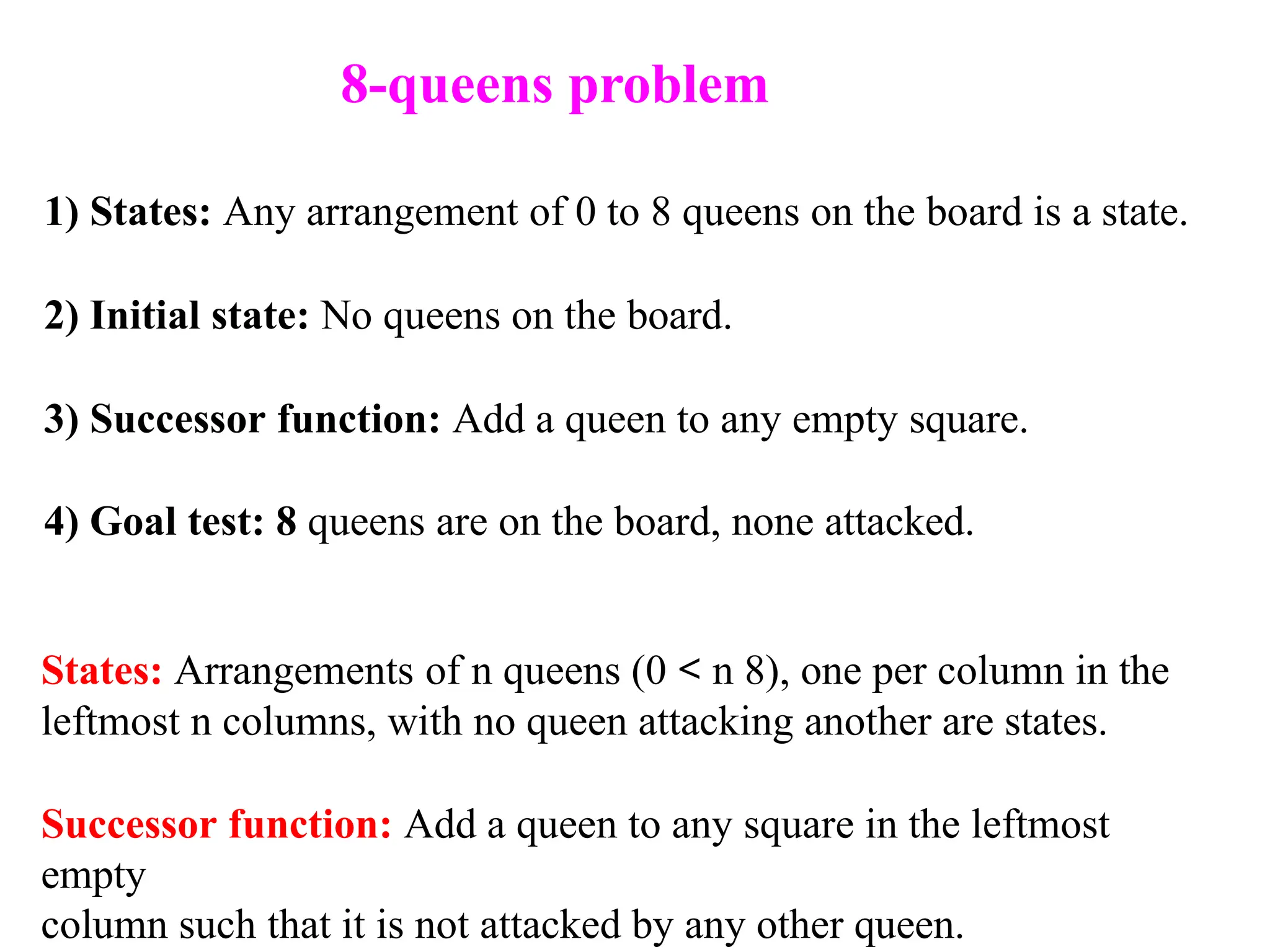
1) States: Anyarrangement of 0 to 8 queens on the board is a state.
2) Initial state: No queens on the board.
3) Successor function: Add a queen to any empty square.
4) Goal test: 8 queens are on the board, none attacked.
States: Arrangements of n queens (0 < n 8), one per column in the
leftmost n columns, with no queen attacking another are states.
Successor function: Add a queen to any square in the leftmost
empty
column such that it is not attacked by any other queen.
8-queens problem
18.
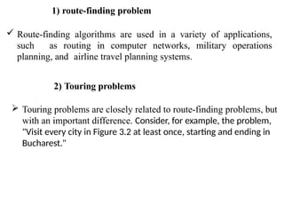
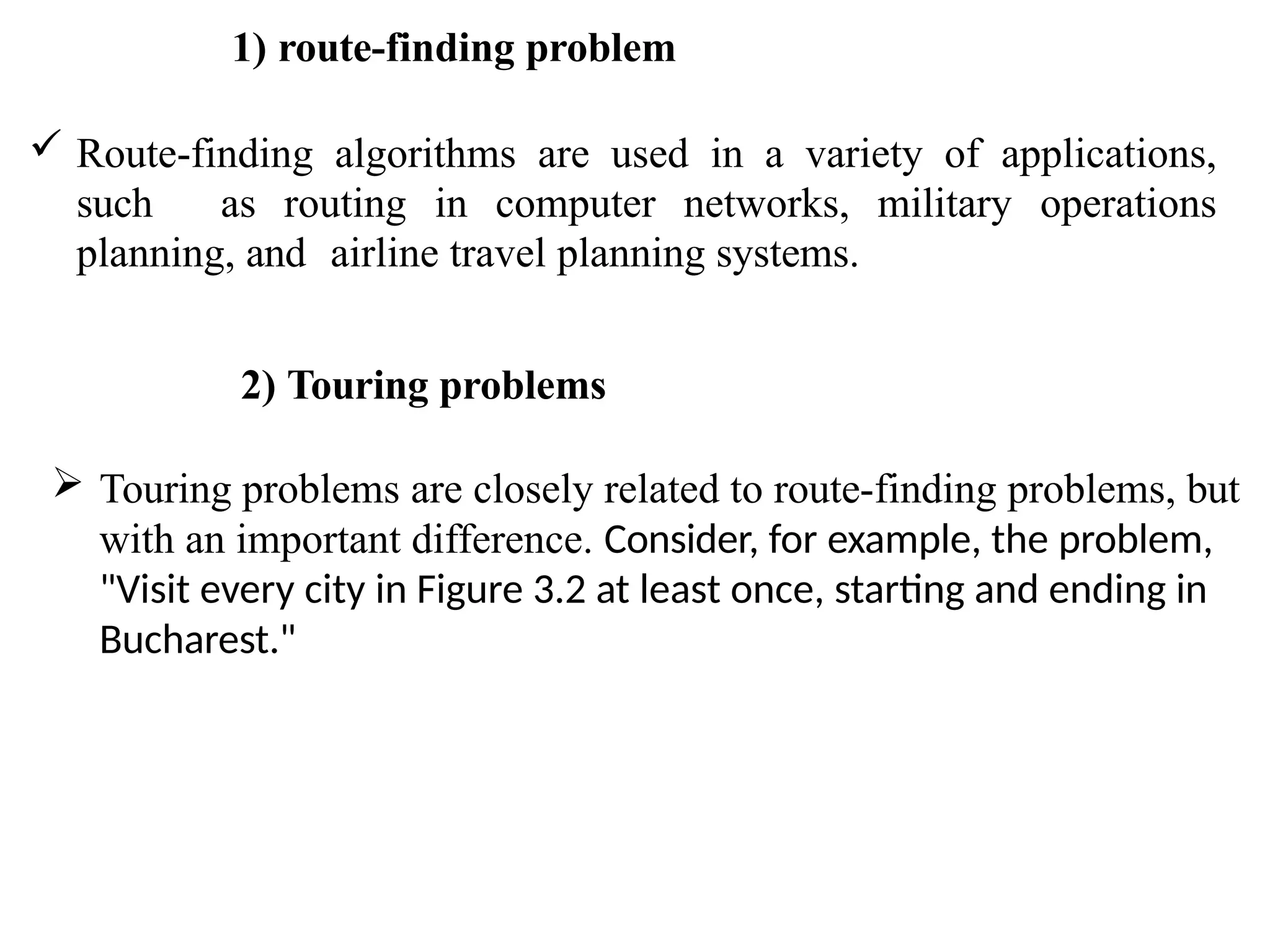
1) route-finding problem
Route-finding algorithms are used in a variety of applications,
such as routing in computer networks, military operations
planning, and airline travel planning systems.
2) Touring problems
Touring problems are closely related to route-finding problems, but
with an important difference. Consider, for example, the problem,
"Visit every city in Figure 3.2 at least once, starting and ending in
Bucharest."
19.
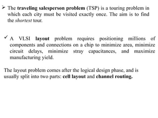
The travelingsalesperson problem (TSP) is a touring problem in
which each city must be visited exactly once. The aim is to find
the shortest tour.
A VLSI layout problem requires positioning millions of
components and connections on a chip to minimize area, minimize
circuit delays, minimize stray capacitances, and maximize
manufacturing yield.
The layout problem comes after the logical design phase, and is
usually split into two parts: cell layout and channel routing.
20.
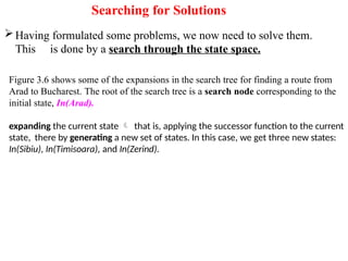
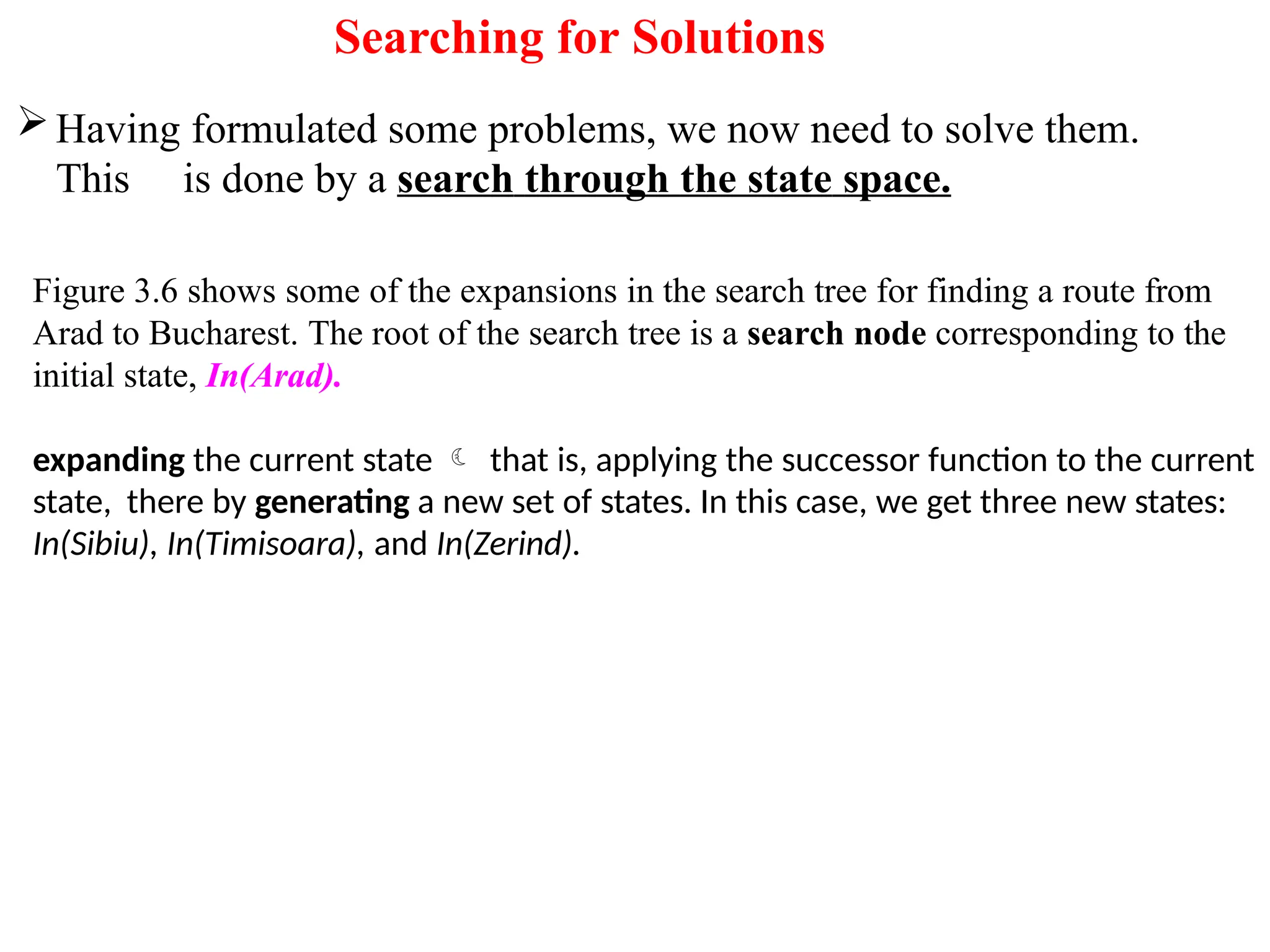
Searching for Solutions
Havingformulated some problems, we now need to solve them.
This is done by a search through the state space.
Figure 3.6 shows some of the expansions in the search tree for finding a route from
Arad to Bucharest. The root of the search tree is a search node corresponding to the
initial state, In(Arad).
expanding the current state that is, applying the successor function to the current
state, there by generating a new set of states. In this case, we get three new states:
In(Sibiu), In(Timisoara), and In(Zerind).
21.
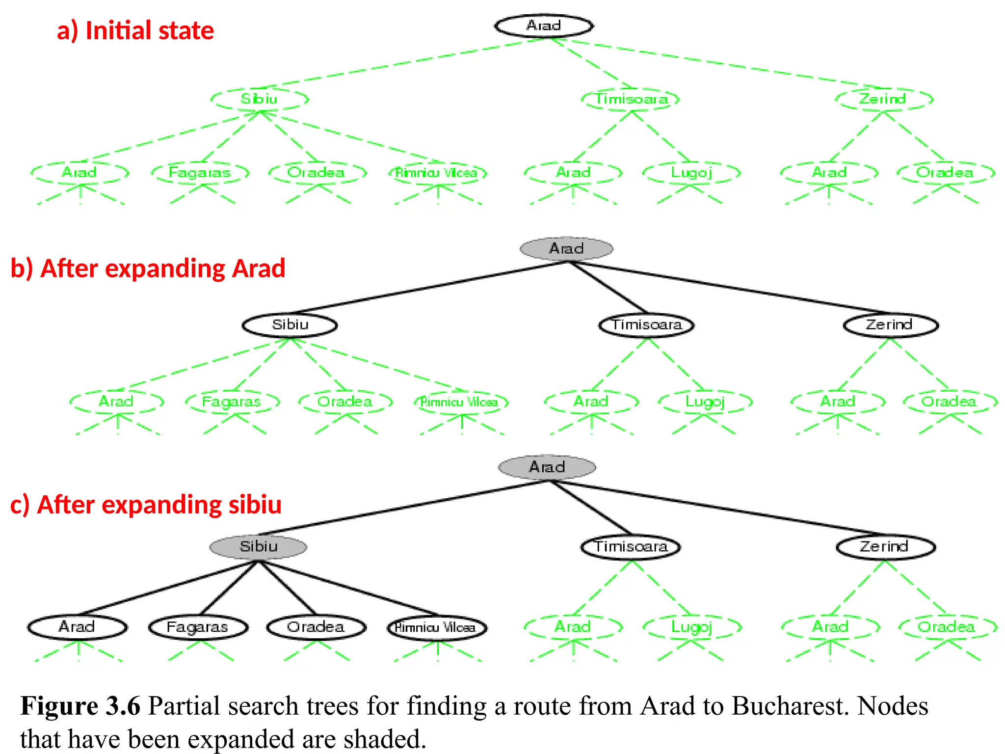
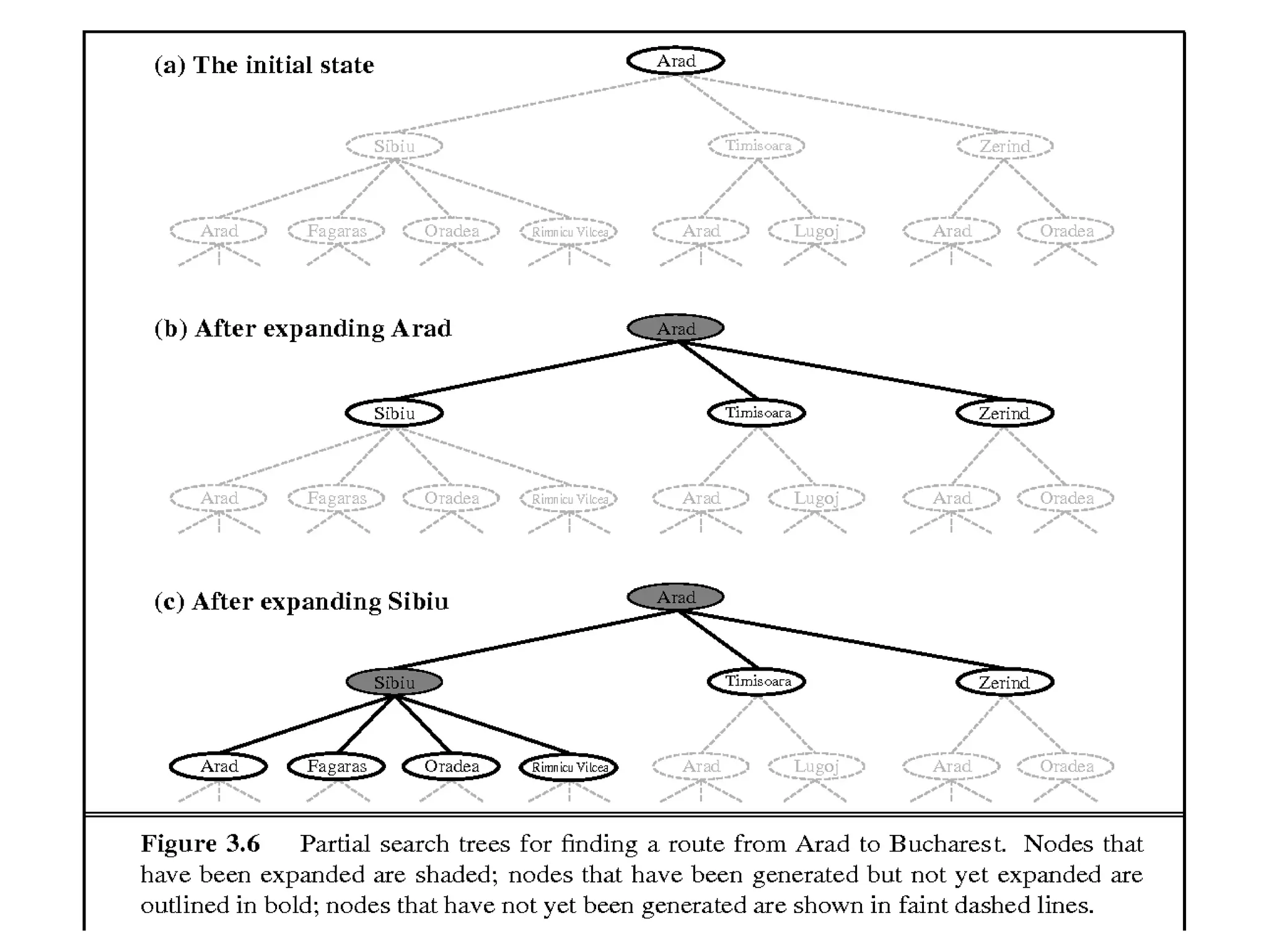
a) Initial state
b)After expanding Arad
c) After expanding sibiu
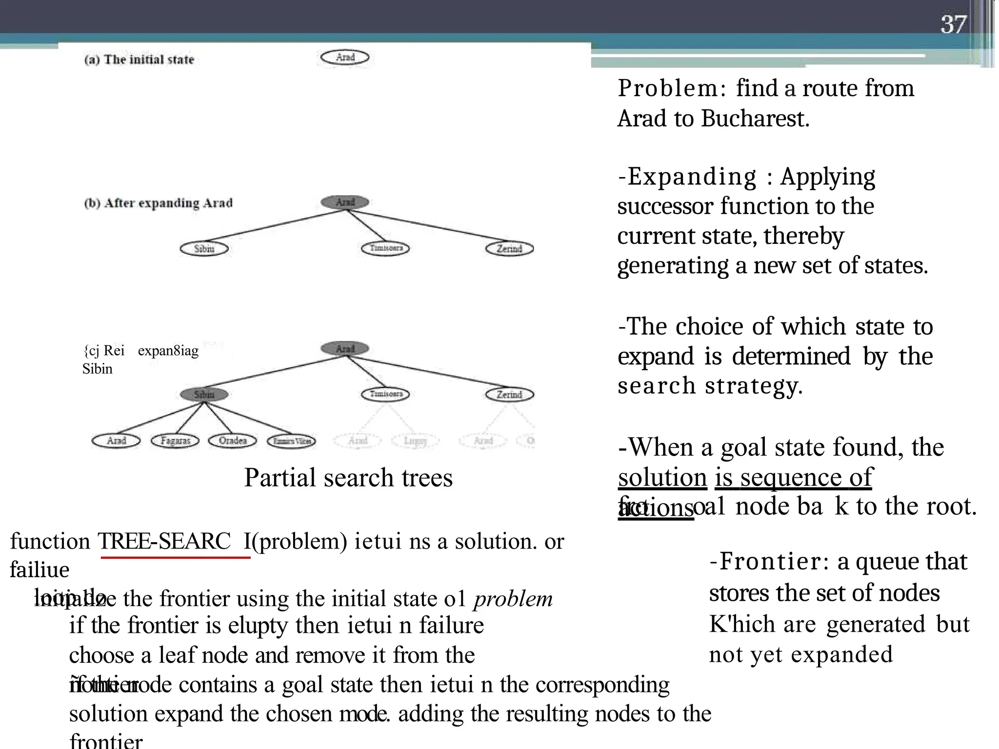
Figure 3.6 Partial search trees for finding a route from Arad to Bucharest. Nodes
that have been expanded are shaded.
23.
{cj Rei expan8iag
Sibin
Partialsearch trees
Problem: find a route from
Arad to Bucharest.
-Expanding : Applying
successor function to the
current state, thereby
generating a new set of states.
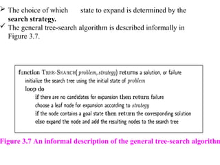
-The choice of which state to
expand is determined by the
search strategy.
-When a goal state found, the
solution is sequence of
actions
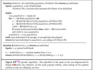
function TREE-SEARC I(problem) ietui ns a solution. or
failiue
initialize the frontier using the initial state o1 problem
loop do
if the frontier is elupty then ietui n failure
choose a leaf node and remove it from the
ñontier
fro oa1 node ba k to the root.
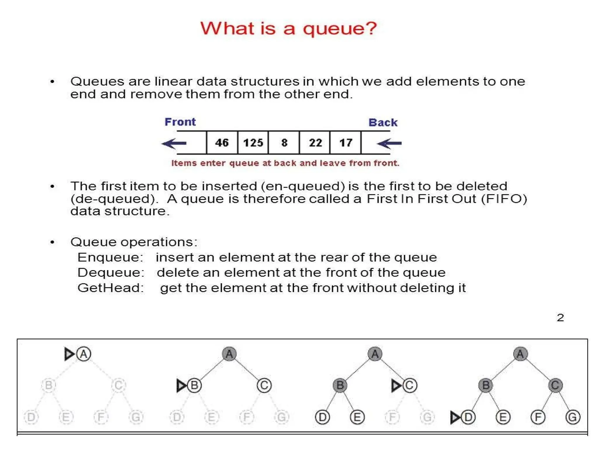
-Frontier: a queue that
stores the set of nodes
K'hich are generated but
not yet expanded
if the node contains a goal state then ietui n the corresponding
solution expand the chosen mode. adding the resulting nodes to the
24.
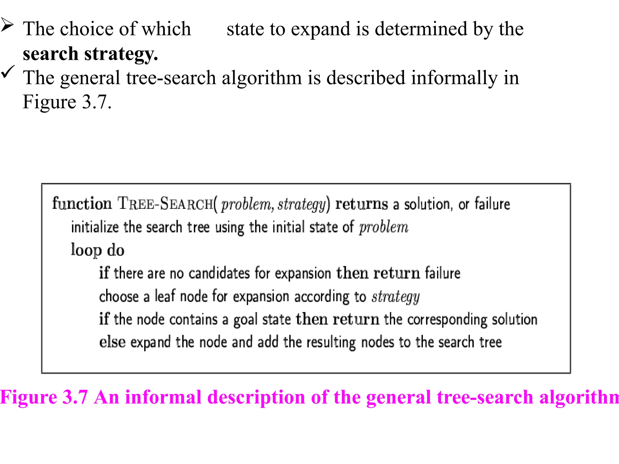
The choiceof which state to expand is determined by the
search strategy.
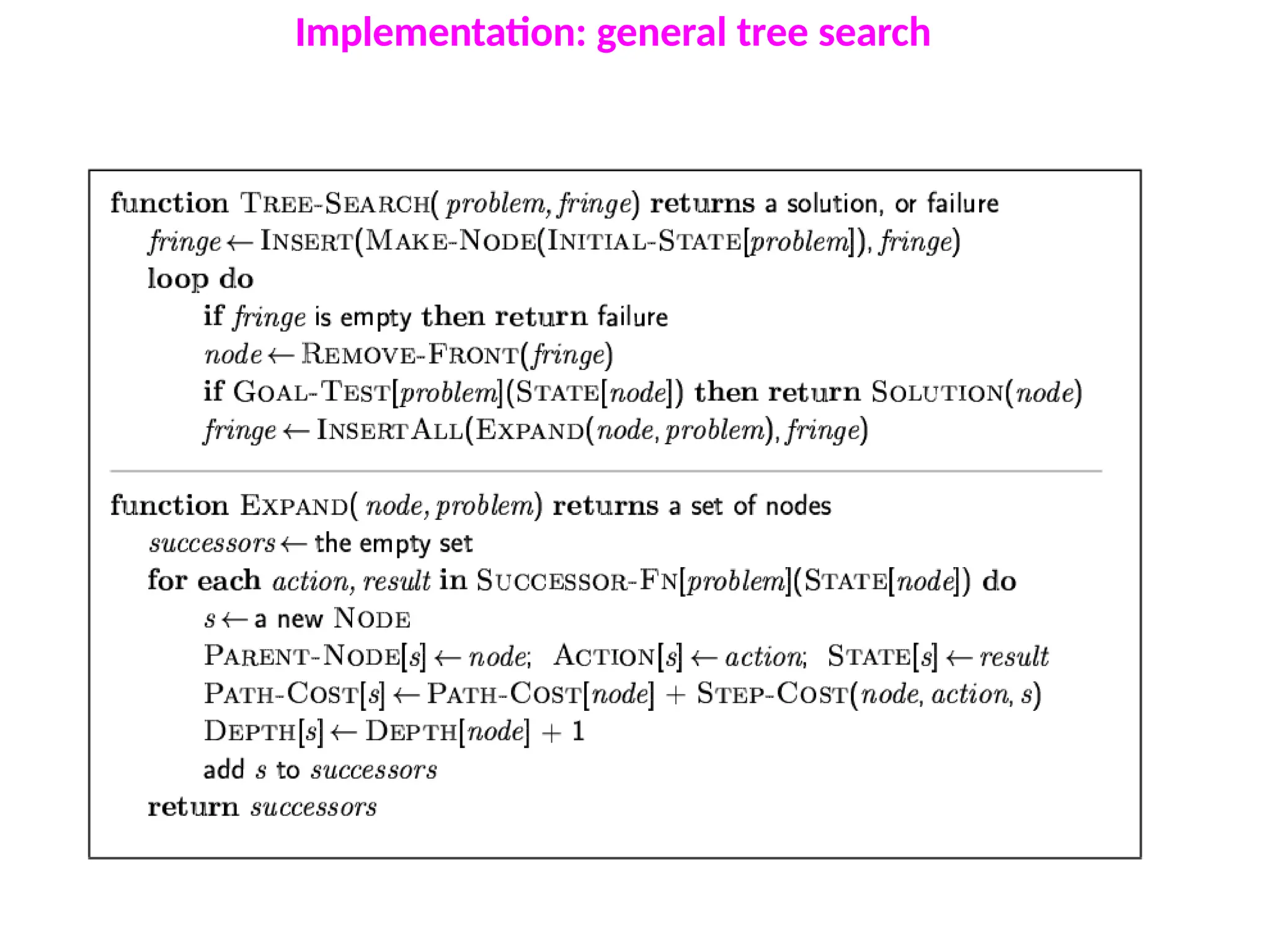
The general tree-search algorithm is described informally in
Figure 3.7.
Figure 3.7 An informal description of the general tree-search algorithm
25.
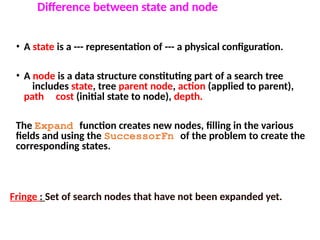
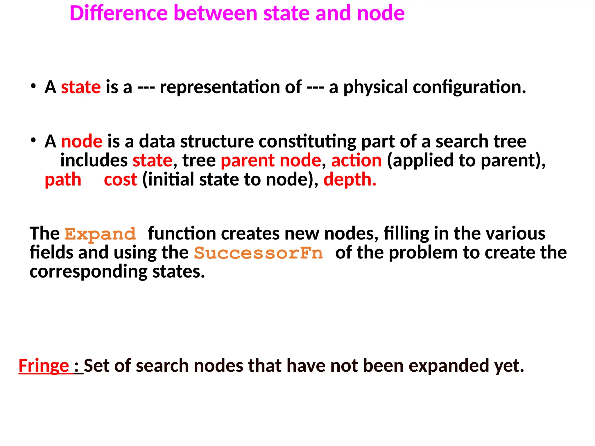
• A stateis a --- representation of --- a physical configuration.
• A node is a data structure constituting part of a search tree
includes state, tree parent node, action (applied to parent),
path cost (initial state to node), depth.
The Expand function creates new nodes, filling in the various
fields and using the SuccessorFn of the problem to create the
corresponding states.
Difference between state and node
Fringe : Set of search nodes that have not been expanded yet.
26.
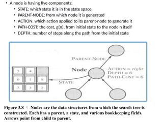
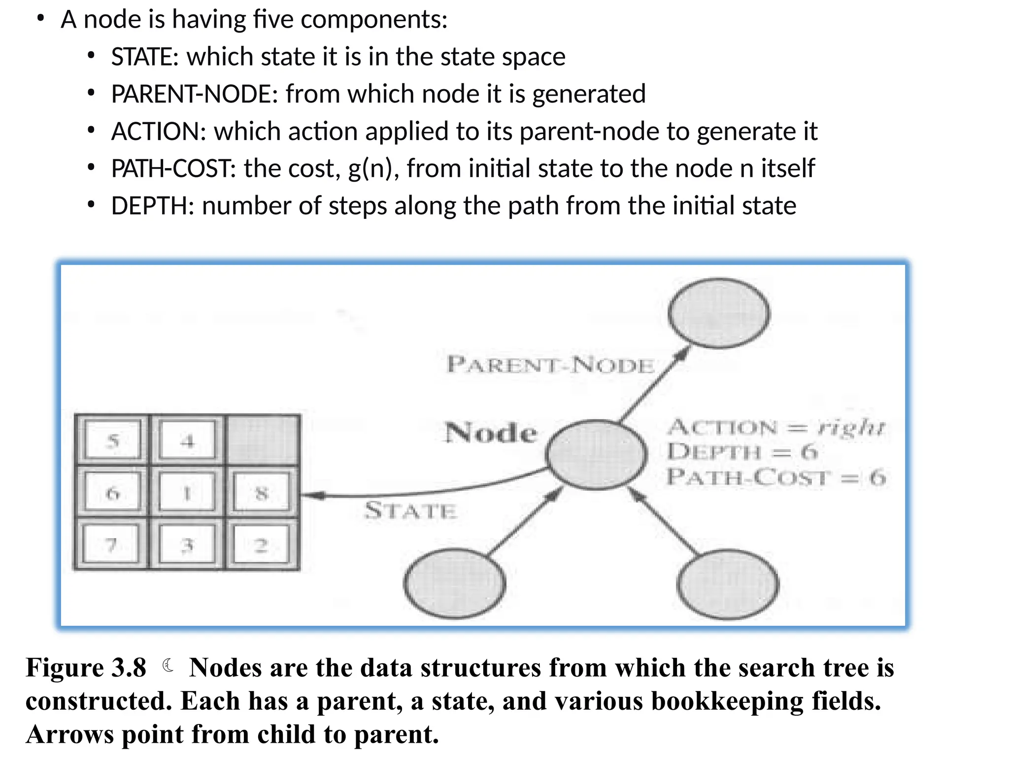
• A nodeis having five components:
• STATE: which state it is in the state space
• PARENT-NODE: from which node it is generated
• ACTION: which action applied to its parent-node to generate it
• PATH-COST: the cost, g(n), from initial state to the node n itself
• DEPTH: number of steps along the path from the initial state
Figure 3.8 Nodes are the data structures from which the search tree is
constructed. Each has a parent, a state, and various bookkeeping fields.
Arrows point from child to parent.
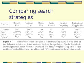
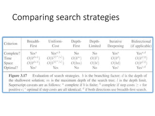
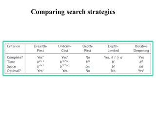
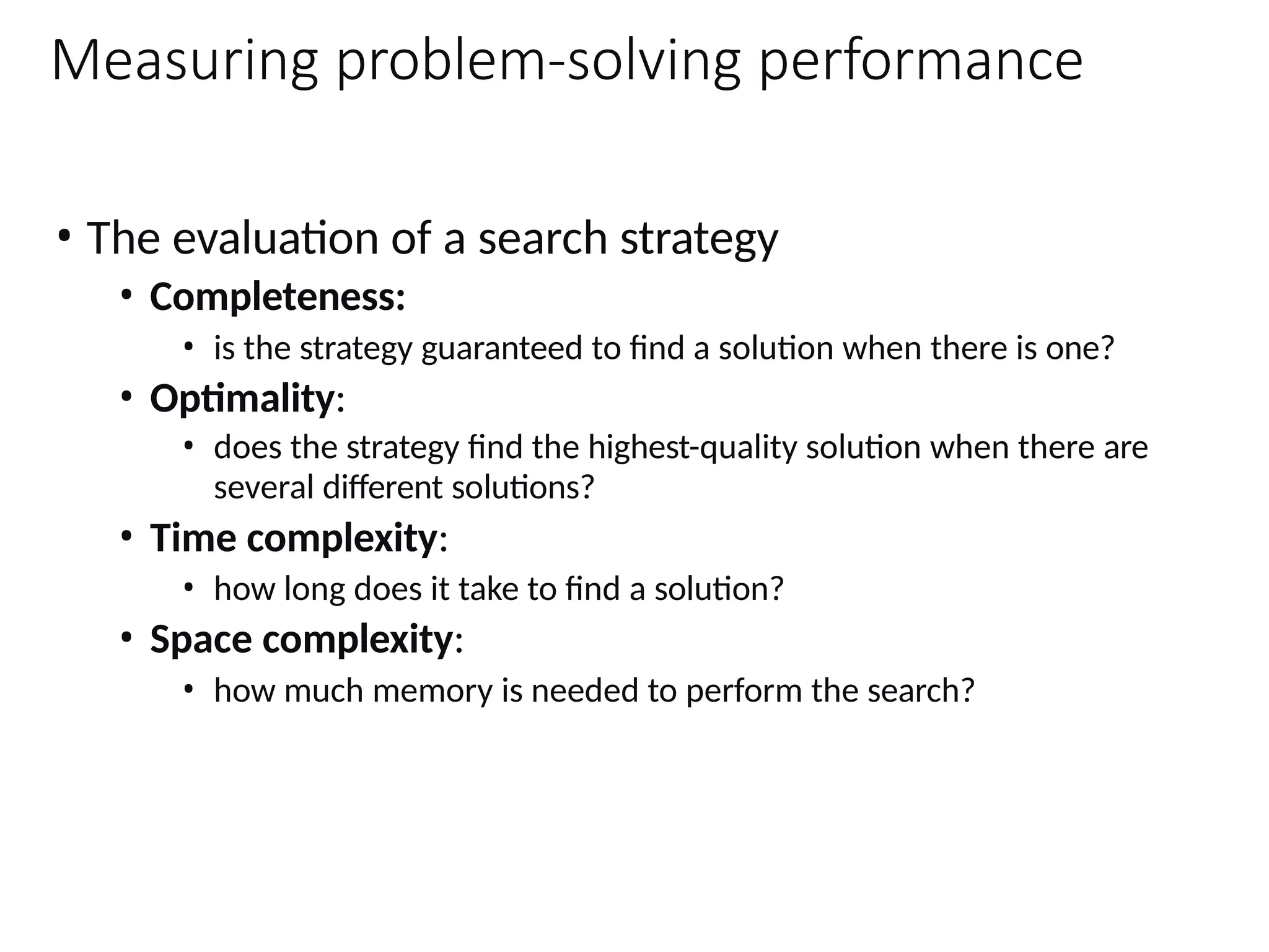
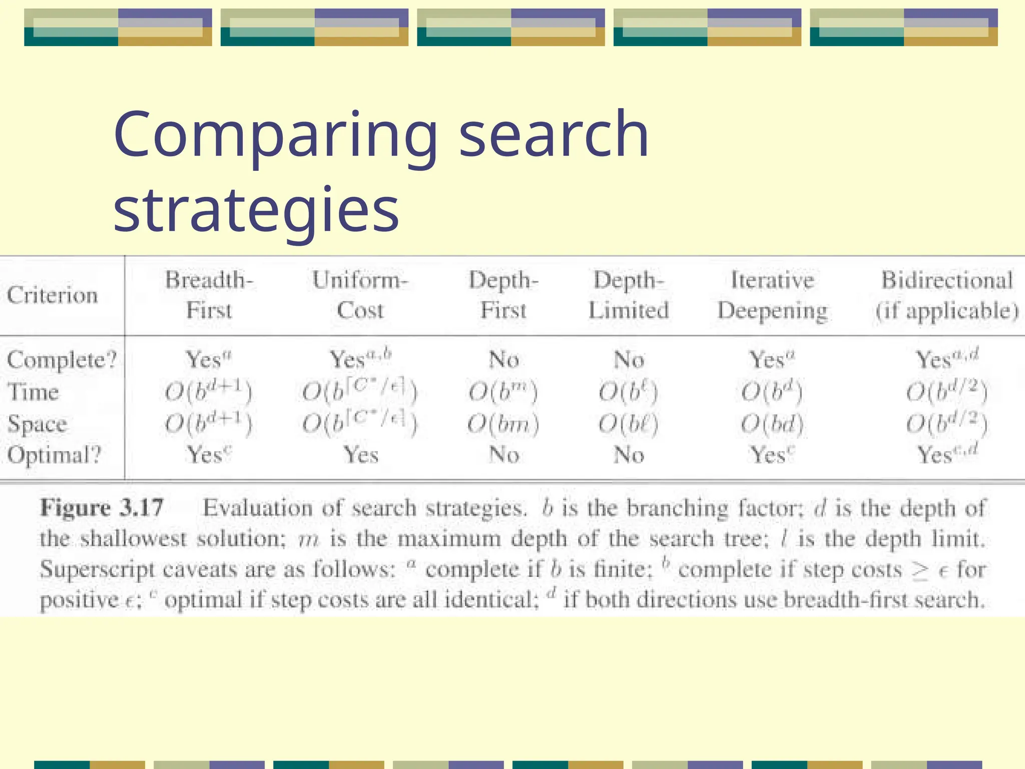
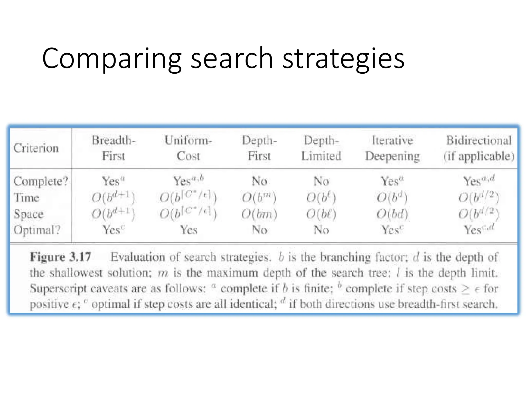
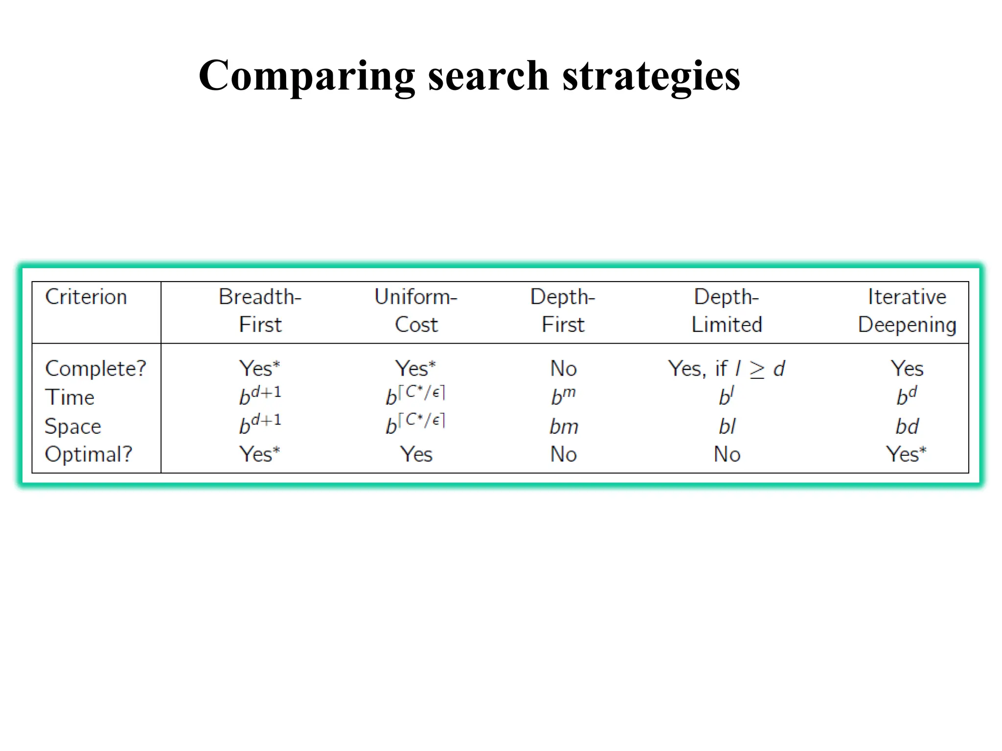
Measuring problem-solving performance
•The evaluation of a search strategy
• Completeness:
• is the strategy guaranteed to find a solution when there is one?
• Optimality:
• does the strategy find the highest-quality solution when there are
several different solutions?
• Time complexity:
• how long does it take to find a solution?
• Space complexity:
• how much memory is needed to perform the search?
31.
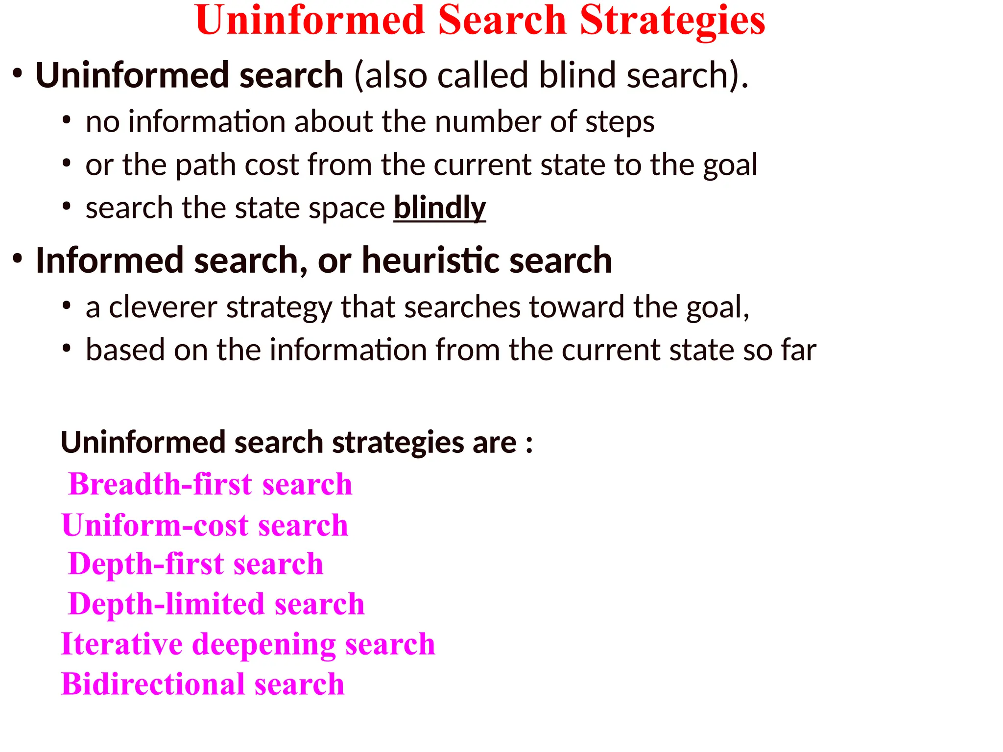
Uninformed Search Strategies
•Uninformed search (also called blind search).
• no information about the number of steps
• or the path cost from the current state to the goal
• search the state space blindly
• Informed search, or heuristic search
• a cleverer strategy that searches toward the goal,
• based on the information from the current state so far
Uninformed search strategies are :
Breadth-first search
Uniform-cost search
Depth-first search
Depth-limited search
Iterative deepening search
Bidirectional search
32.
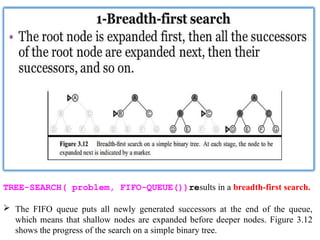
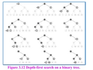
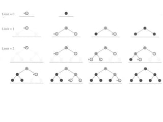
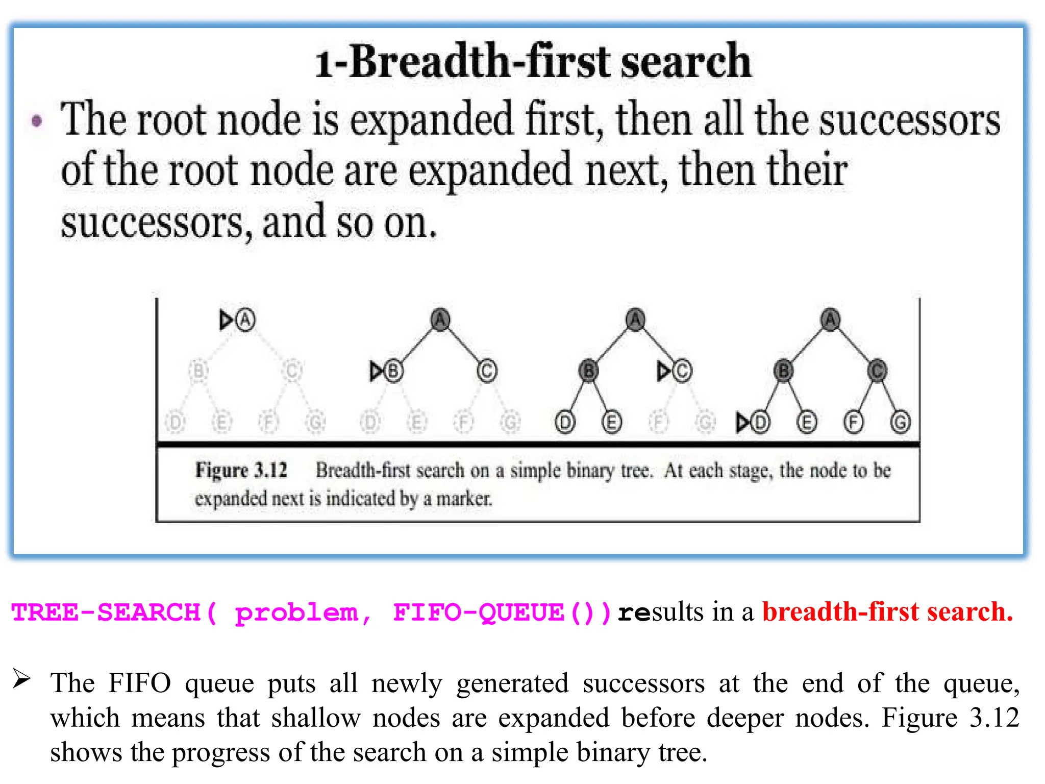
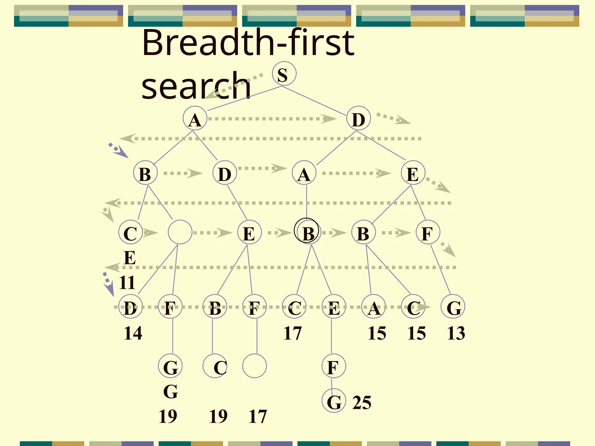
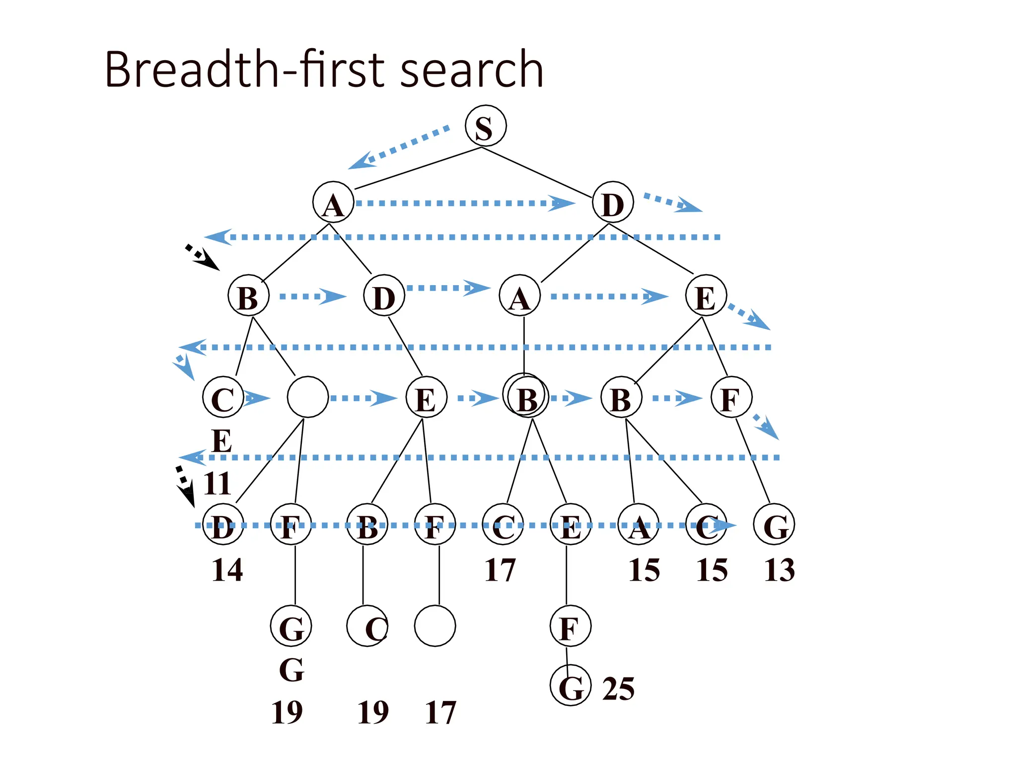
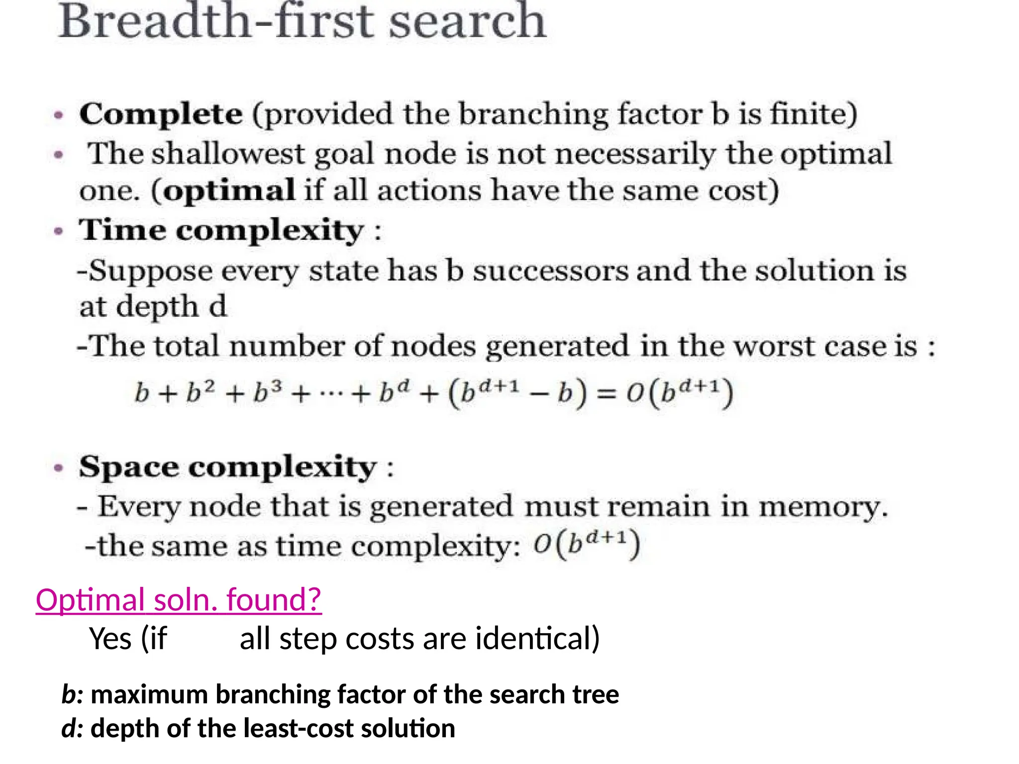
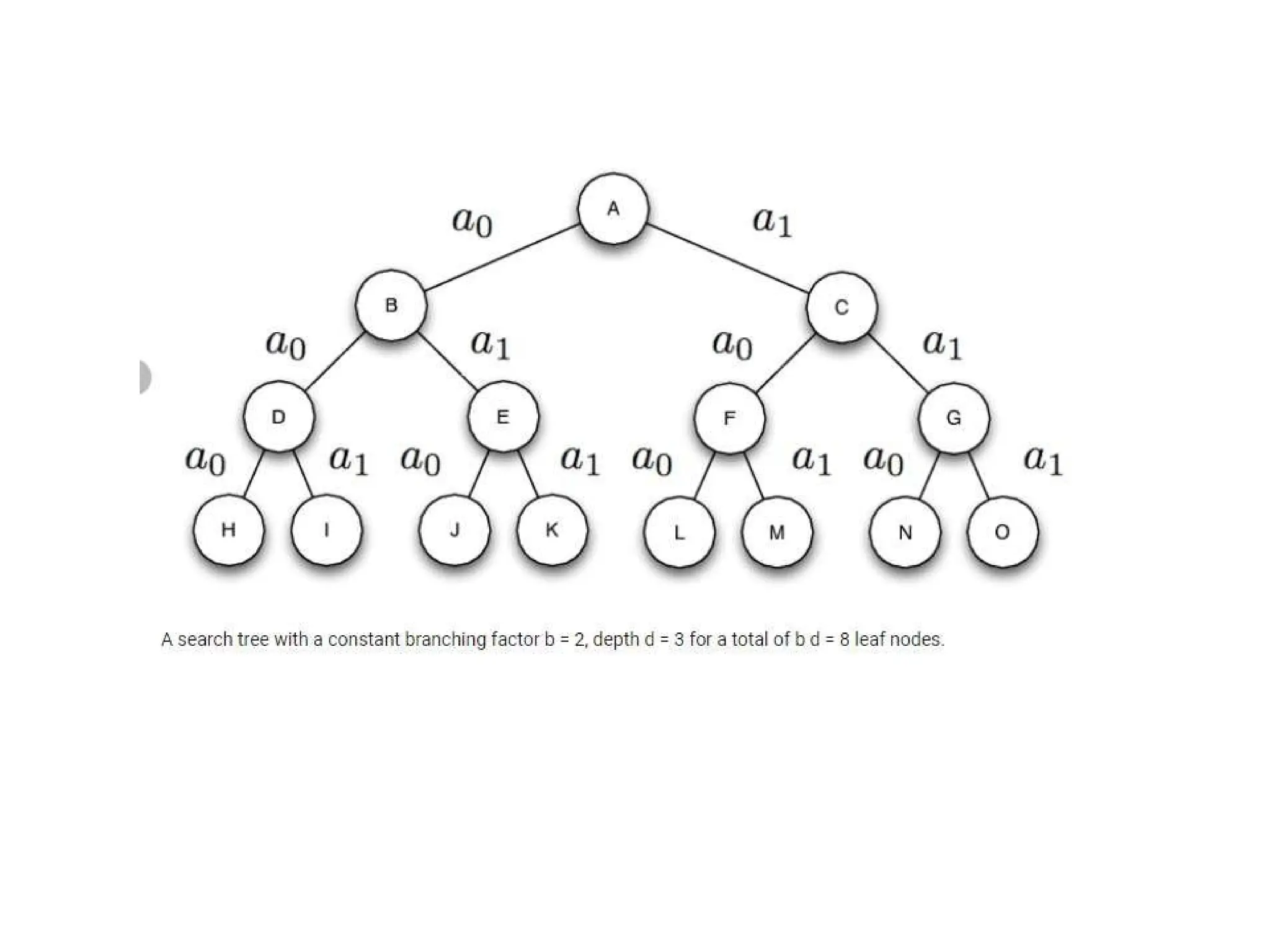
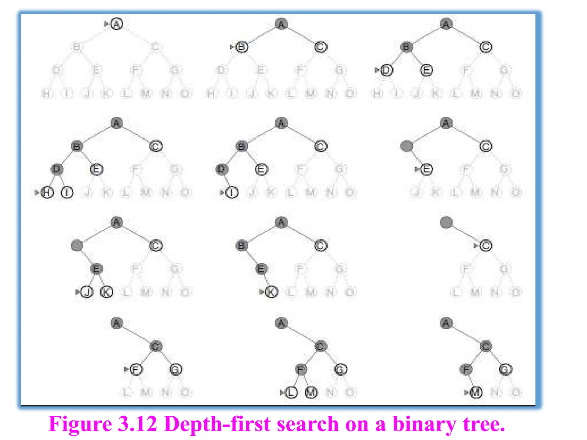
TREE-SEARCH( problem, FIFO-QUEUE())resultsin a breadth-first search.
The FIFO queue puts all newly generated successors at the end of the queue,
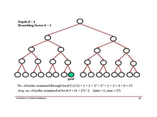
which means that shallow nodes are expanded before deeper nodes. Figure 3.12
shows the progress of the search on a simple binary tree.
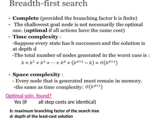
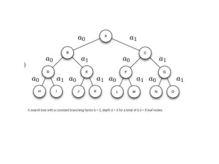
Optimal soln. found?
Yes(if all step costs are identical)
b: maximum branching factor of the search tree
d: depth of the least-cost solution
38.
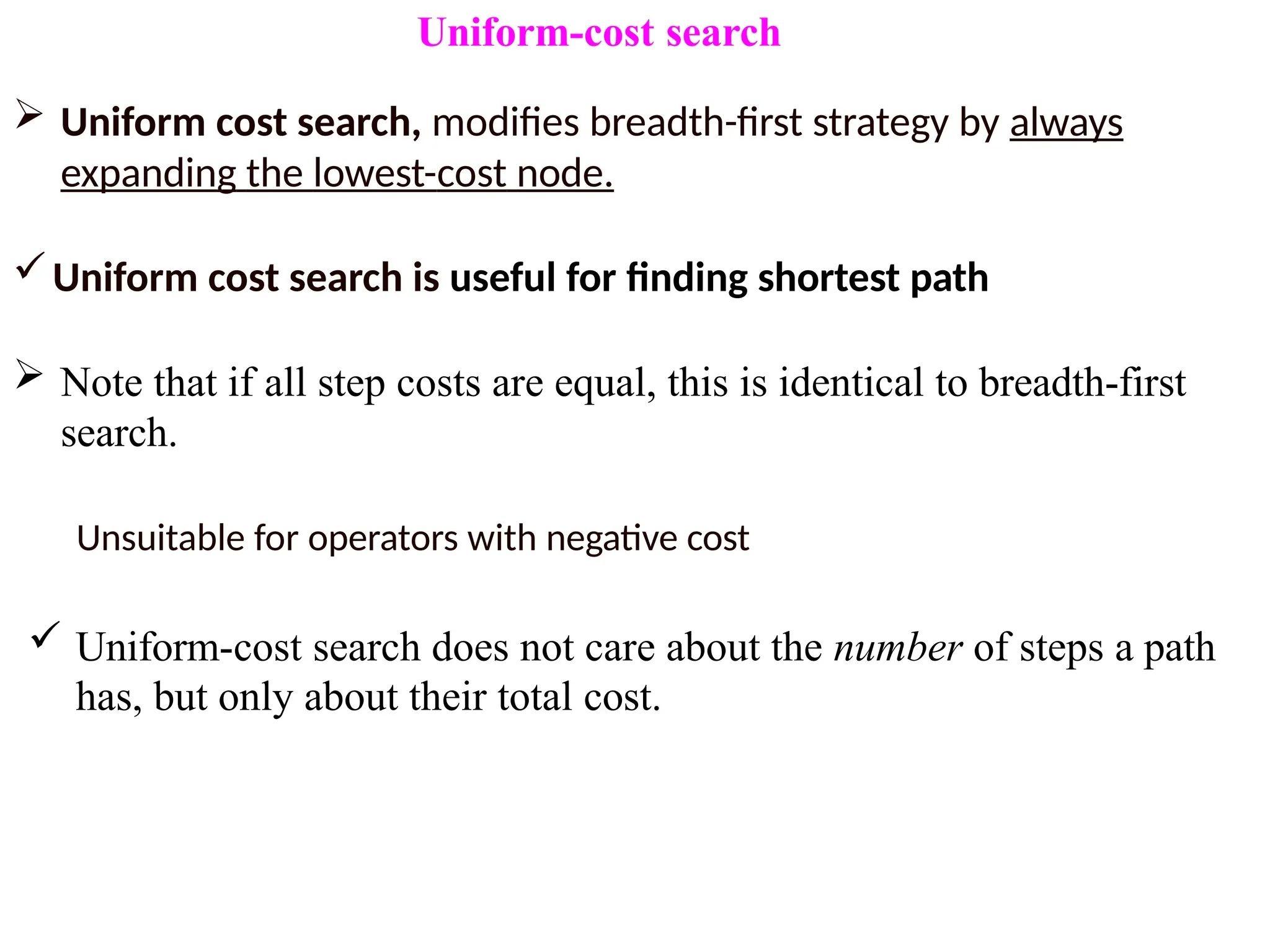
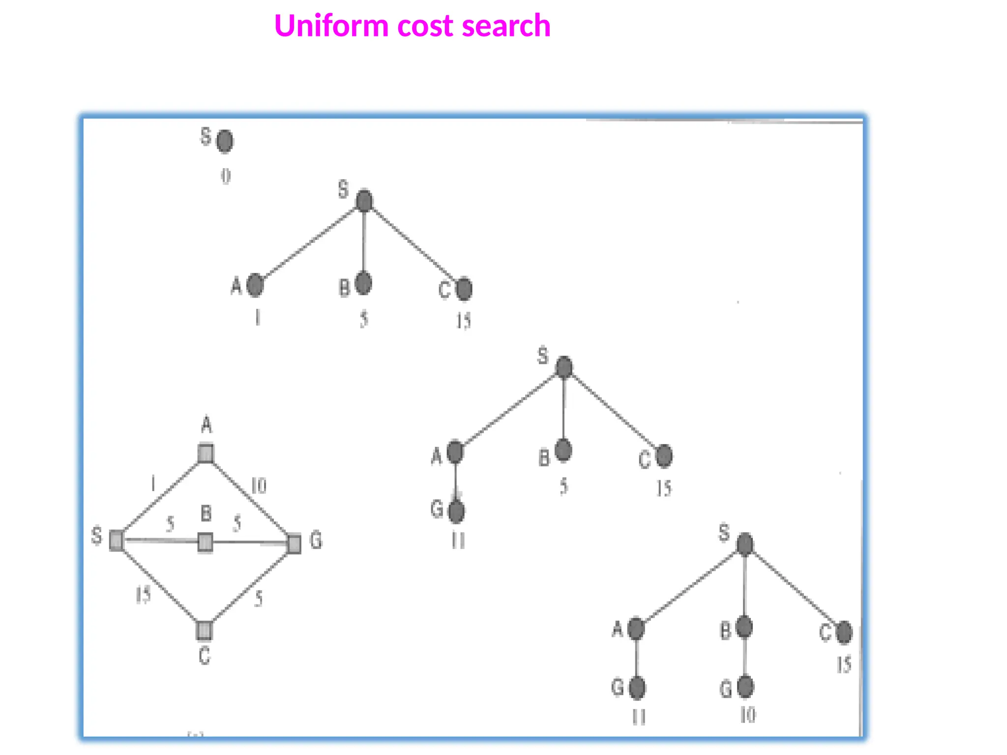
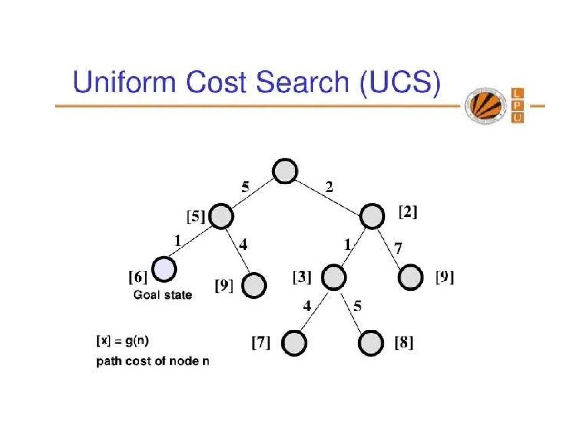
Uniform-cost search
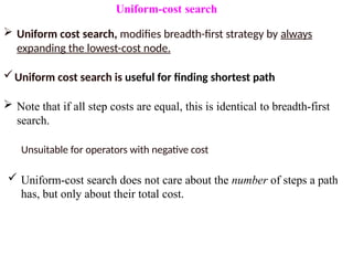
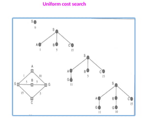
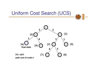
Uniformcost search, modifies breadth-first strategy by always
expanding the lowest-cost node.
Uniform cost search is useful for finding shortest path
Note that if all step costs are equal, this is identical to breadth-first
search.
Unsuitable for operators with negative cost
Uniform-cost search does not care about the number of steps a path
has, but only about their total cost.
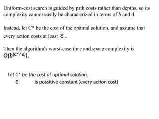
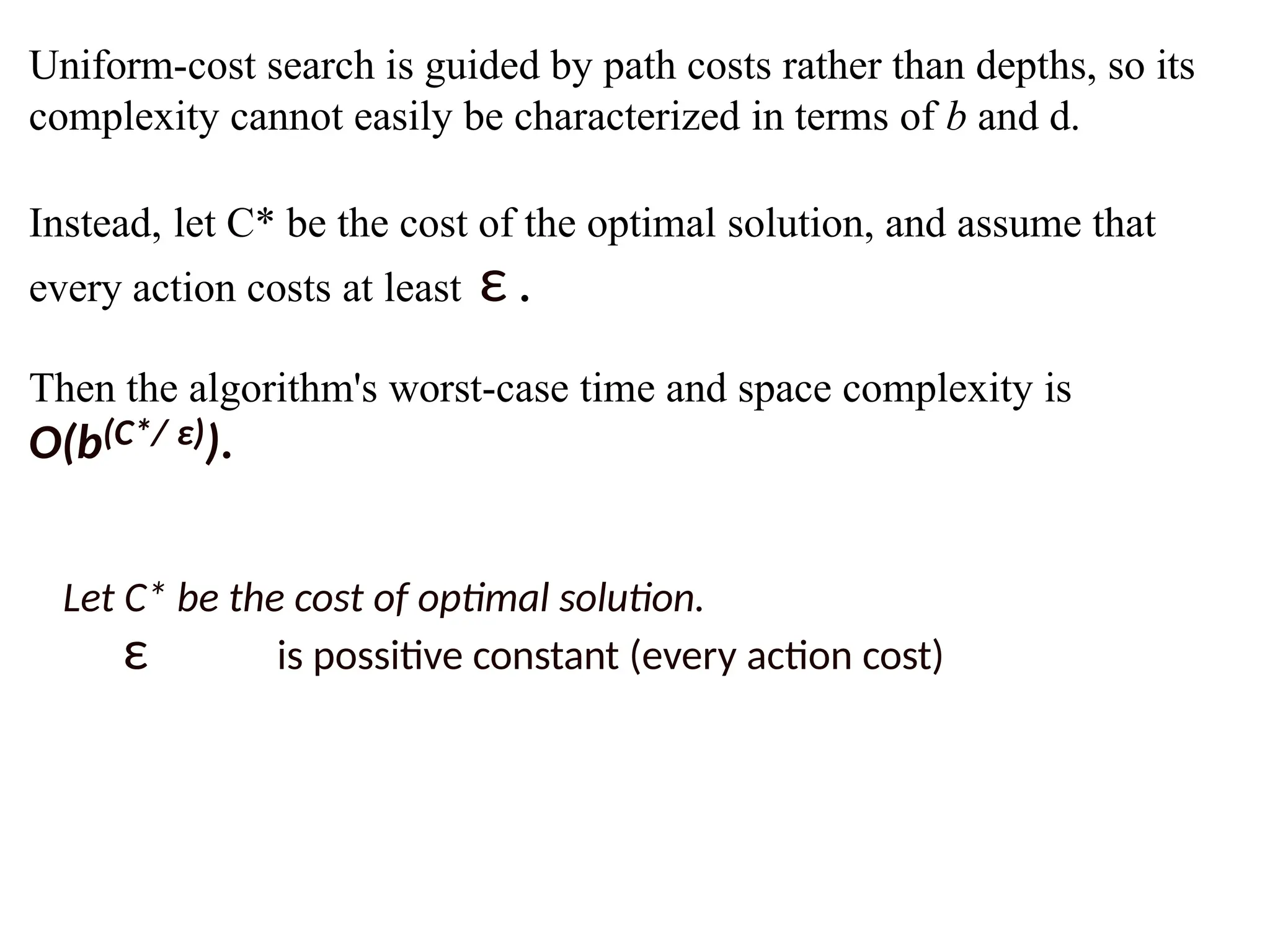
Uniform-cost search isguided by path costs rather than depths, so its
complexity cannot easily be characterized in terms of b and d.
Instead, let C* be the cost of the optimal solution, and assume that
every action costs at least ε .
Then the algorithm's worst-case time and space complexity is
O(b(C*/ ε)).
Let C* be the cost of optimal solution.
ε is possitive constant (every action cost)
42.
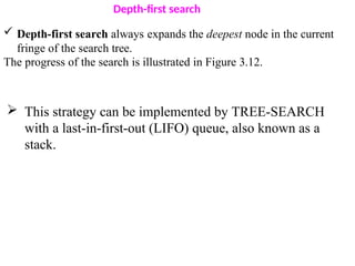
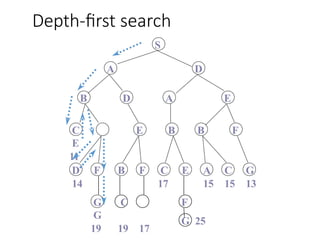
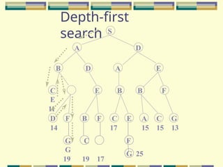
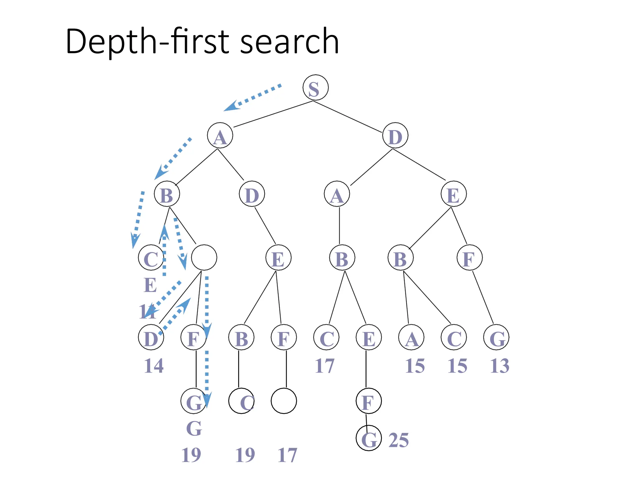
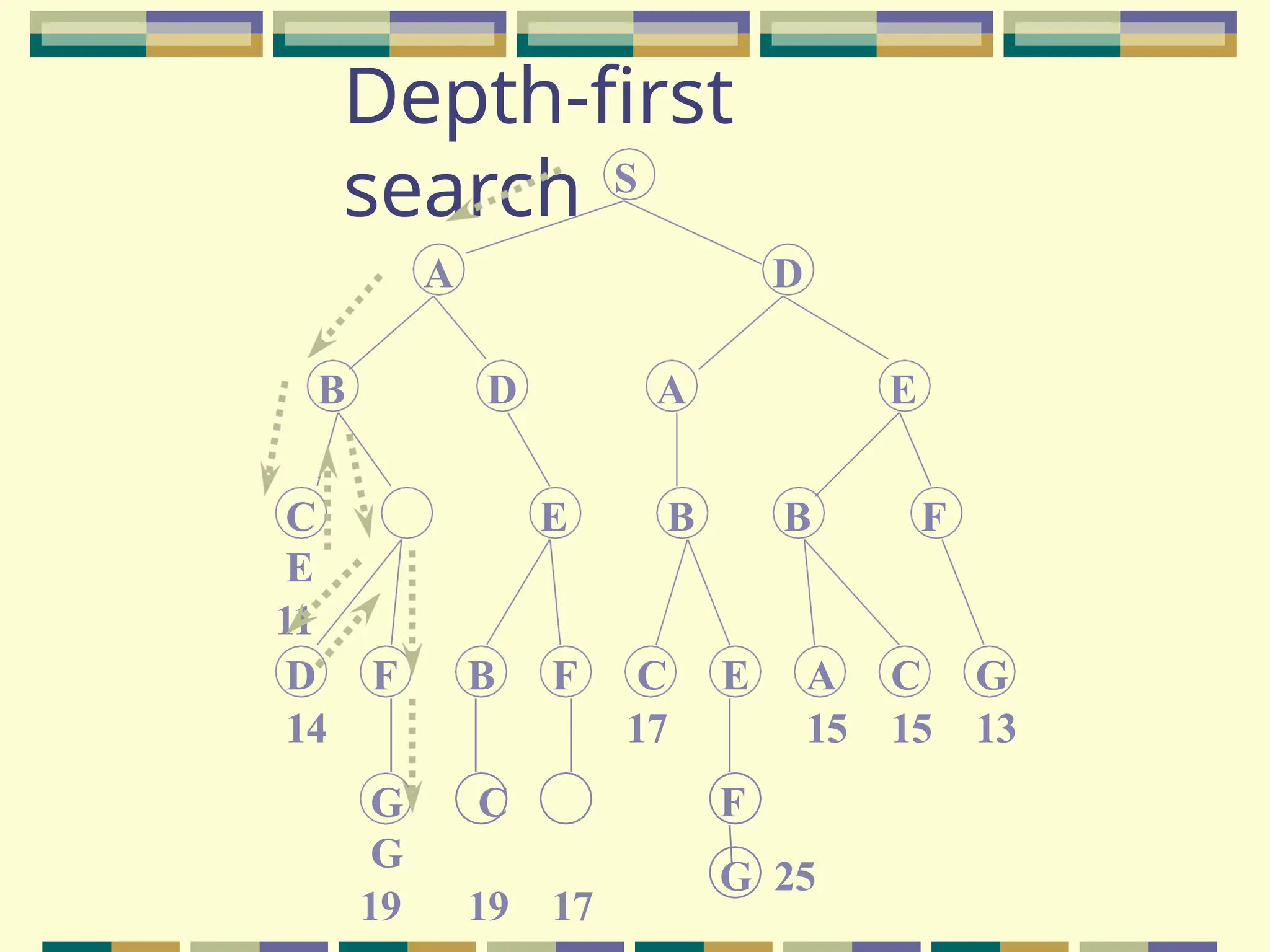
Depth-first search
Depth-firstsearch always expands the deepest node in the current
fringe of the search tree.
The progress of the search is illustrated in Figure 3.12.
This strategy can be implemented by TREE-SEARCH
with a last-in-first-out (LIFO) queue, also known as a
stack.
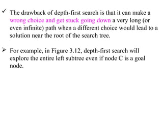
The drawbackof depth-first search is that it can make a
wrong choice and get stuck going down a very long (or
even infinite) path when a different choice would lead to a
solution near the root of the search tree.
For example, in Figure 3.12, depth-first search will
explore the entire left subtree even if node C is a goal
node.
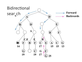
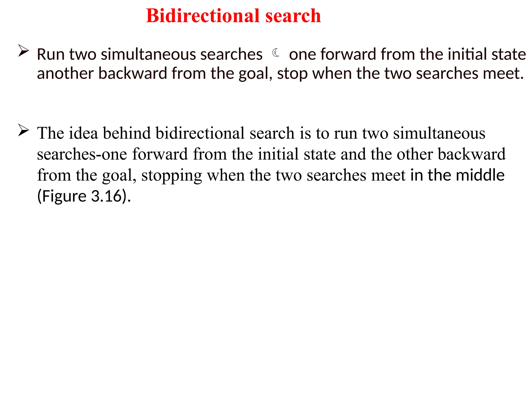
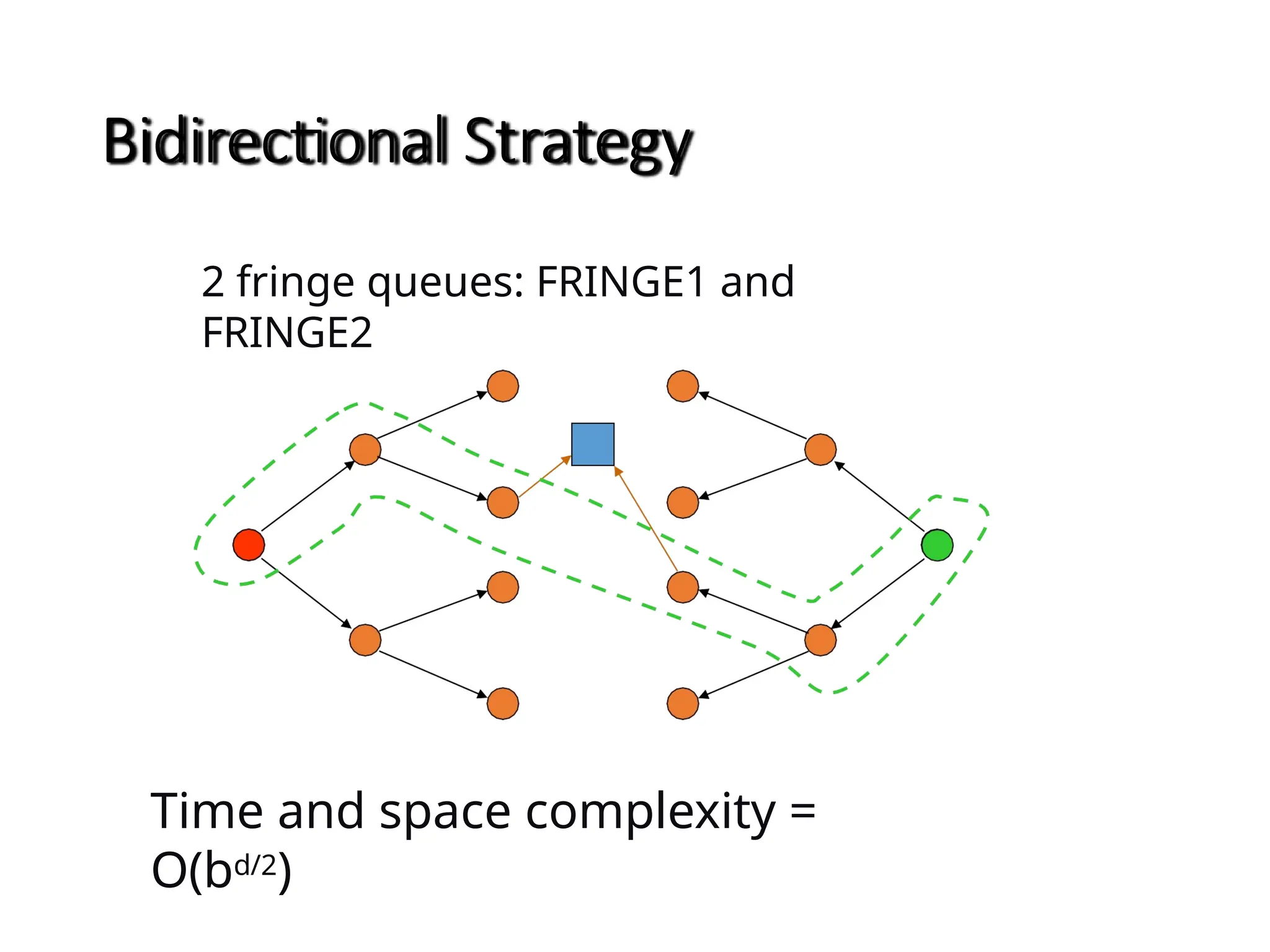
Bidirectional search
Runtwo simultaneous searches one forward from the initial state
another backward from the goal, stop when the two searches meet.
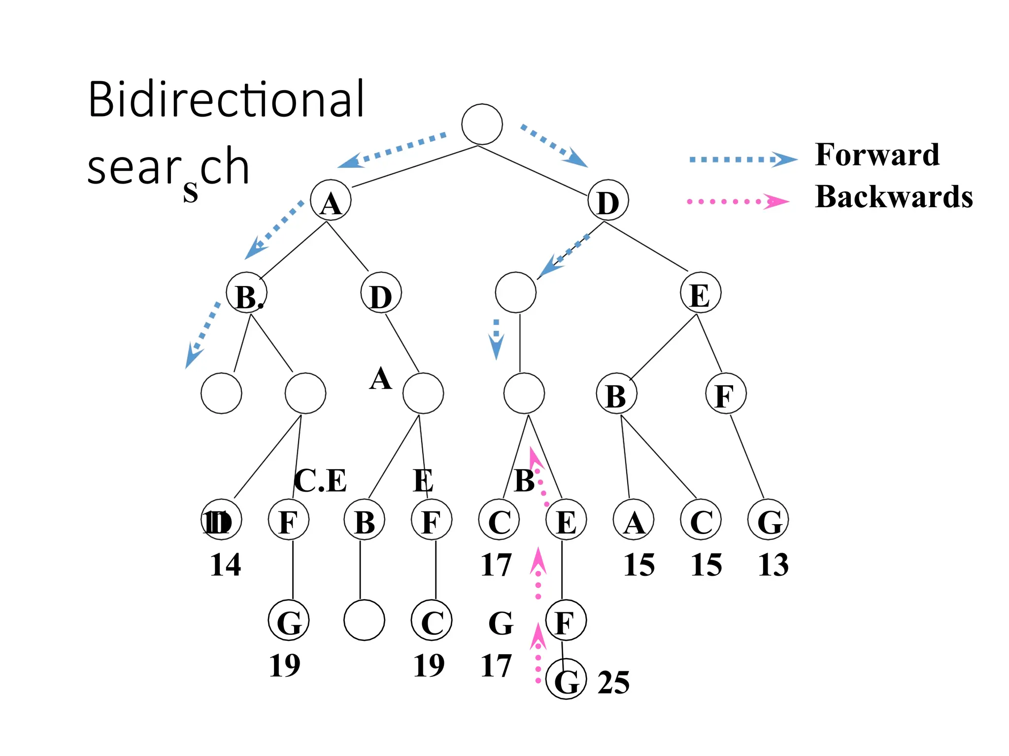
The idea behind bidirectional search is to run two simultaneous
searches-one forward from the initial state and the other backward
from the goal, stopping when the two searches meet in the middle
(Figure 3.16).
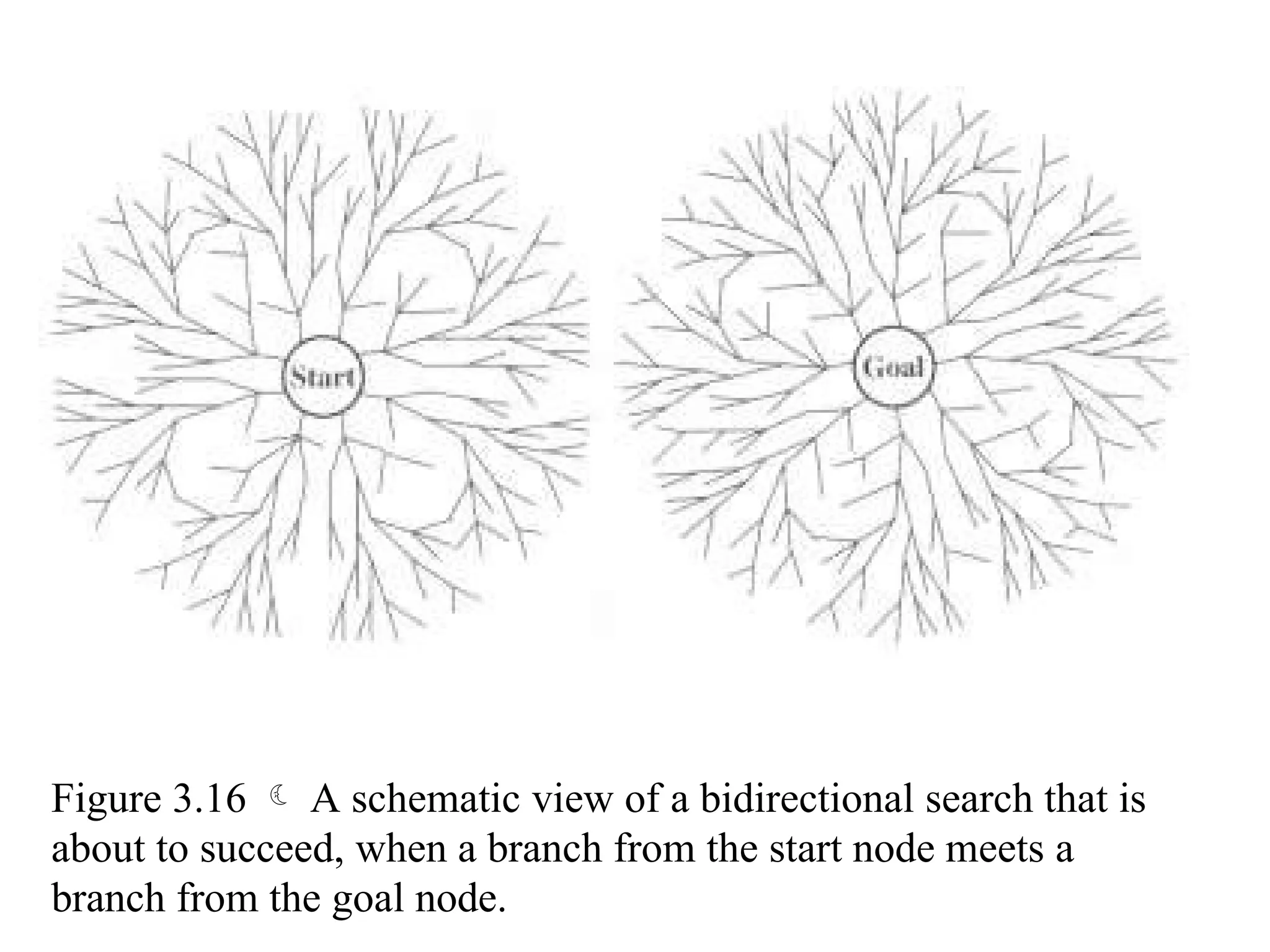
Figure 3.16 A schematic view of a bidirectional search that is
about to succeed, when a branch from the start node meets a
branch from the goal node.
51.
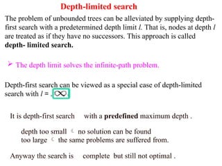
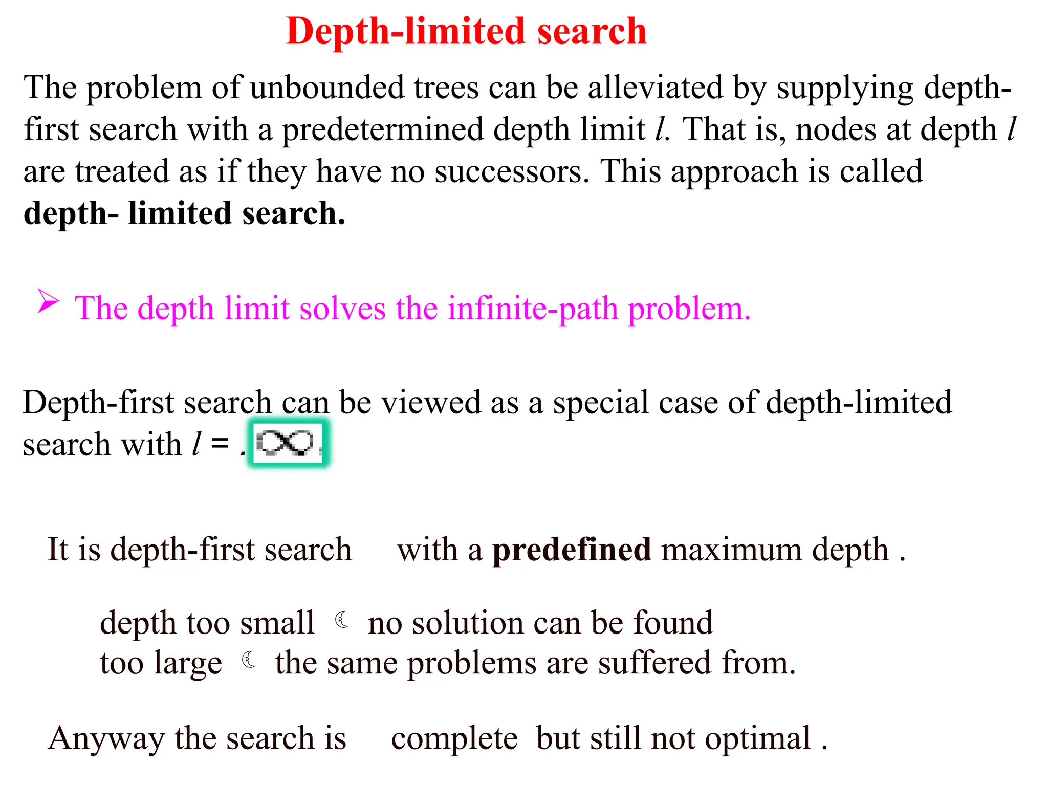
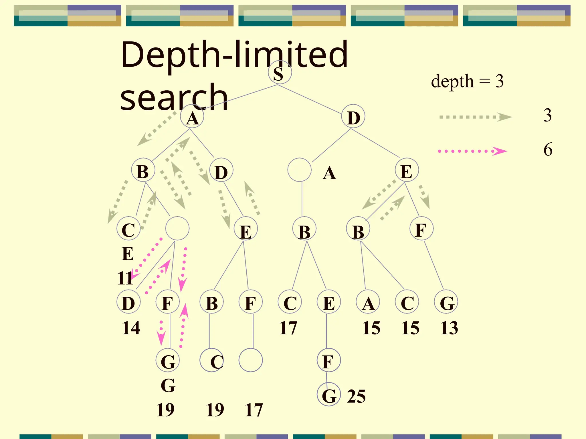
Depth-limited search
The problemof unbounded trees can be alleviated by supplying depth-
first search with a predetermined depth limit l. That is, nodes at depth l
are treated as if they have no successors. This approach is called
depth- limited search.
The depth limit solves the infinite-path problem.
Depth-first search can be viewed as a special case of depth-limited
search with l = .
It is depth-first search with a predefined maximum depth .
depth too small no solution can be found
too large the same problems are suffered from.
Anyway the search is complete but still not optimal .
52.
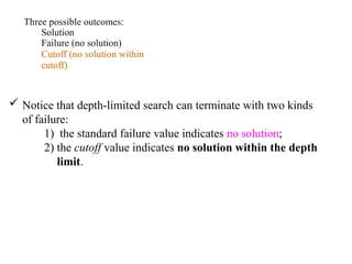
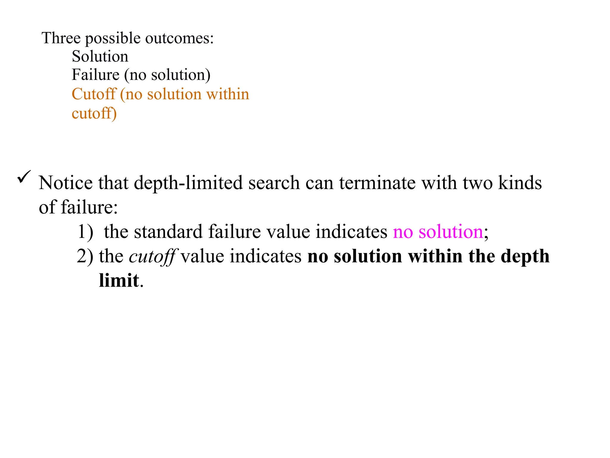
Three possible outcomes:
Solution
Failure(no solution)
Cutoff (no solution within
cutoff)
Notice that depth-limited search can terminate with two kinds
of failure:
1) the standard failure value indicates no solution;
2) the cutoff value indicates no solution within the depth
limit.
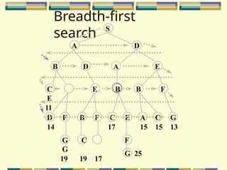
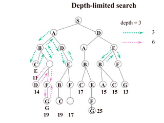
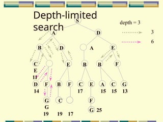
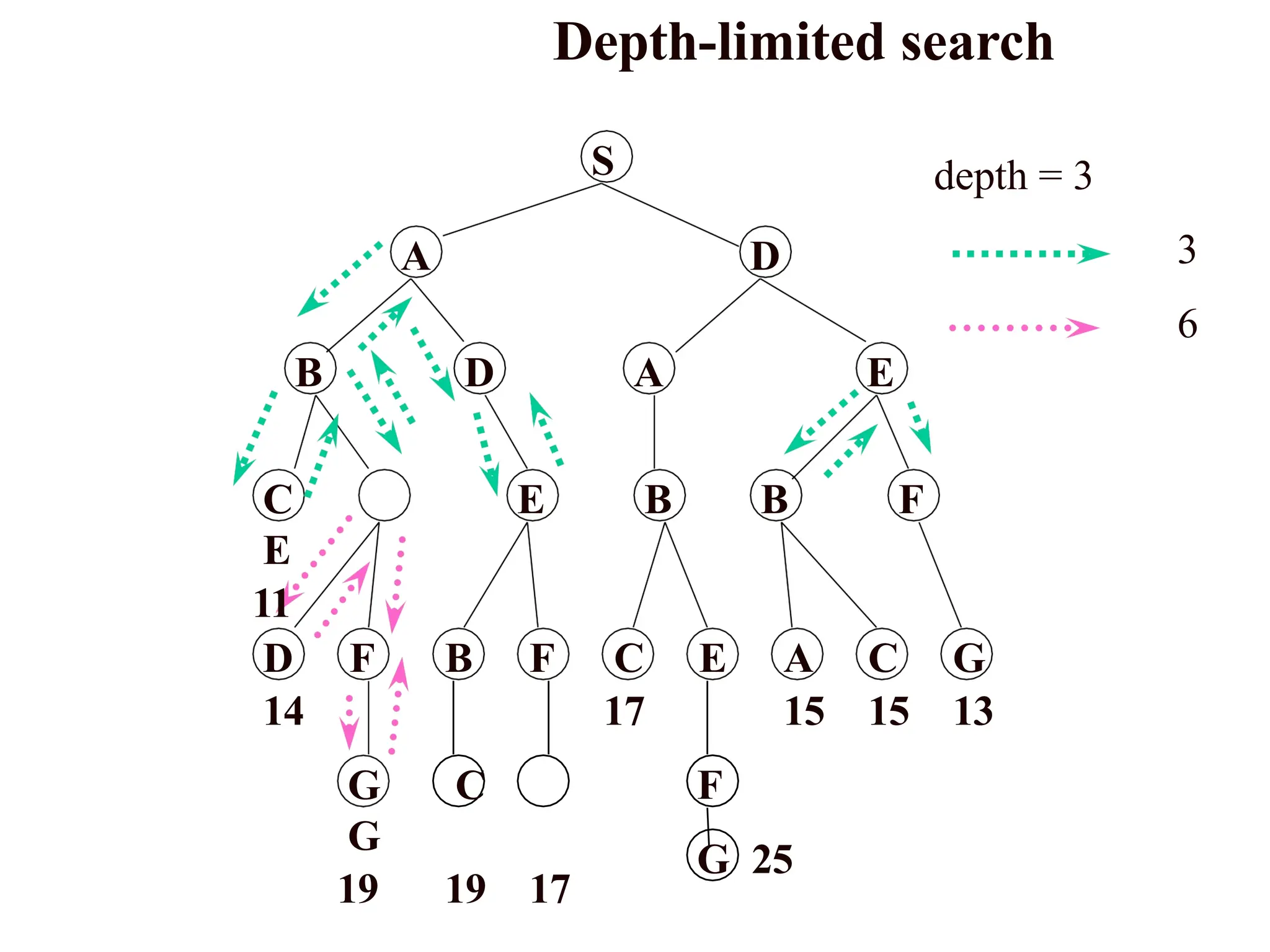
54.
Depth-limited search
S
A D
BD A E
E B B F
G C
G
19 19 17
D F B F C E A C G
14 17 15 15 13
F
G 25
C
E
11
depth = 3
3
6
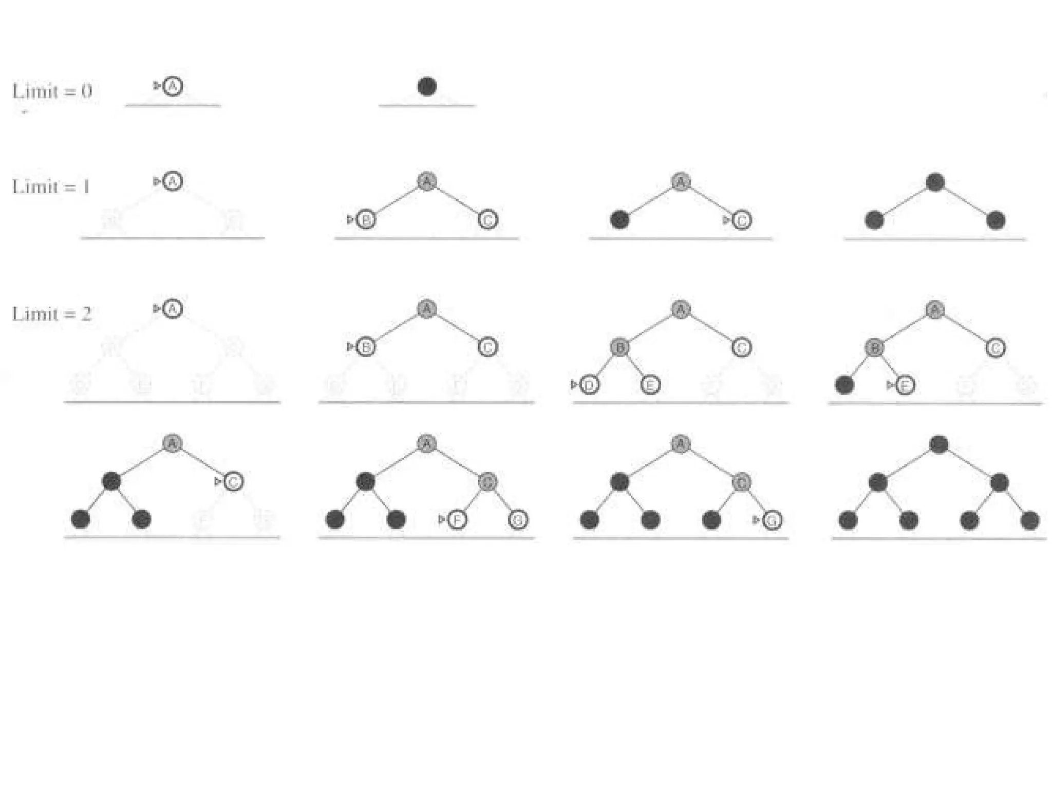
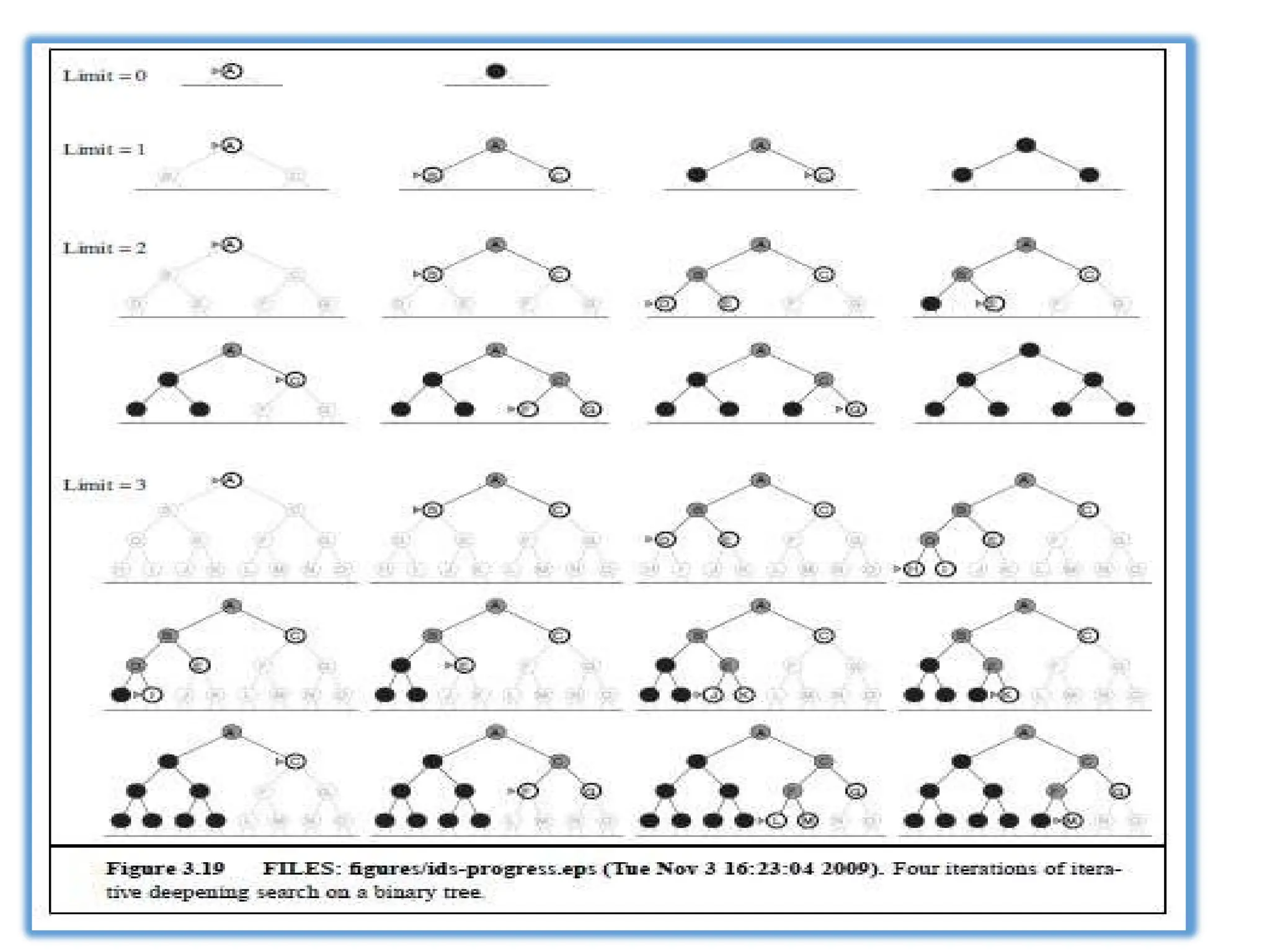
Iterative deepening searchor iterative deepening depth-first search
Iterative deepening combines the benefits of depth-first and breadth-
first search.
In general, iterative deepening is the preferred uninformed search
method when there is a large search space and the depth of the
solution is not known.
59.
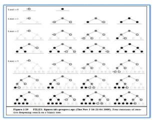
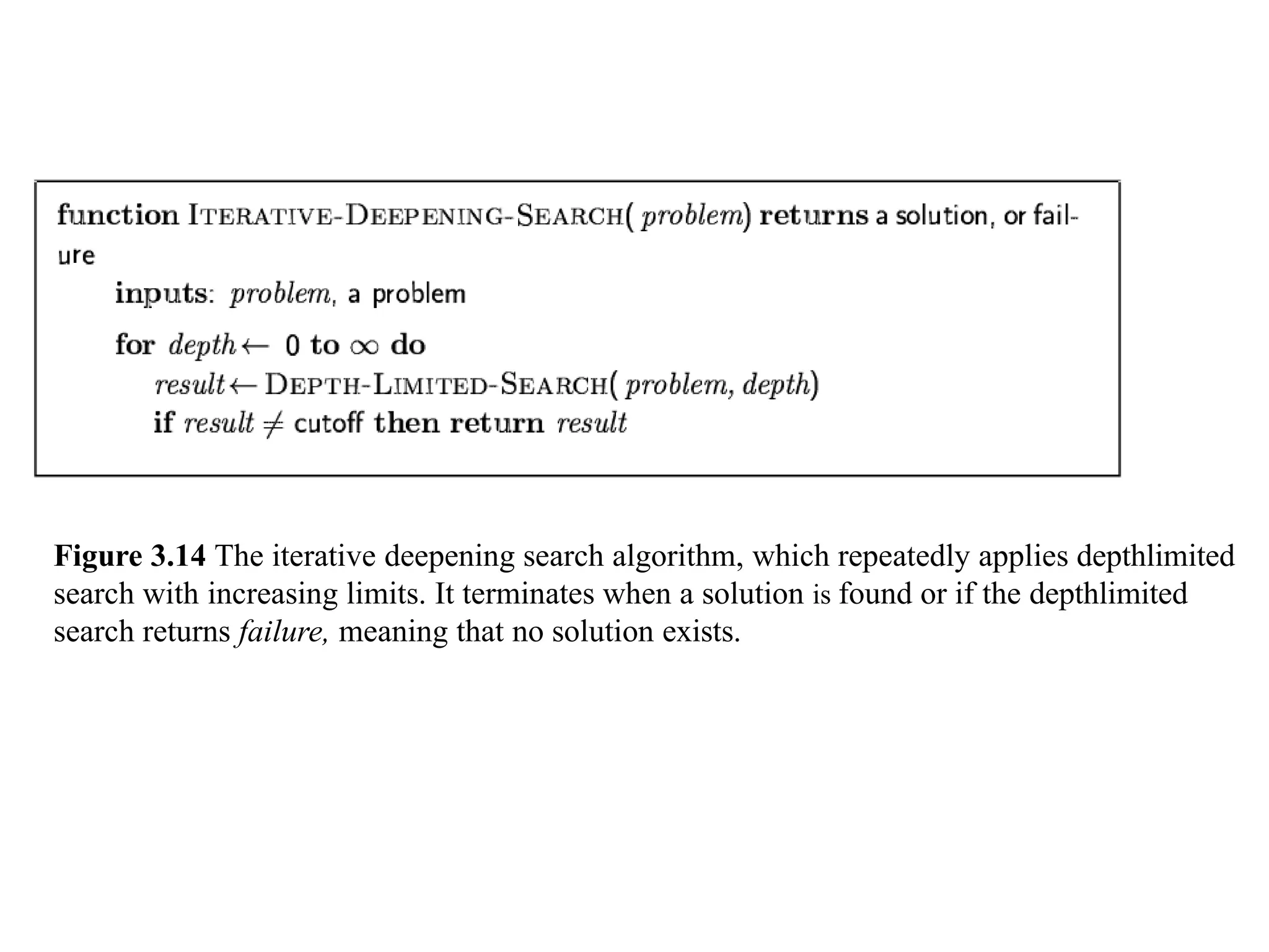
Figure 3.14 Theiterative deepening search algorithm, which repeatedly applies depthlimited
search with increasing limits. It terminates when a solution is found or if the depthlimited
search returns failure, meaning that no solution exists.
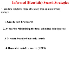
Informed (Heuristic) SearchStrategies
can find solutions more efficiently than an uninformed
strategy.
1. Greedy best-first search
2. A* search: Minimizing the total estimated solution cost
3. Memory-bounded heuristic search
4. Recursive best-first search (RBFS)
64.
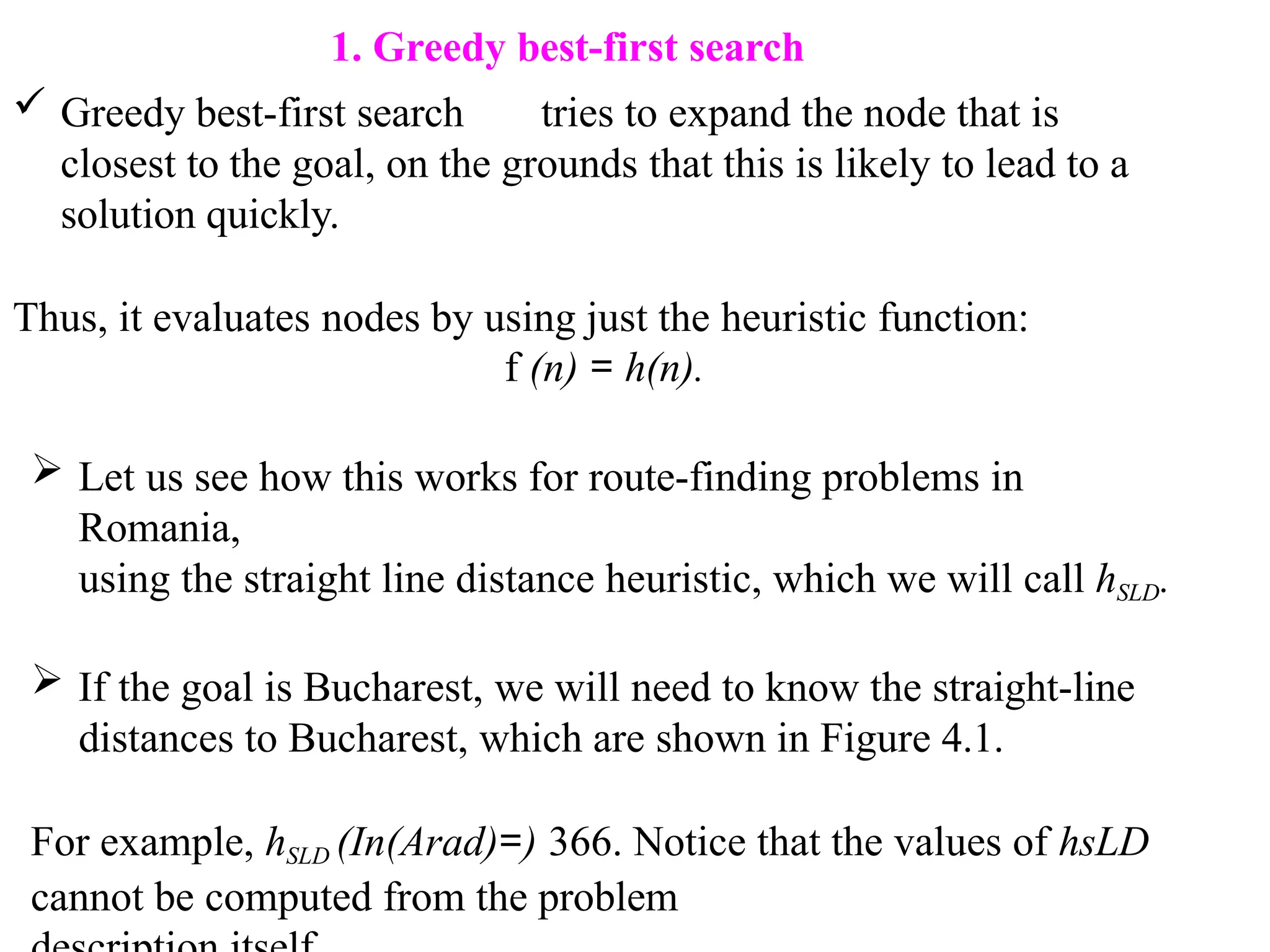
1. Greedy best-firstsearch
Greedy best-first search tries to expand the node that is
closest to the goal, on the grounds that this is likely to lead to a
solution quickly.
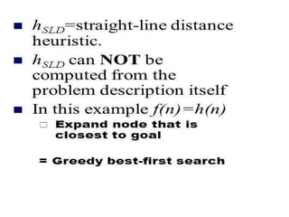
Thus, it evaluates nodes by using just the heuristic function:
f (n) = h(n).
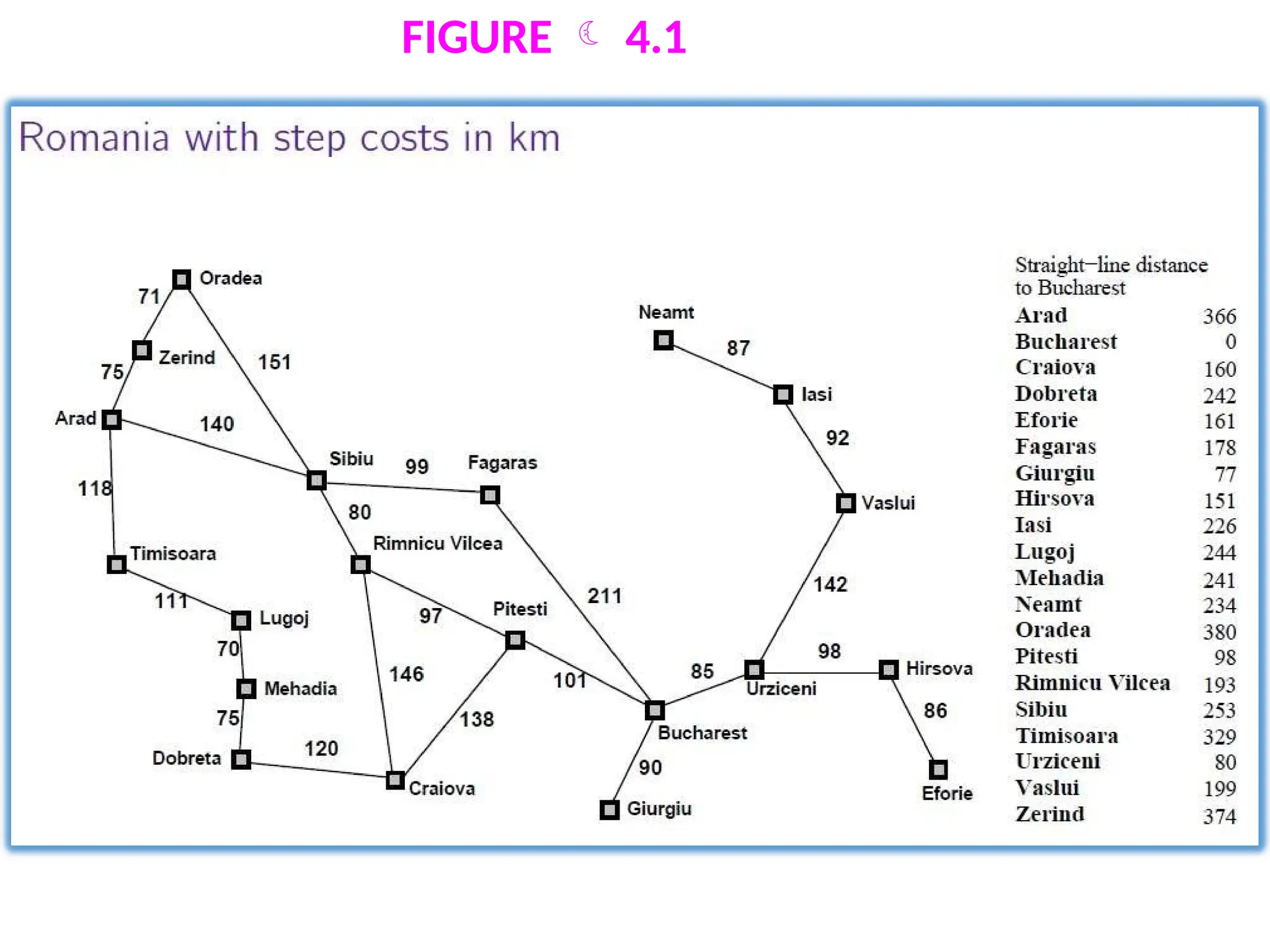
Let us see how this works for route-finding problems in
Romania,
using the straight line distance heuristic, which we will call hSLD.
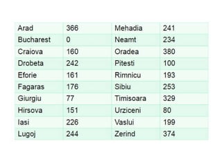
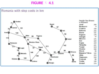
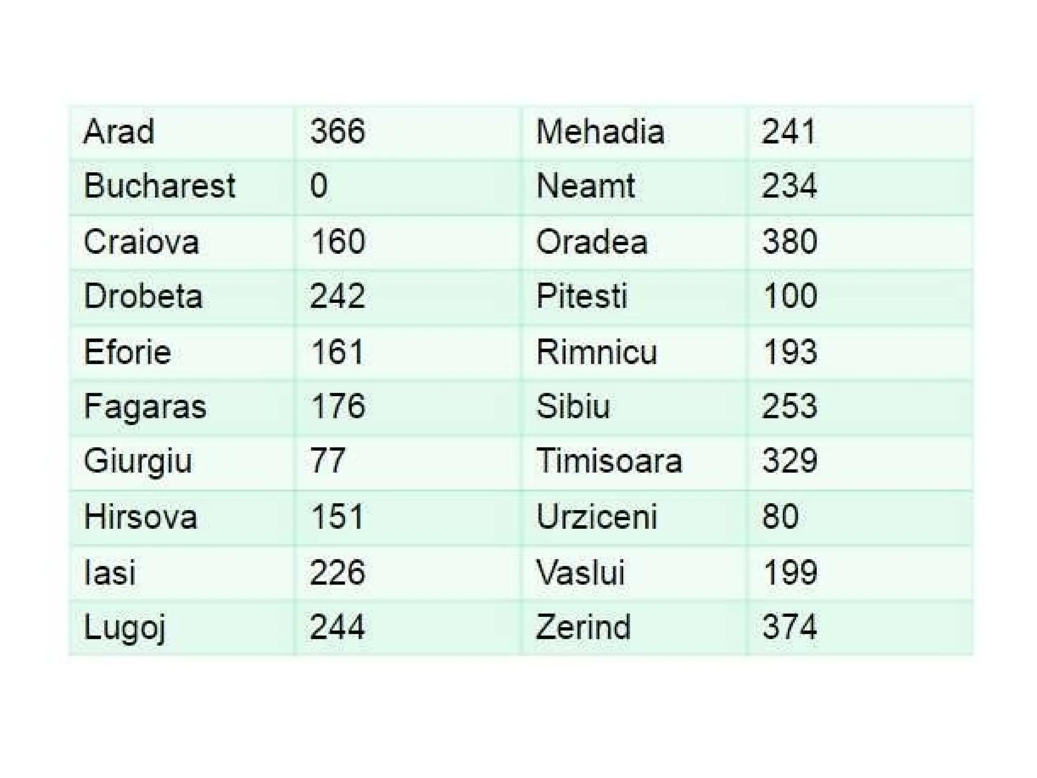
If the goal is Bucharest, we will need to know the straight-line
distances to Bucharest, which are shown in Figure 4.1.
For example, hSLD (In(Arad)=) 366. Notice that the values of hsLD
cannot be computed from the problem
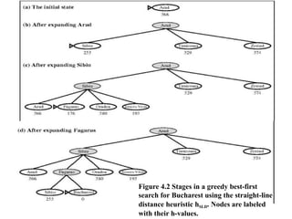
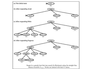
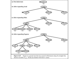
Figure 4.2 Stagesin a greedy best-first
search for Bucharest using the straight-line
distance heuristic hSLD. Nodes are labeled
with their h-values.
72.
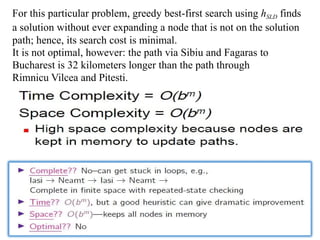
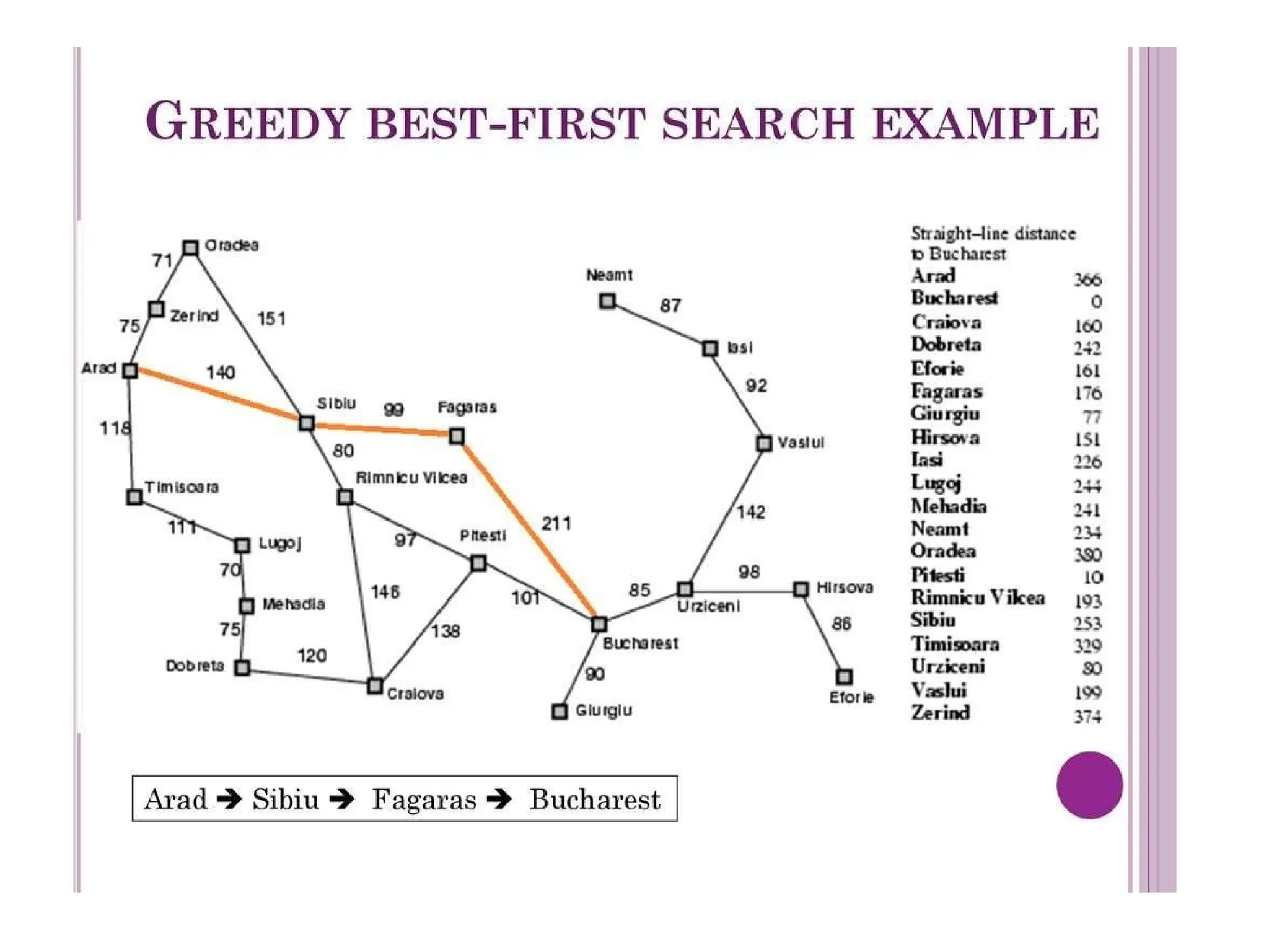
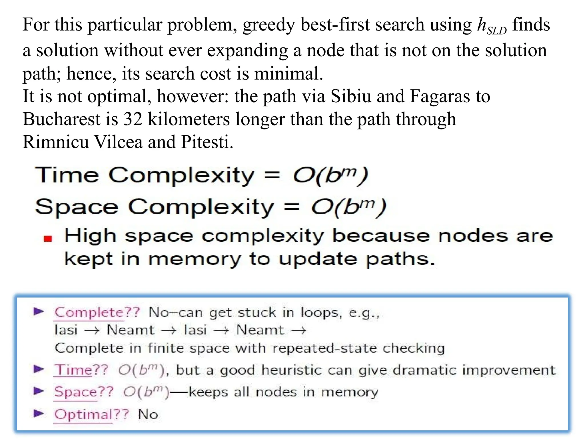
For this particularproblem, greedy best-first search using hSLD finds
a solution without ever expanding a node that is not on the solution
path; hence, its search cost is minimal.
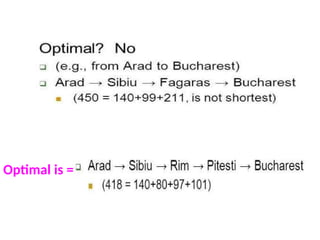
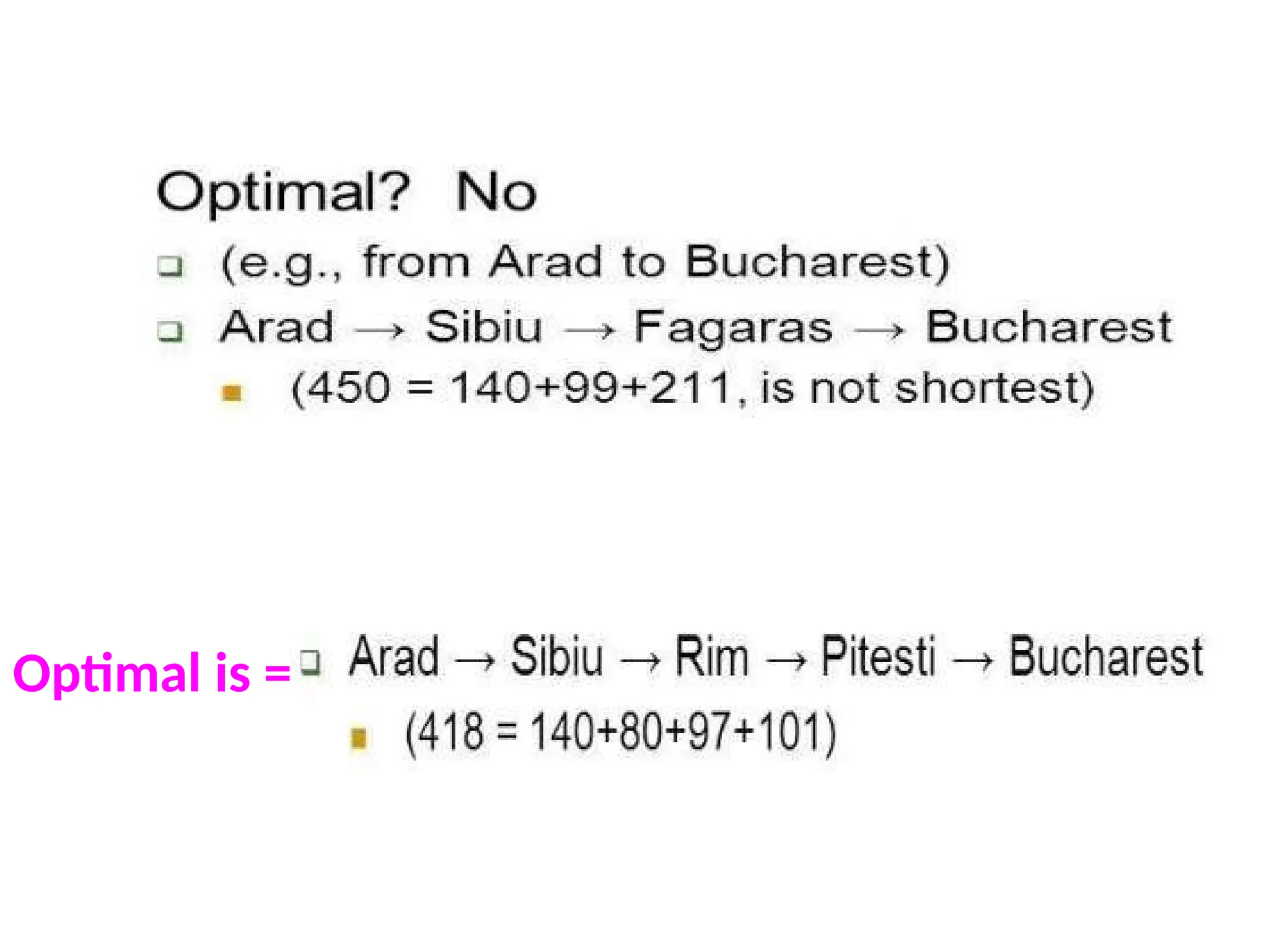
It is not optimal, however: the path via Sibiu and Fagaras to
Bucharest is 32 kilometers longer than the path through
Rimnicu Vilcea and Pitesti.
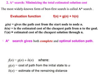
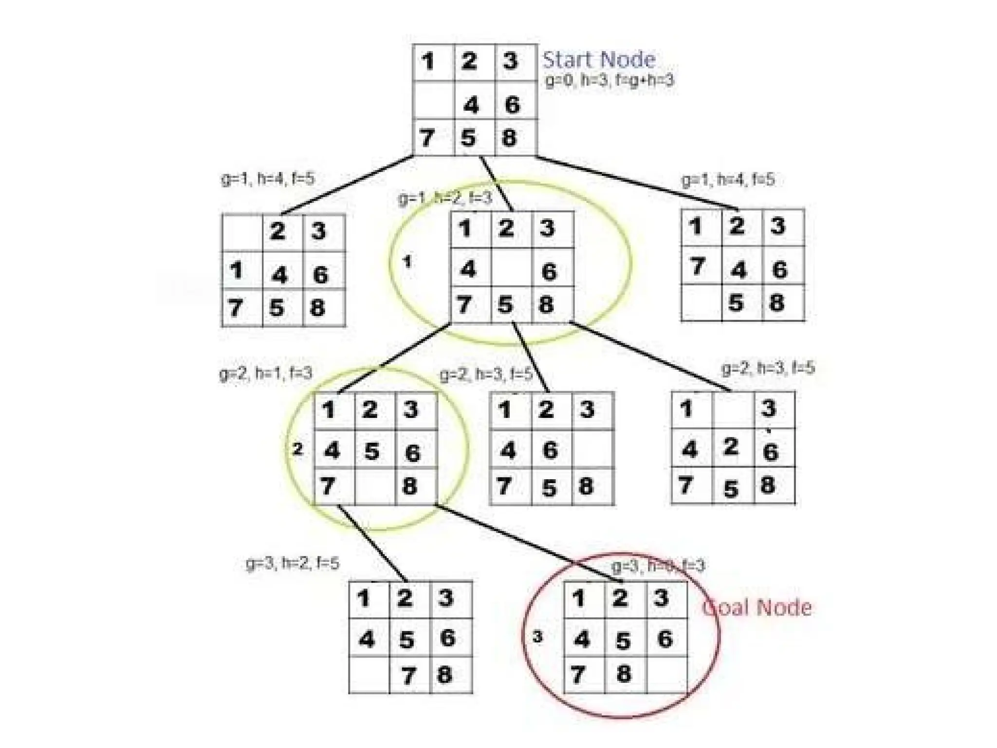
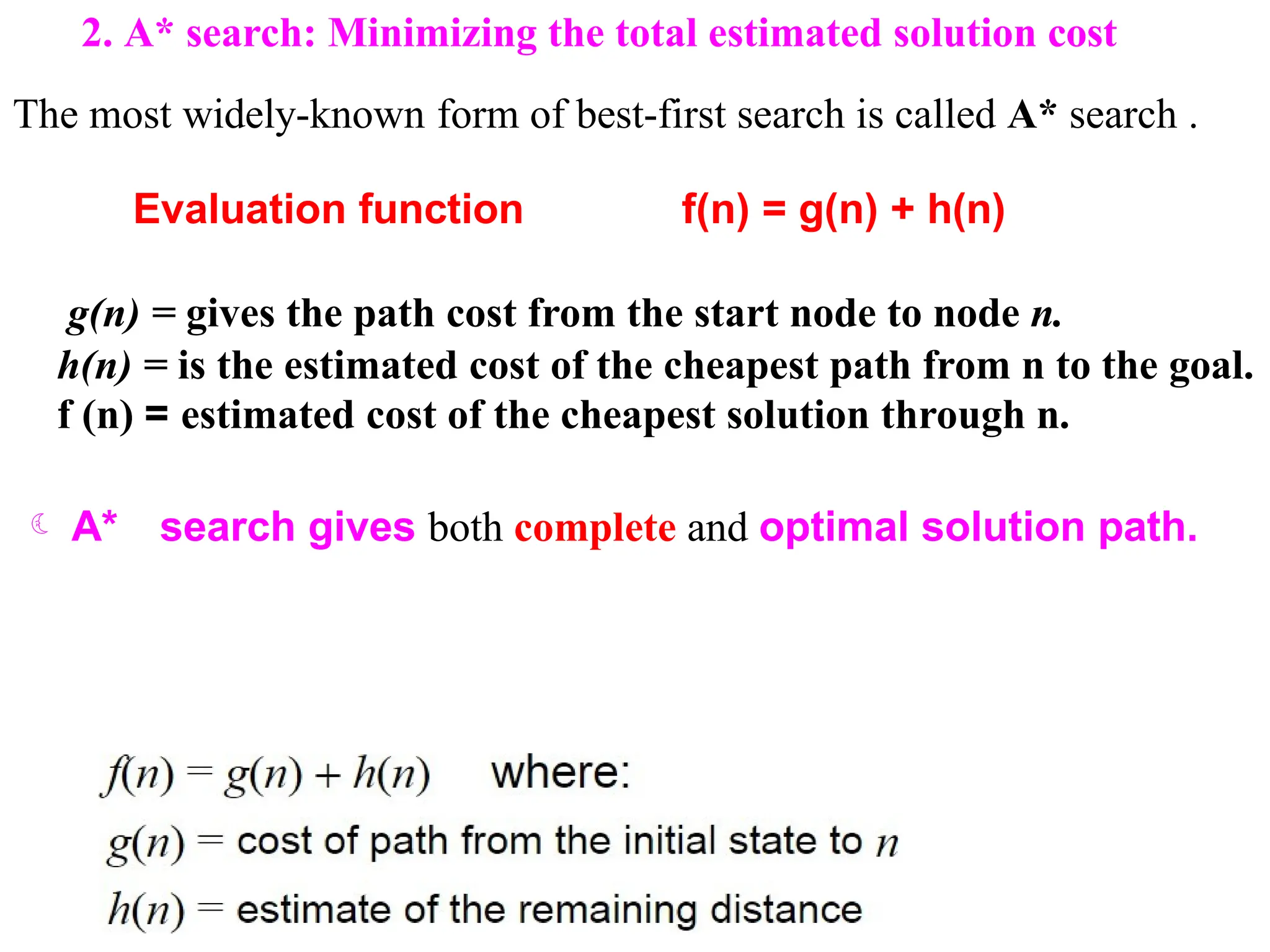
2. A* search:Minimizing the total estimated solution cost
The most widely-known form of best-first search is called A* search .
Evaluation function f(n) = g(n) + h(n)
g(n) = gives the path cost from the start node to node n.
h(n) = is the estimated cost of the cheapest path from n to the goal.
f (n) = estimated cost of the cheapest solution through n.
A* search gives both complete and optimal solution path.
75.
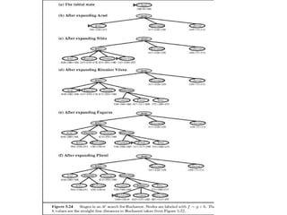
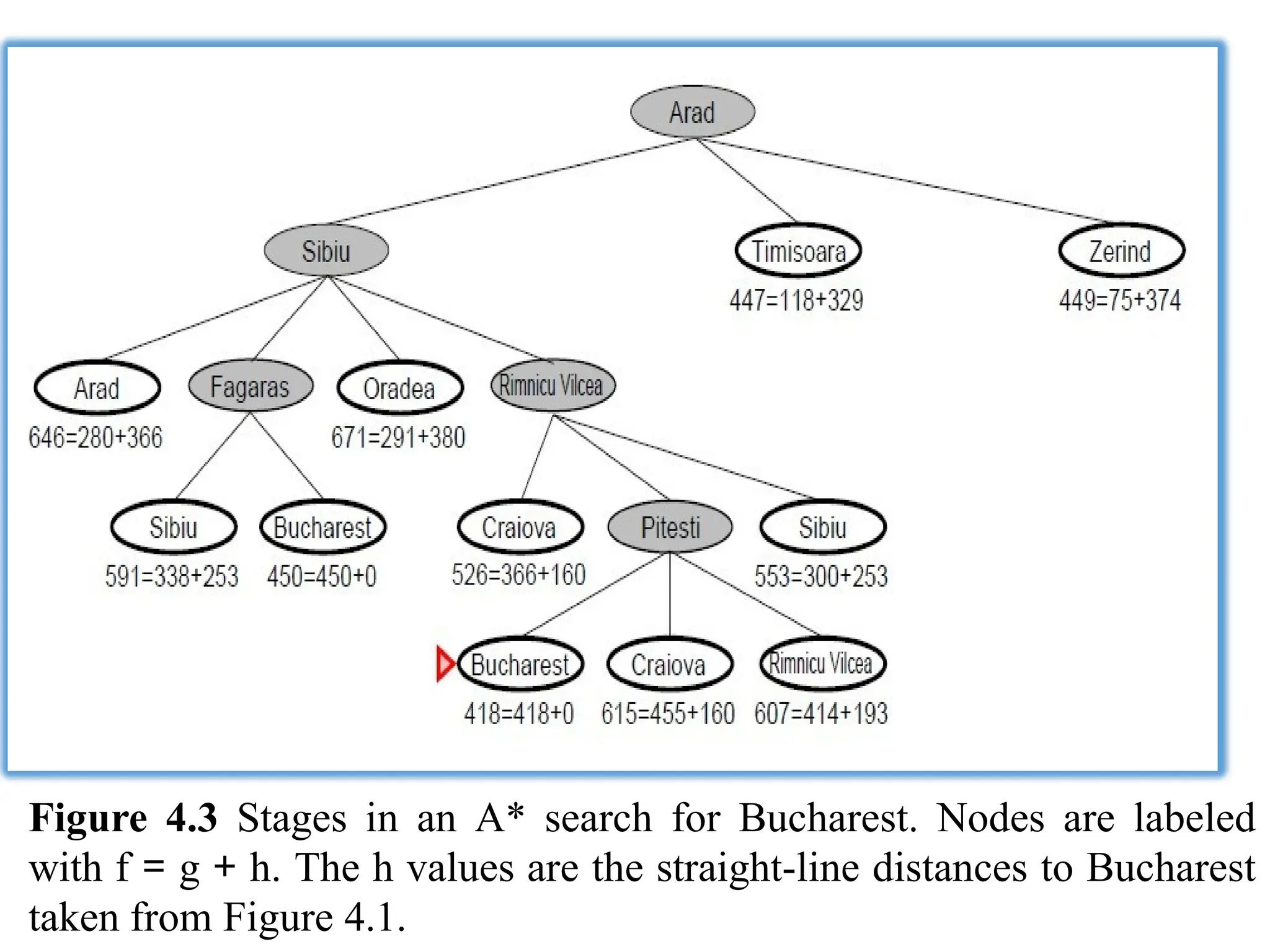
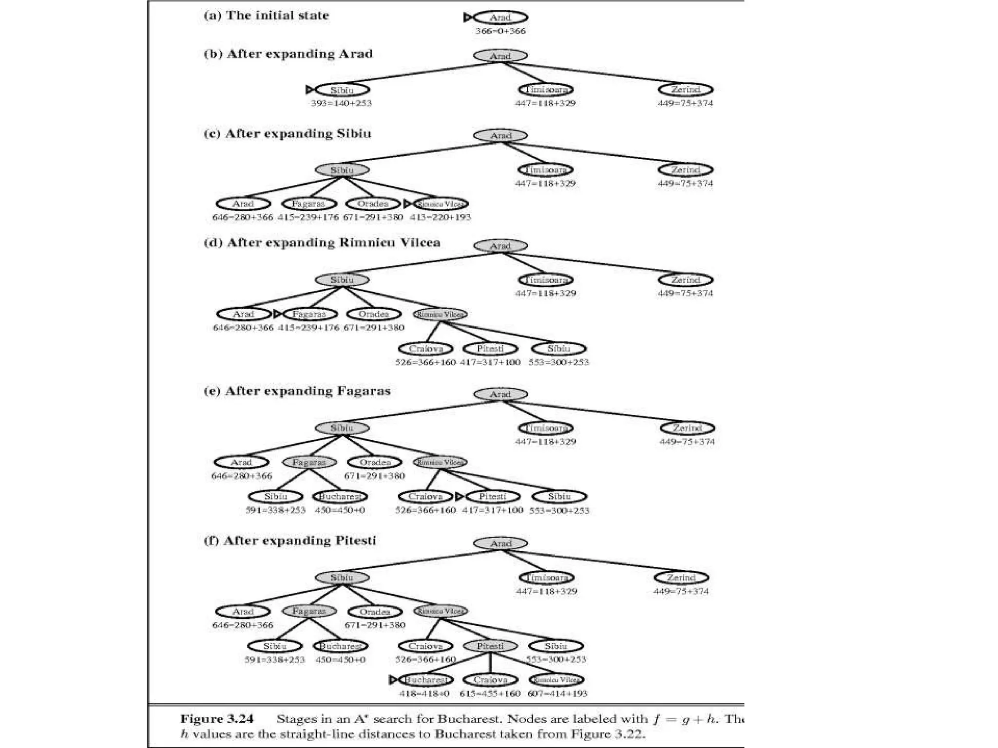
Figure 4.3 Stagesin an A* search for Bucharest. Nodes are labeled
with f = g + h. The h values are the straight-line distances to Bucharest
taken from Figure 4.1.
77.
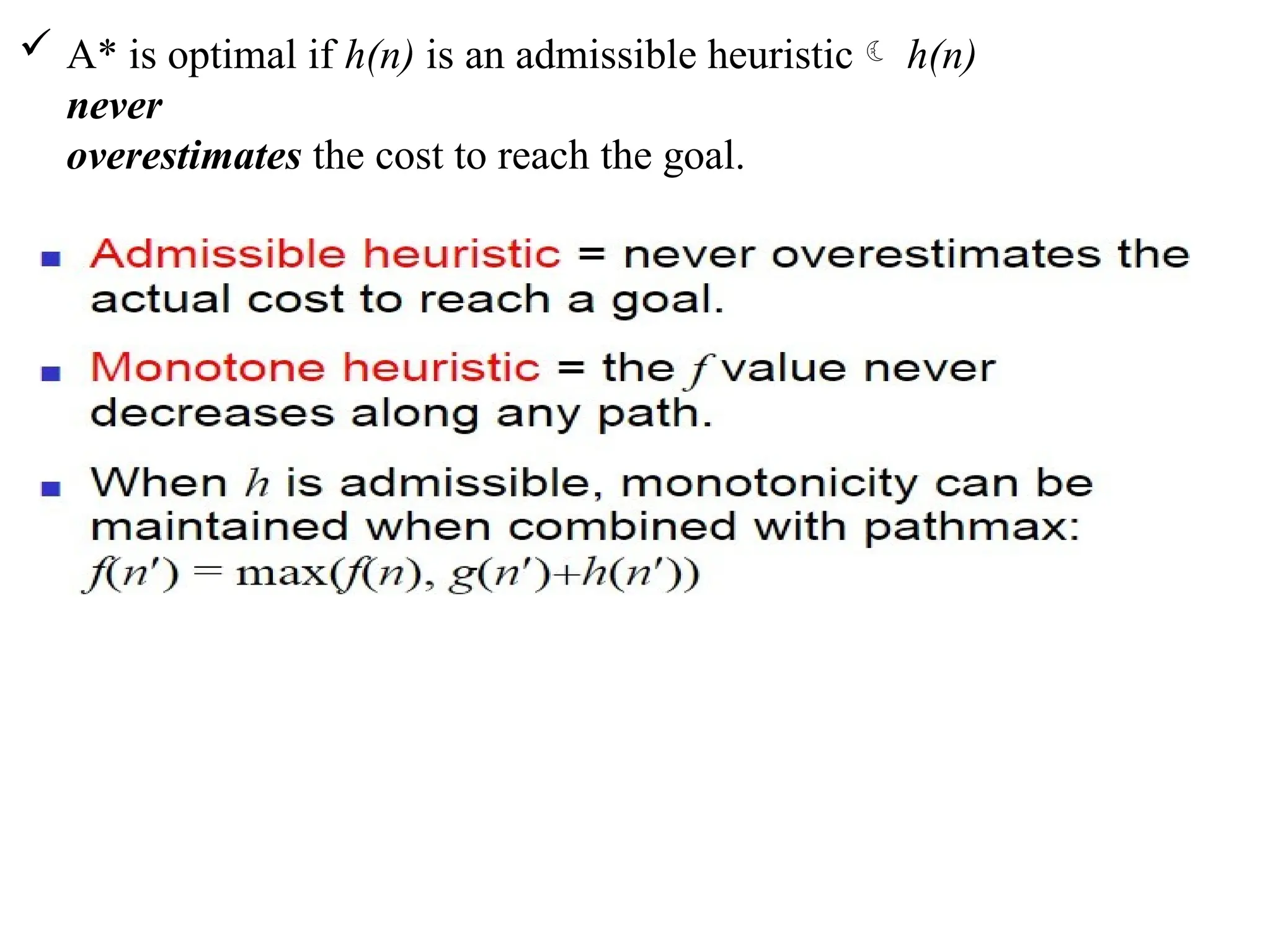
A* isoptimal if h(n) is an admissible heuristic h(n)
never
overestimates the cost to reach the goal.
78.
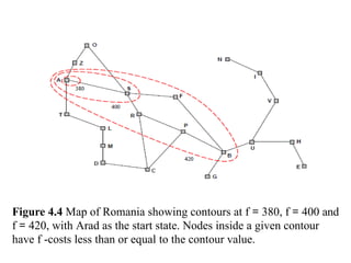
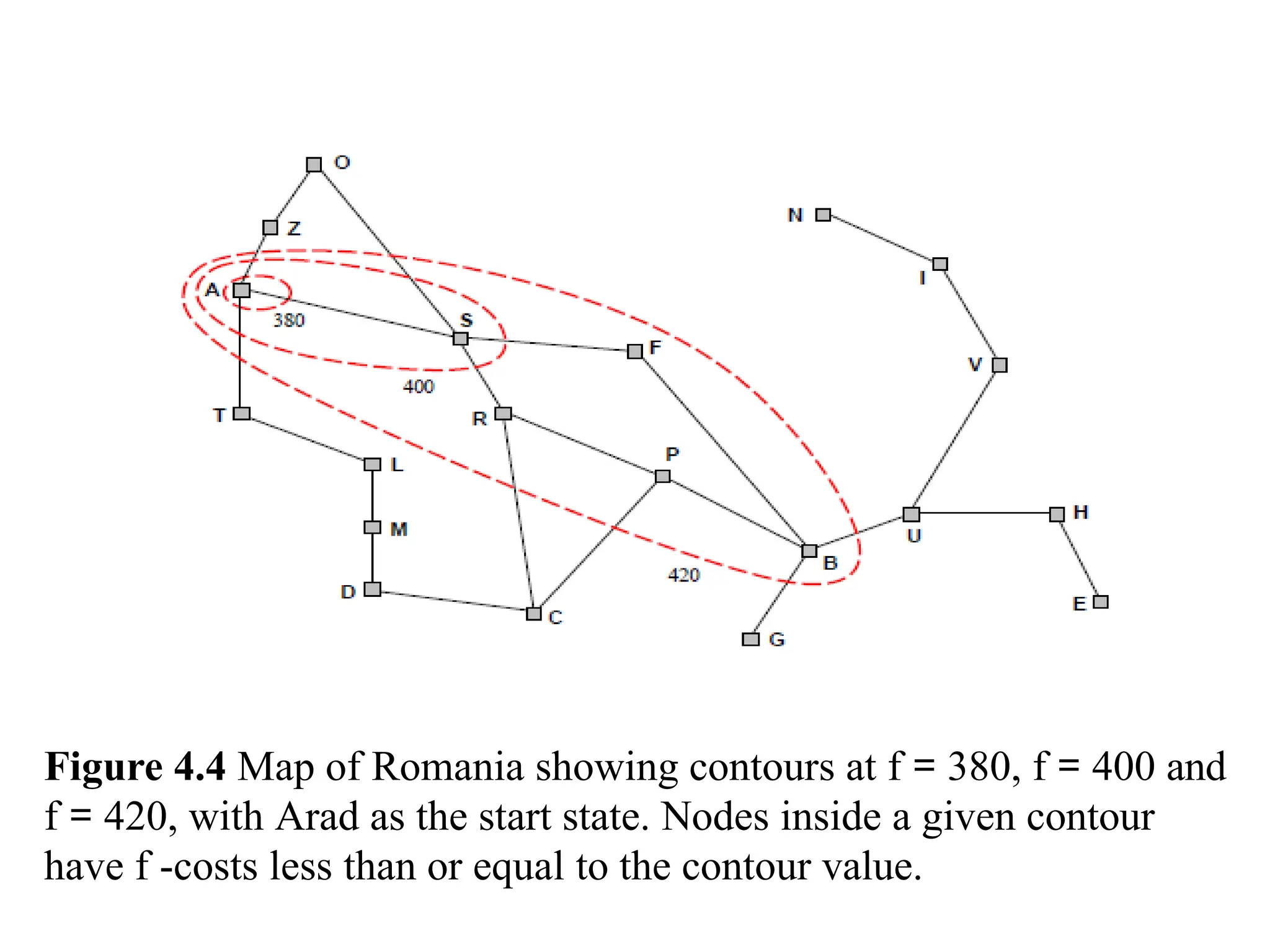
Figure 4.4 Mapof Romania showing contours at f = 380, f = 400 and
f = 420, with Arad as the start state. Nodes inside a given contour
have f -costs less than or equal to the contour value.
79.
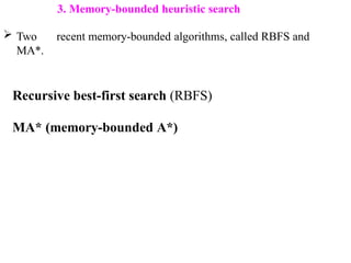
3. Memory-bounded heuristicsearch
Two recent memory-bounded algorithms, called RBFS and
MA*.
Recursive best-first search (RBFS)
MA* (memory-bounded A*)
80.
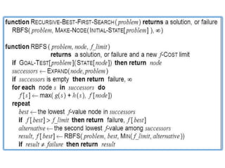
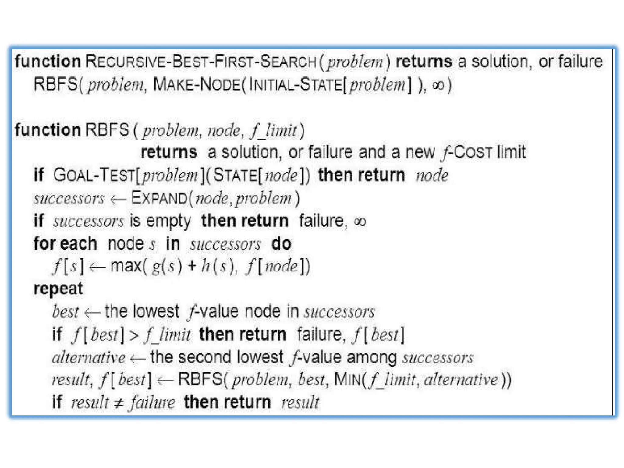
Recursive best-first search(RBFS)
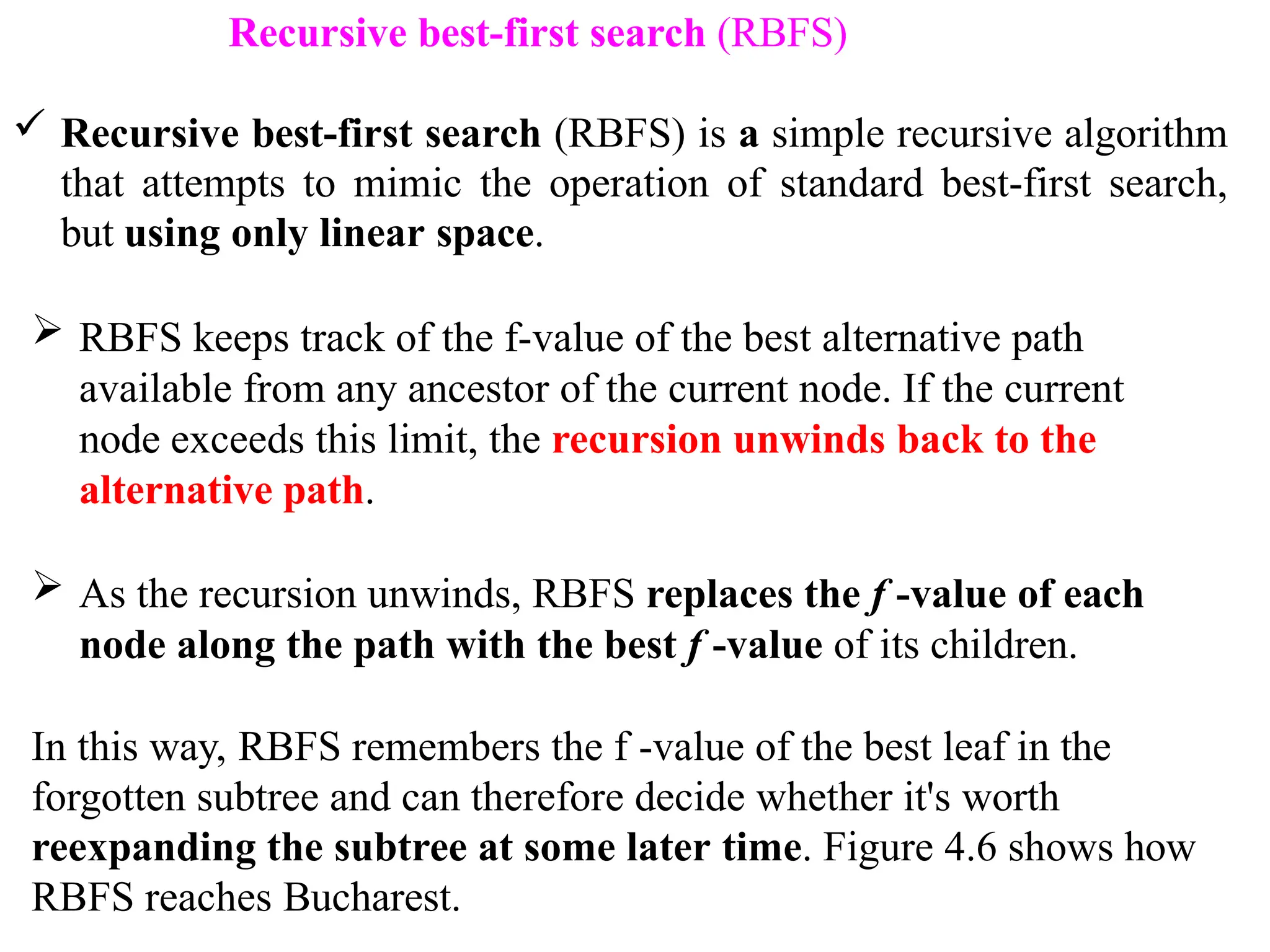
Recursive best-first search (RBFS) is a simple recursive algorithm
that attempts to mimic the operation of standard best-first search,
but using only linear space.
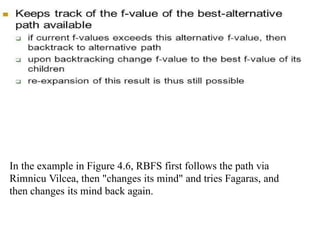
RBFS keeps track of the f-value of the best alternative path
available from any ancestor of the current node. If the current
node exceeds this limit, the recursion unwinds back to the
alternative path.
As the recursion unwinds, RBFS replaces the f -value of each
node along the path with the best f -value of its children.
In this way, RBFS remembers the f -value of the best leaf in the
forgotten subtree and can therefore decide whether it's worth
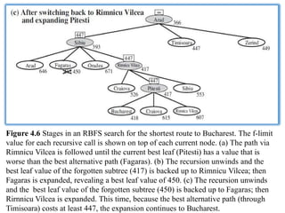
reexpanding the subtree at some later time. Figure 4.6 shows how
RBFS reaches Bucharest.
81.
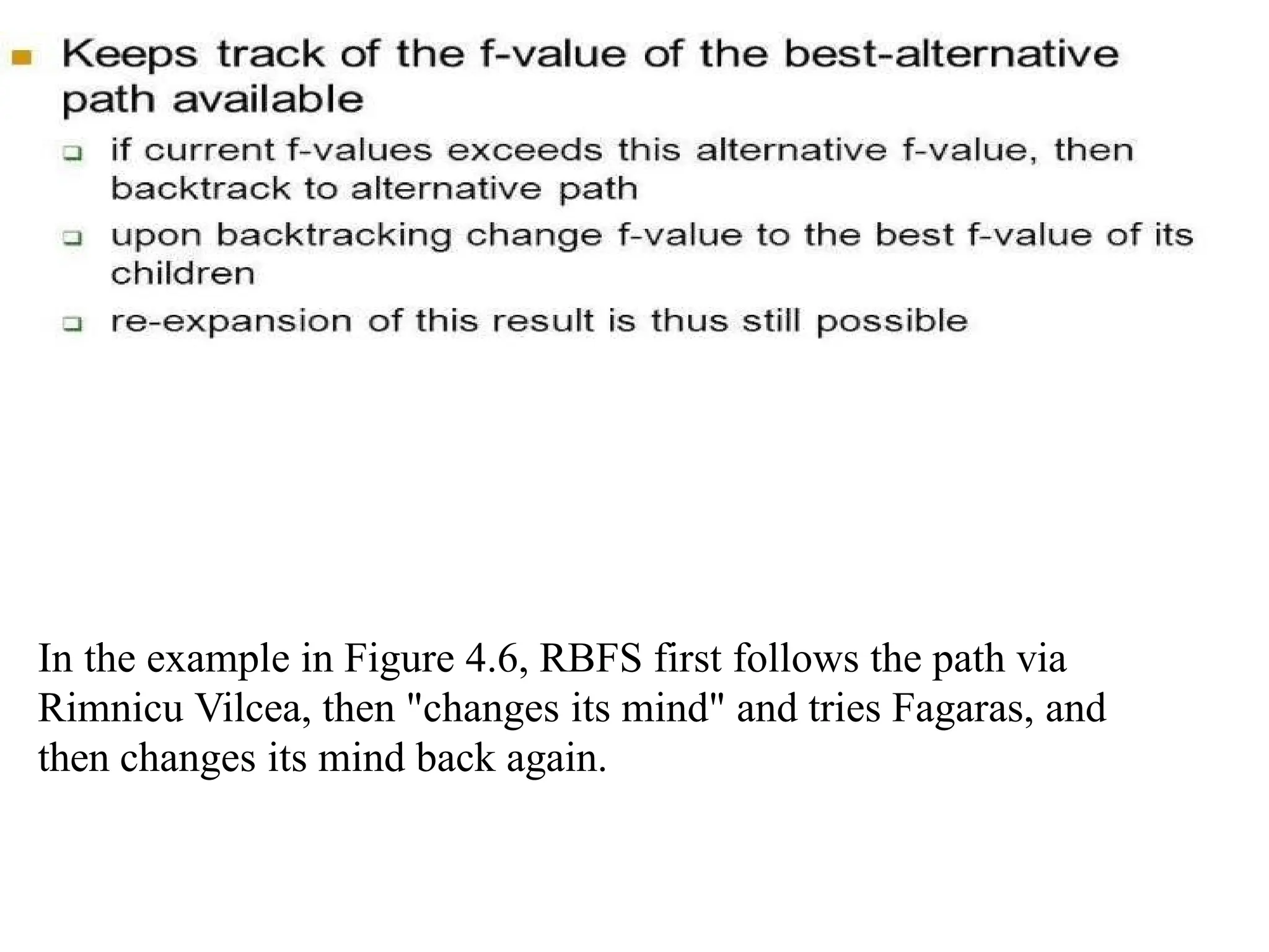
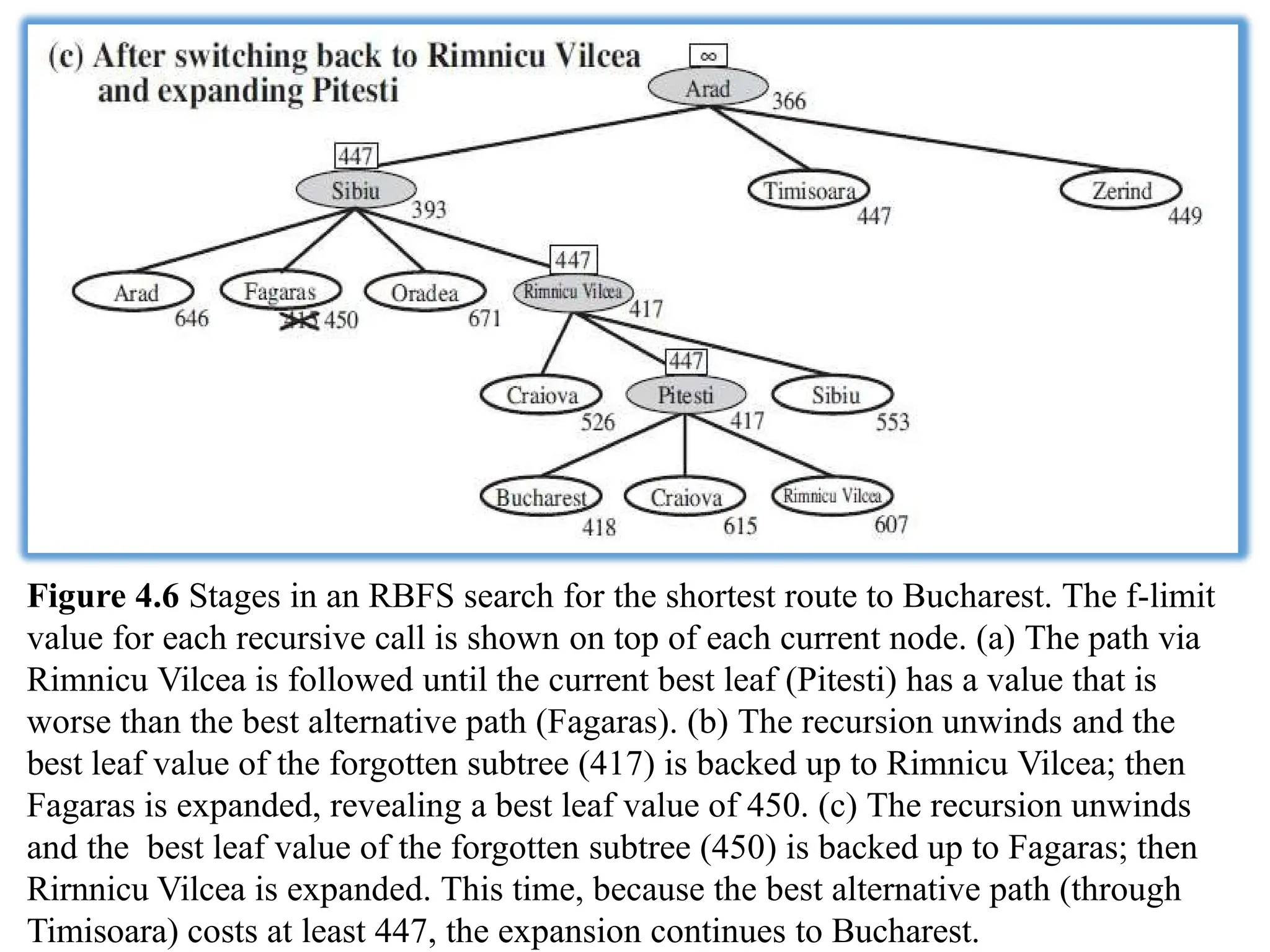
In the examplein Figure 4.6, RBFS first follows the path via
Rimnicu Vilcea, then "changes its mind" and tries Fagaras, and
then changes its mind back again.
84.
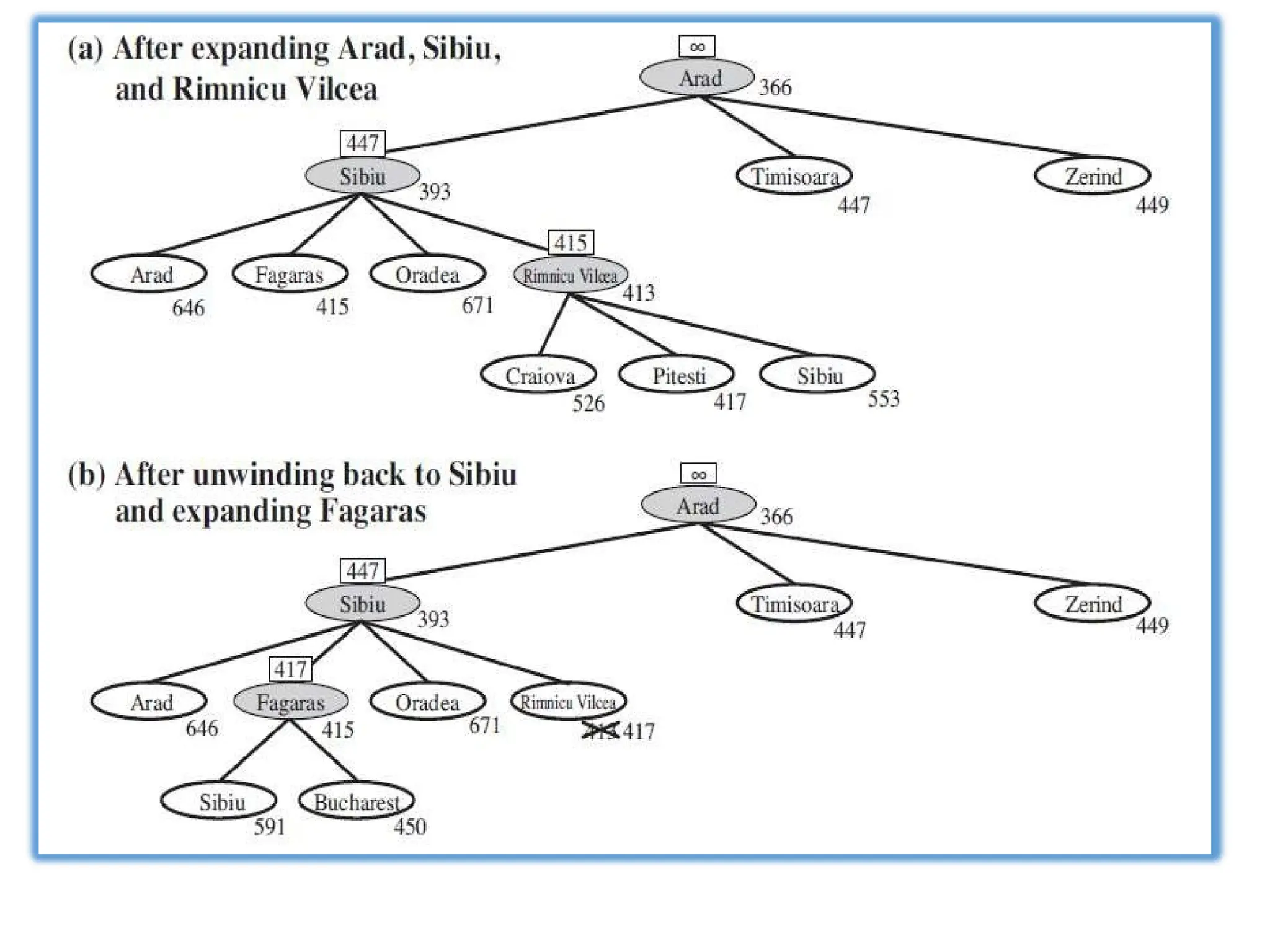
Figure 4.6 Stagesin an RBFS search for the shortest route to Bucharest. The f-limit
value for each recursive call is shown on top of each current node. (a) The path via
Rimnicu Vilcea is followed until the current best leaf (Pitesti) has a value that is
worse than the best alternative path (Fagaras). (b) The recursion unwinds and the
best leaf value of the forgotten subtree (417) is backed up to Rimnicu Vilcea; then
Fagaras is expanded, revealing a best leaf value of 450. (c) The recursion unwinds
and the best leaf value of the forgotten subtree (450) is backed up to Fagaras; then
Rirnnicu Vilcea is expanded. This time, because the best alternative path (through
Timisoara) costs at least 447, the expansion continues to Bucharest.
85.
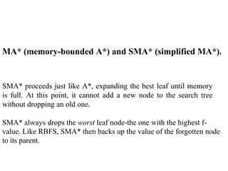
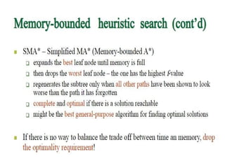
MA* (memory-bounded A*)and SMA* (simplified MA*).
SMA* proceeds just like A*, expanding the best leaf until memory
is full. At this point, it cannot add a new node to the search tree
without dropping an old one.
SMA* always drops the worst leaf node-the one with the highest f-
value. Like RBFS, SMA* then backs up the value of the forgotten node
to its parent.
87.
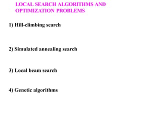
LOCAL SEARCH ALGORITHMSAND
OPTIMIZATION PROBLEMS
Local search algorithms operate using a single current state (rather
than multiple paths) and generally move only to neighbours of that
state.
Typically, the paths followed by the search are not retained. Although
local search algorithms are not systematic, they have two key
advantages:
(1) they use very little memory-usually a constant amount; and
(2) they can often find reasonable solutions in large or infinite
(continuous) state spaces for which systematic algorithms are
unsuitable.
89.
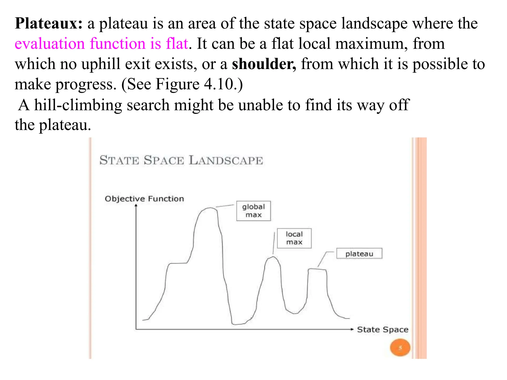
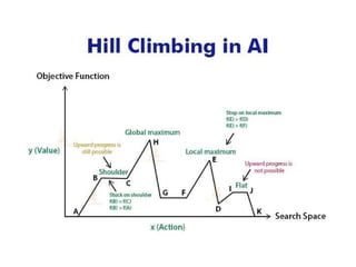
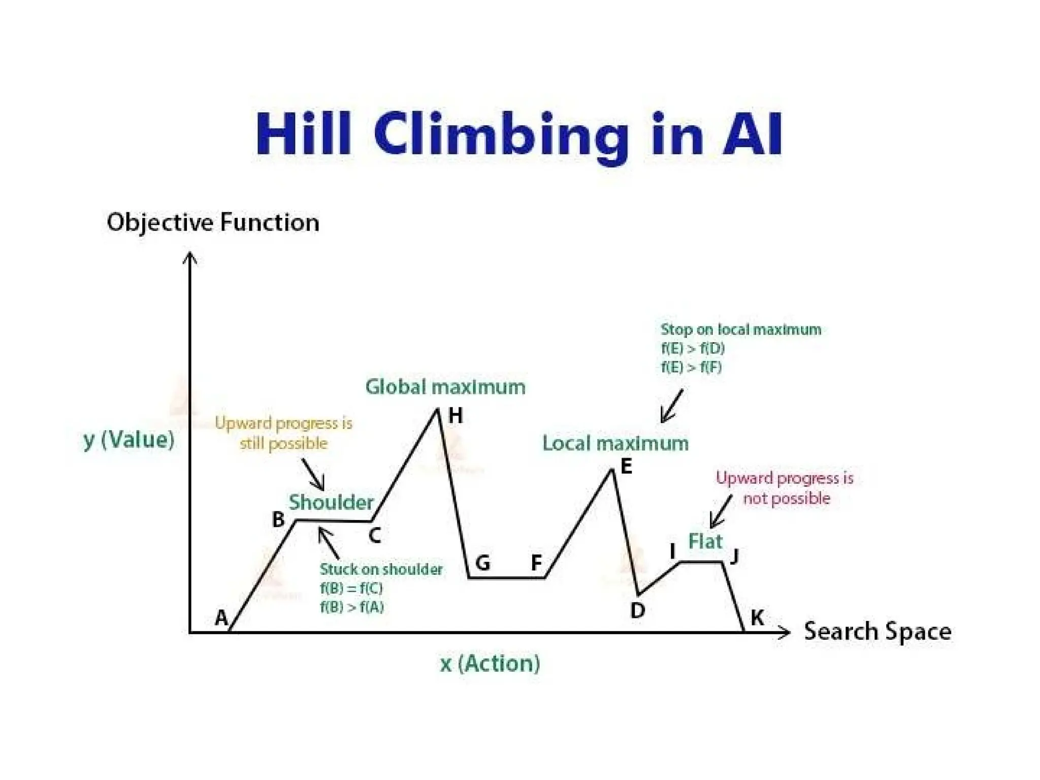
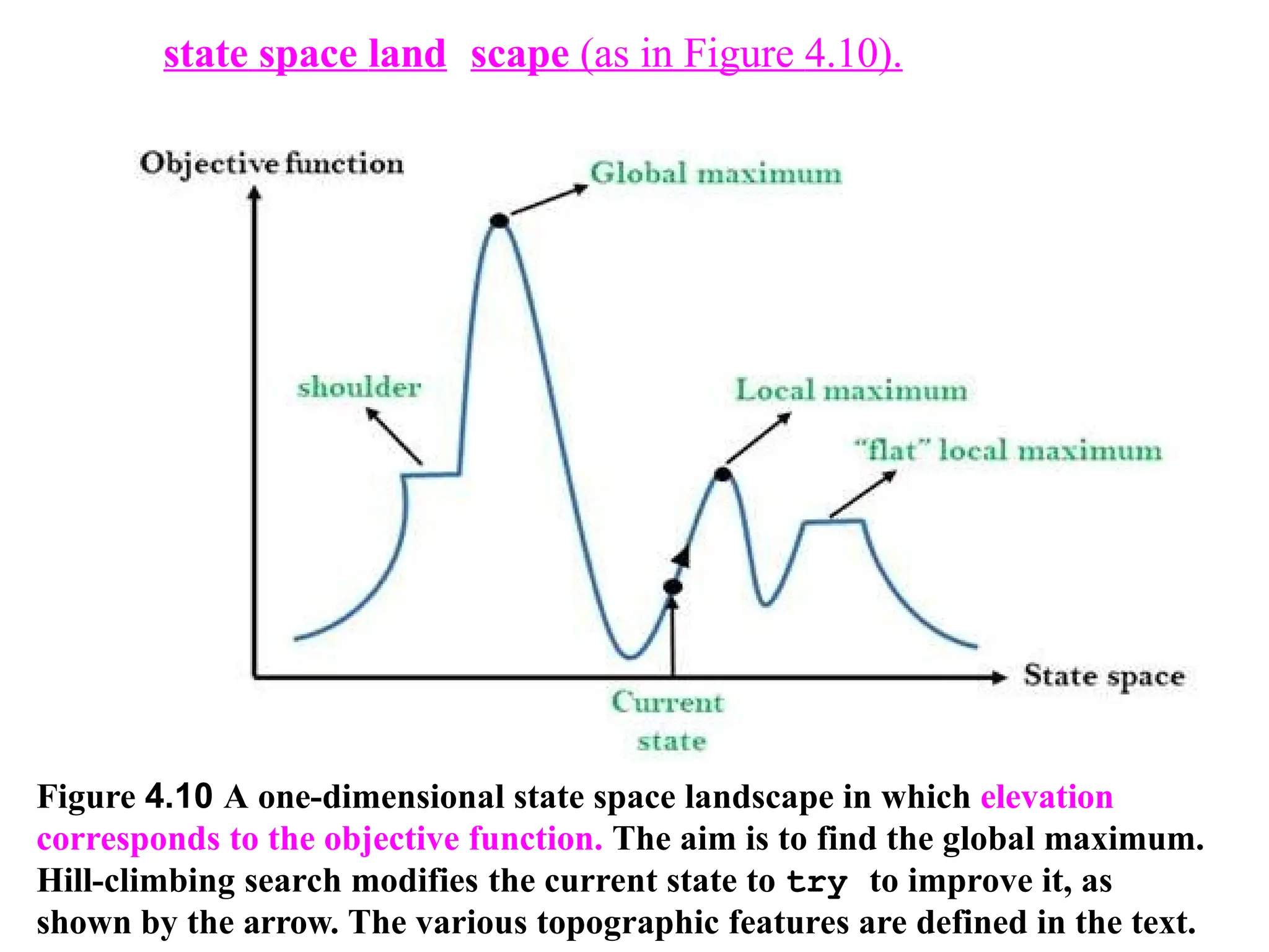
Figure 4.10 Aone-dimensional state space landscape in which elevation
corresponds to the objective function. The aim is to find the global maximum.
Hill-climbing search modifies the current state to try to improve it, as
shown by the arrow. The various topographic features are defined in the text.
state space land scape (as in Figure 4.10).
90.
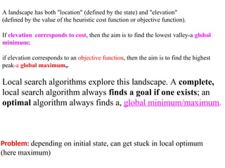
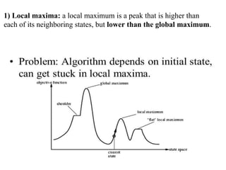
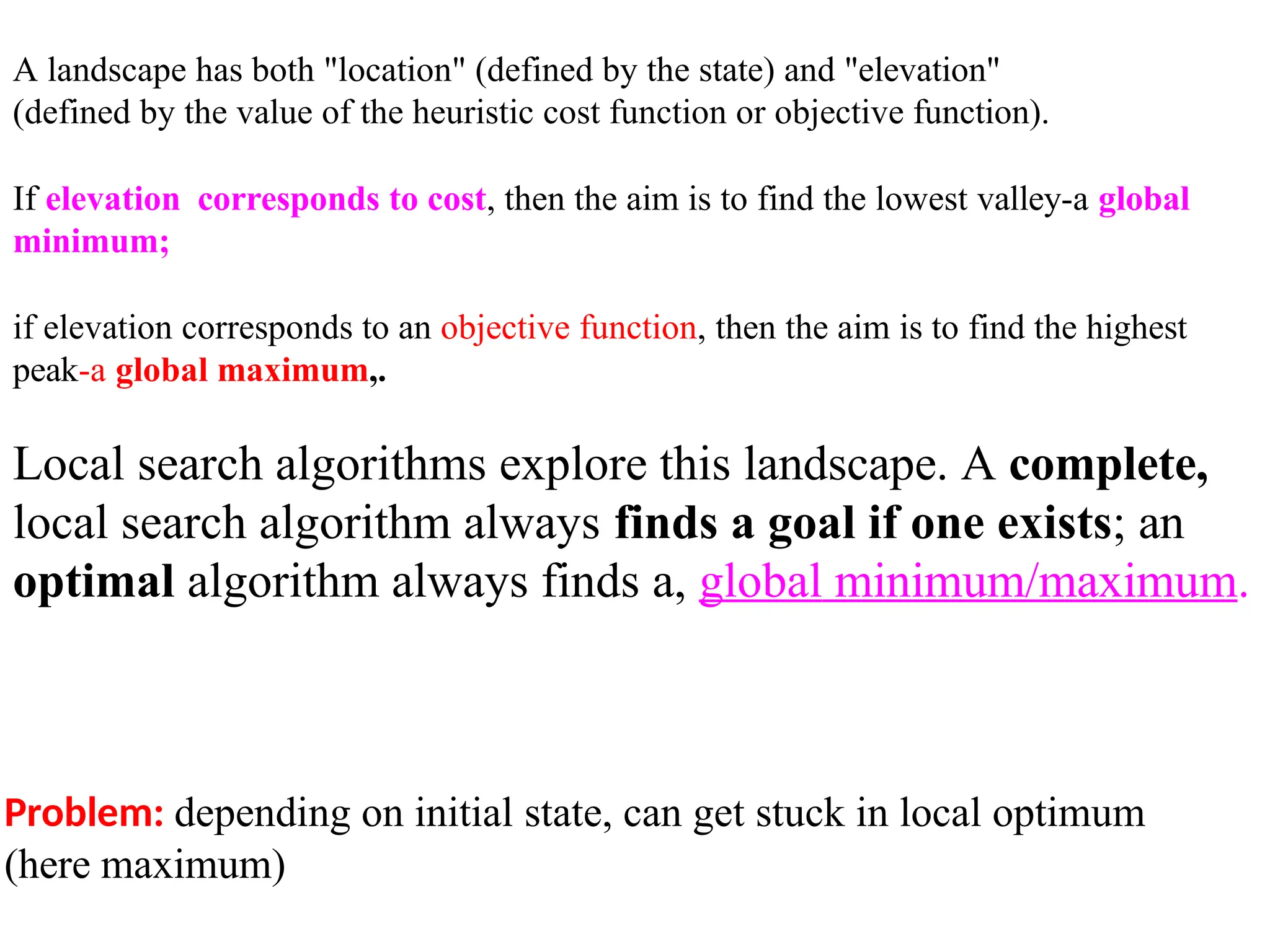
Problem: depending oninitial state, can get stuck in local optimum
(here maximum)
A landscape has both "location" (defined by the state) and "elevation"
(defined by the value of the heuristic cost function or objective function).
If elevation corresponds to cost, then the aim is to find the lowest valley-a global
minimum;
if elevation corresponds to an objective function, then the aim is to find the highest
peak-a global maximum,.
Local search algorithms explore this landscape. A complete,
local search algorithm always finds a goal if one exists; an
optimal algorithm always finds a, global minimum/maximum.
91.
1) Hill-climbing search
2)Simulated annealing search
3) Local beam search
4) Genetic algorithms
LOCAL SEARCH ALGORITHMS AND
OPTIMIZATION PROBLEMS
93.
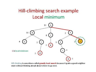
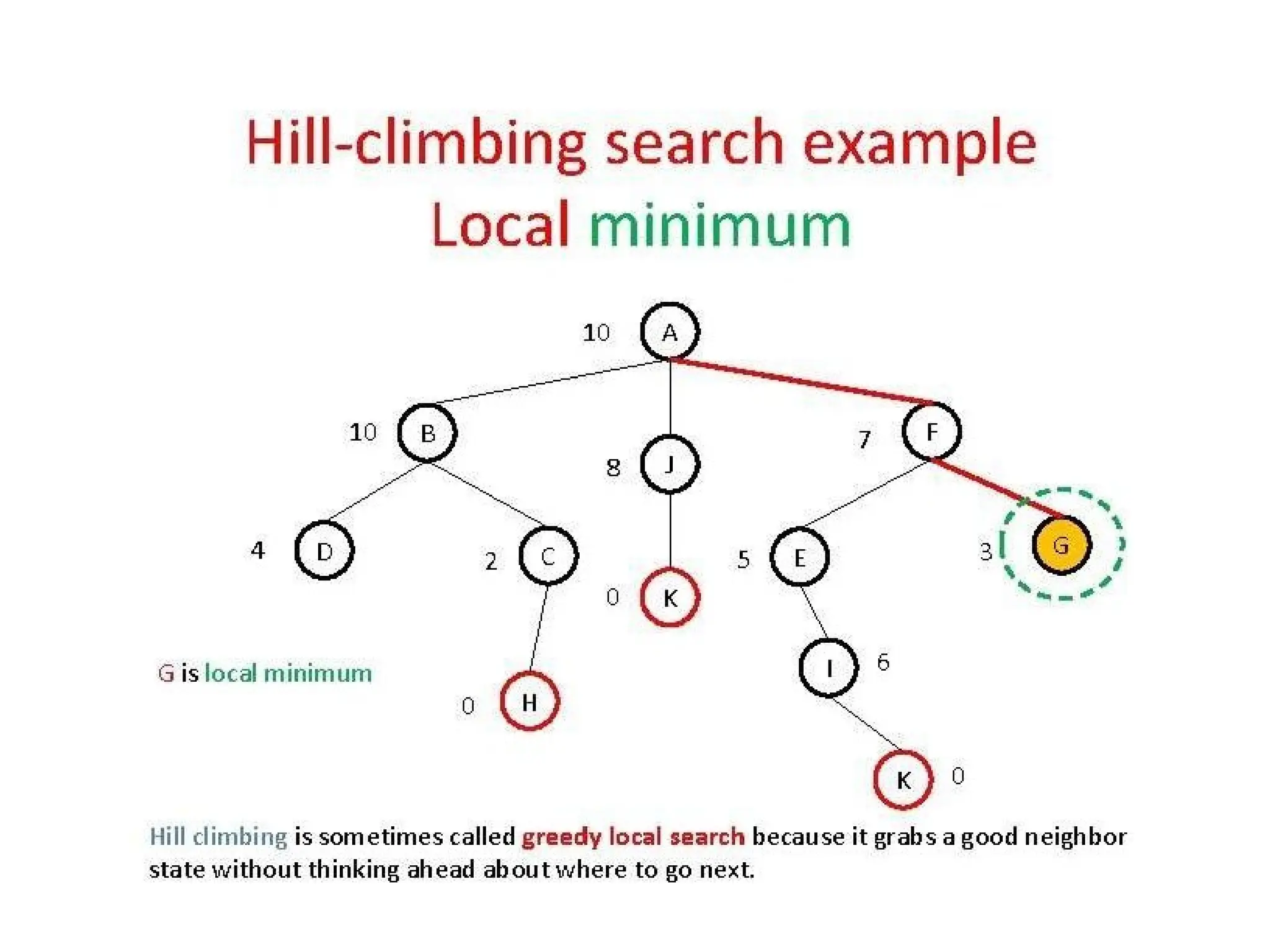
HILL-CLIMBING SEARCH
(cont.)
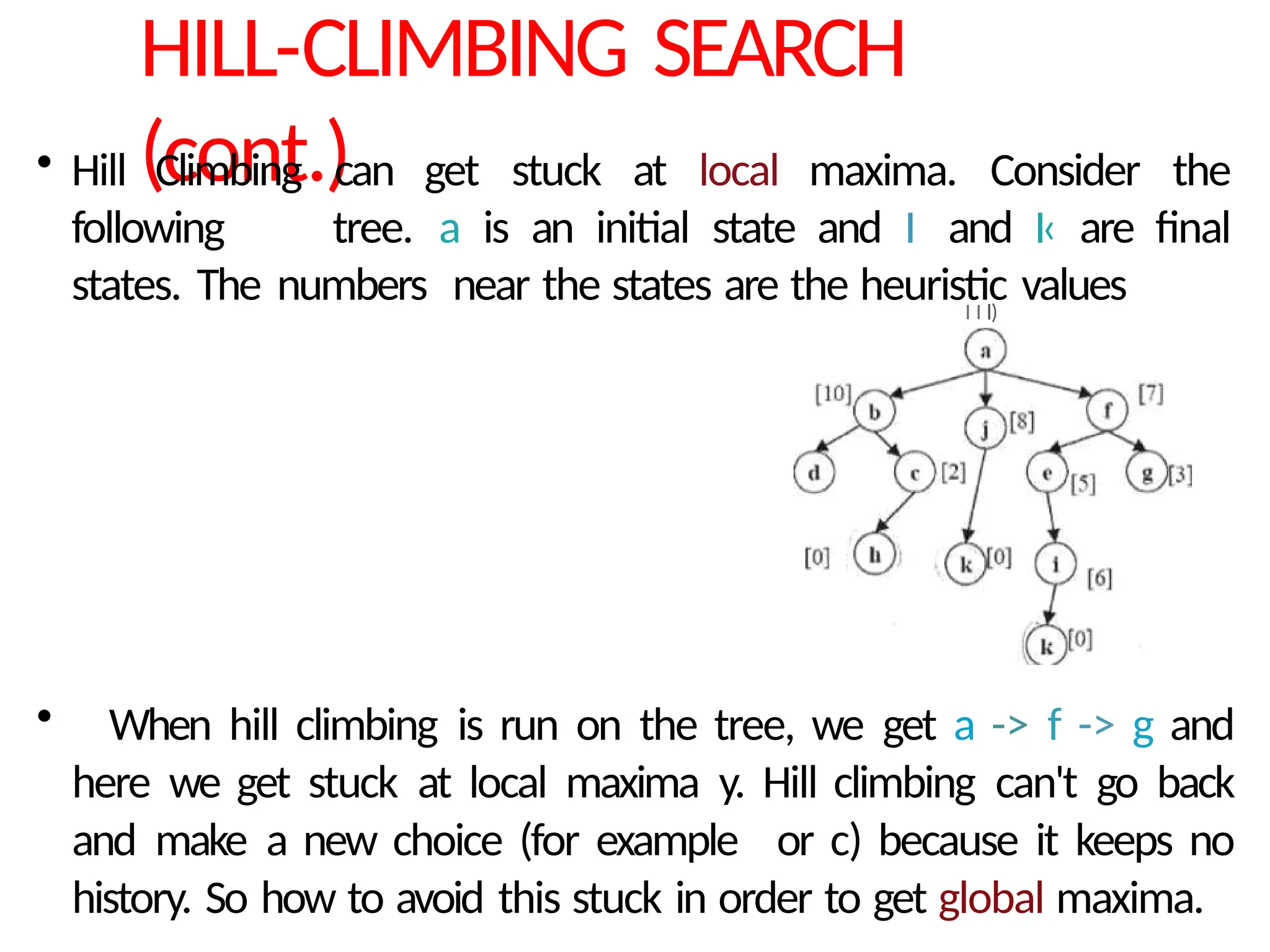
• HillClimbing can get stuck at local maxima. Consider the
following tree. a is an initial state and I and I‹ are final
states. The numbers near the states are the heuristic values
I I l)
• When hill climbing is run on the tree, we get a -> f -> g and
here we get stuck at local maxima y. Hill climbing can't go back
and make a new choice (for example or c) because it keeps no
history. So how to avoid this stuck in order to get global maxima.
94.
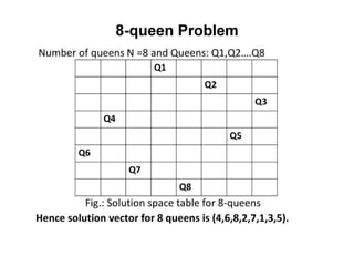
1) Hill-climbing search
It is simply a loop that continually moves in the direction of
increasing value-that is, uphill. It terminates when it reaches a
"peak" where no neighbor has a higher value.
function HILL-CLIMBING(problem) returns a state that is a local
maximum
inputs: problem, a problem
local variables: current, a node
neighbour, a node
current MAKENODE(INITIAL-STATE [problem])
loop do
neighbour a highest-valued successor of current
if Value[neighbour] <= Value[current] then return STATE [current ]
current neighbour
Figure 4.11 The hill-climbing search algorithm, which is the most basic local search
technique. At each step the current node is replaced by the best neighbor; in this
version, that means the neighbor with the highest VALUE, but if a heuristic cost
95.
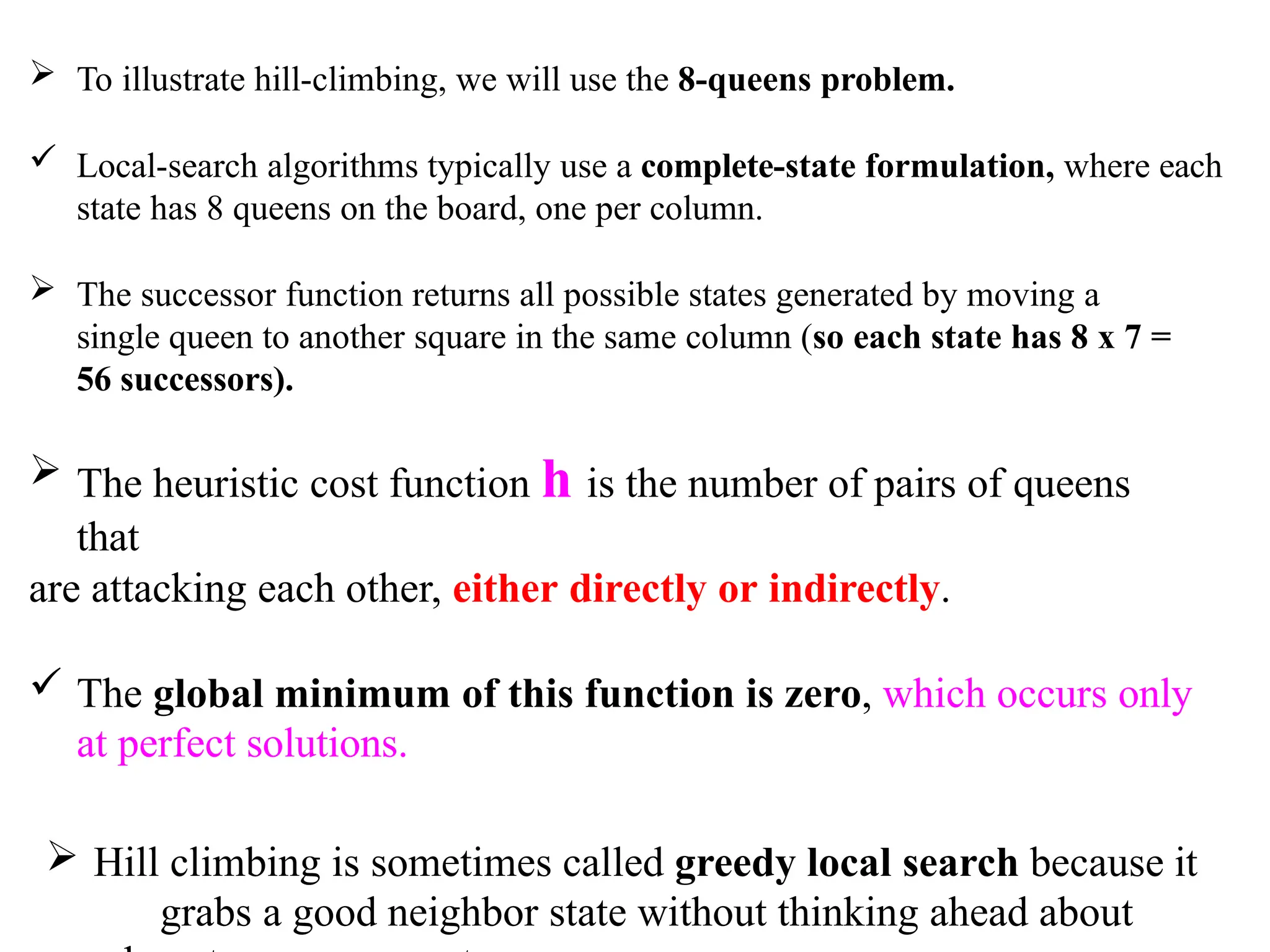
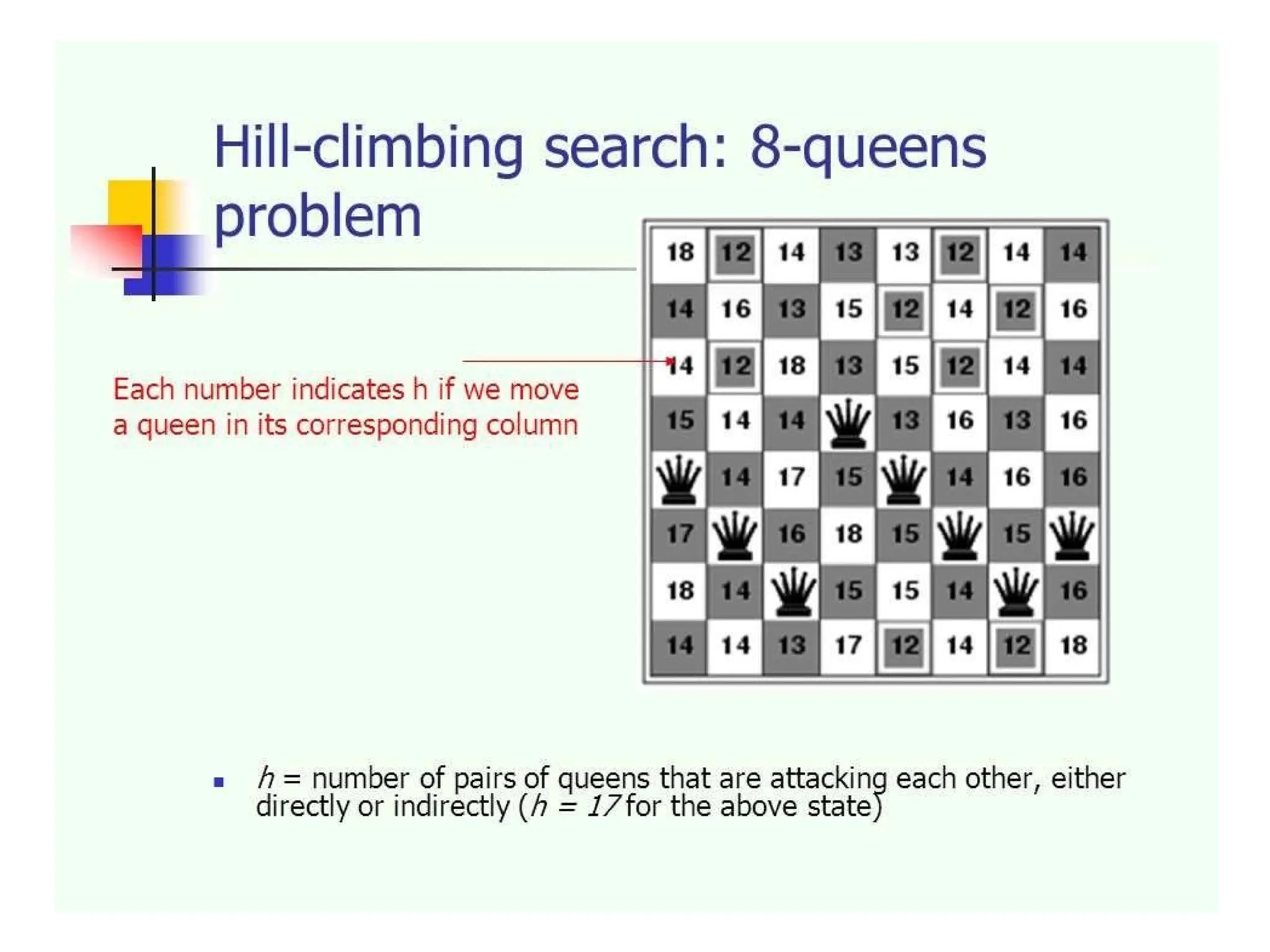
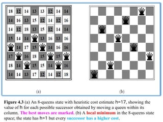
To illustratehill-climbing, we will use the 8-queens problem.
Local-search algorithms typically use a complete-state formulation, where each
state has 8 queens on the board, one per column.
The successor function returns all possible states generated by moving a
single queen to another square in the same column (so each state has 8 x 7 =
56 successors).
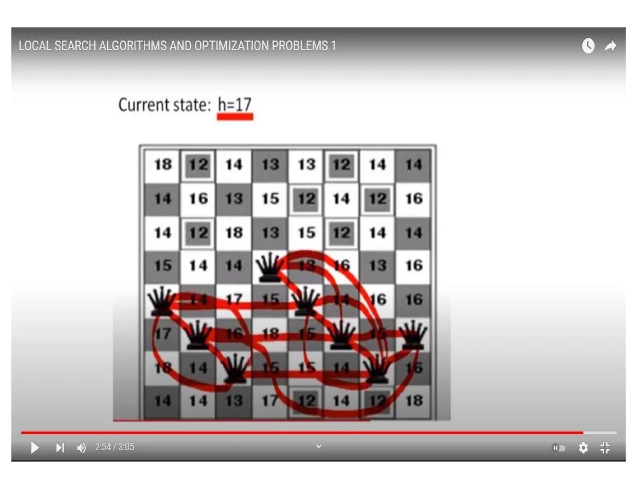
The heuristic cost function h is the number of pairs of queens
that
are attacking each other, either directly or indirectly.
The global minimum of this function is zero, which occurs only
at perfect solutions.
Hill climbing is sometimes called greedy local search because it
grabs a good neighbor state without thinking ahead about
96.
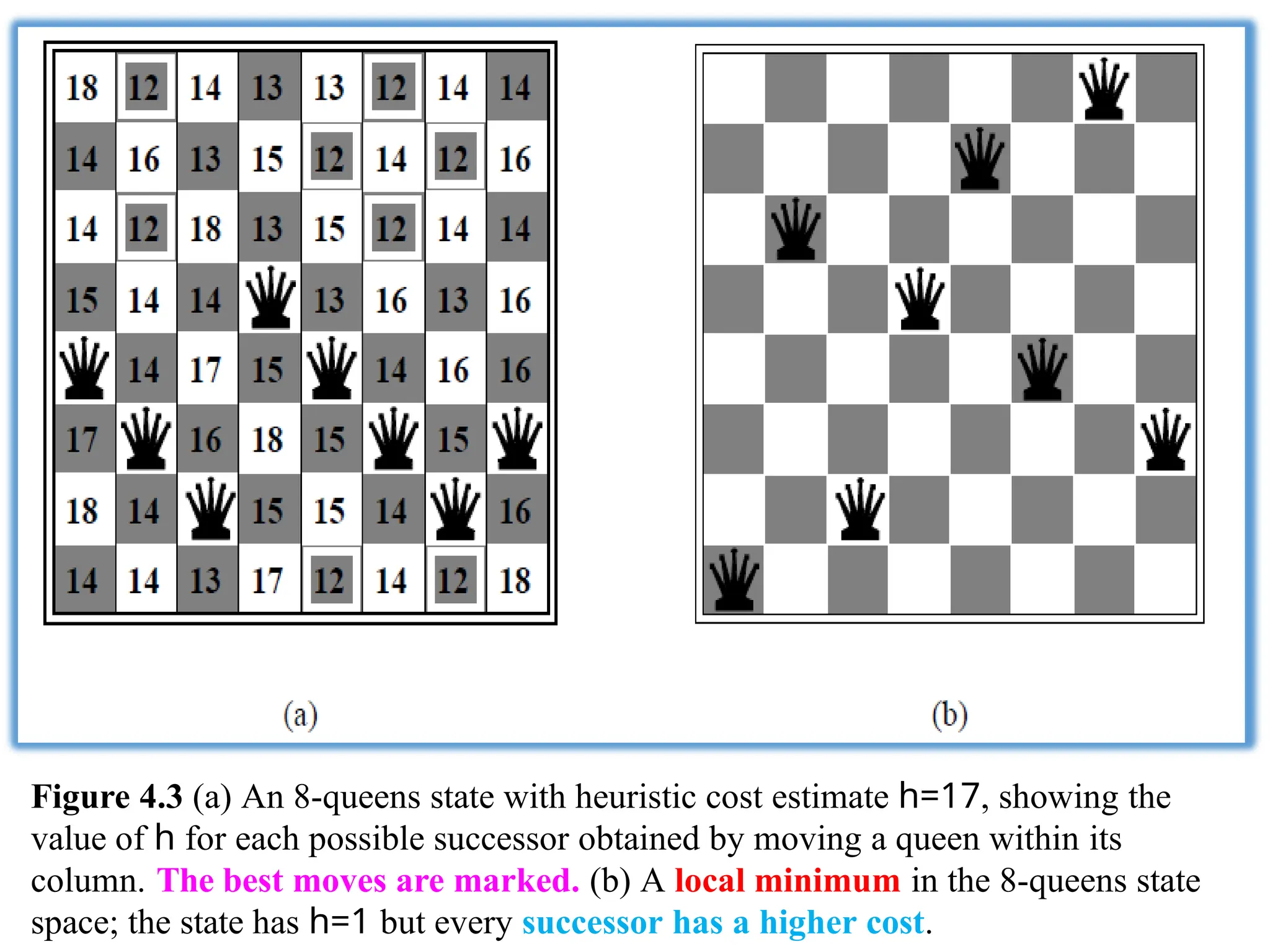
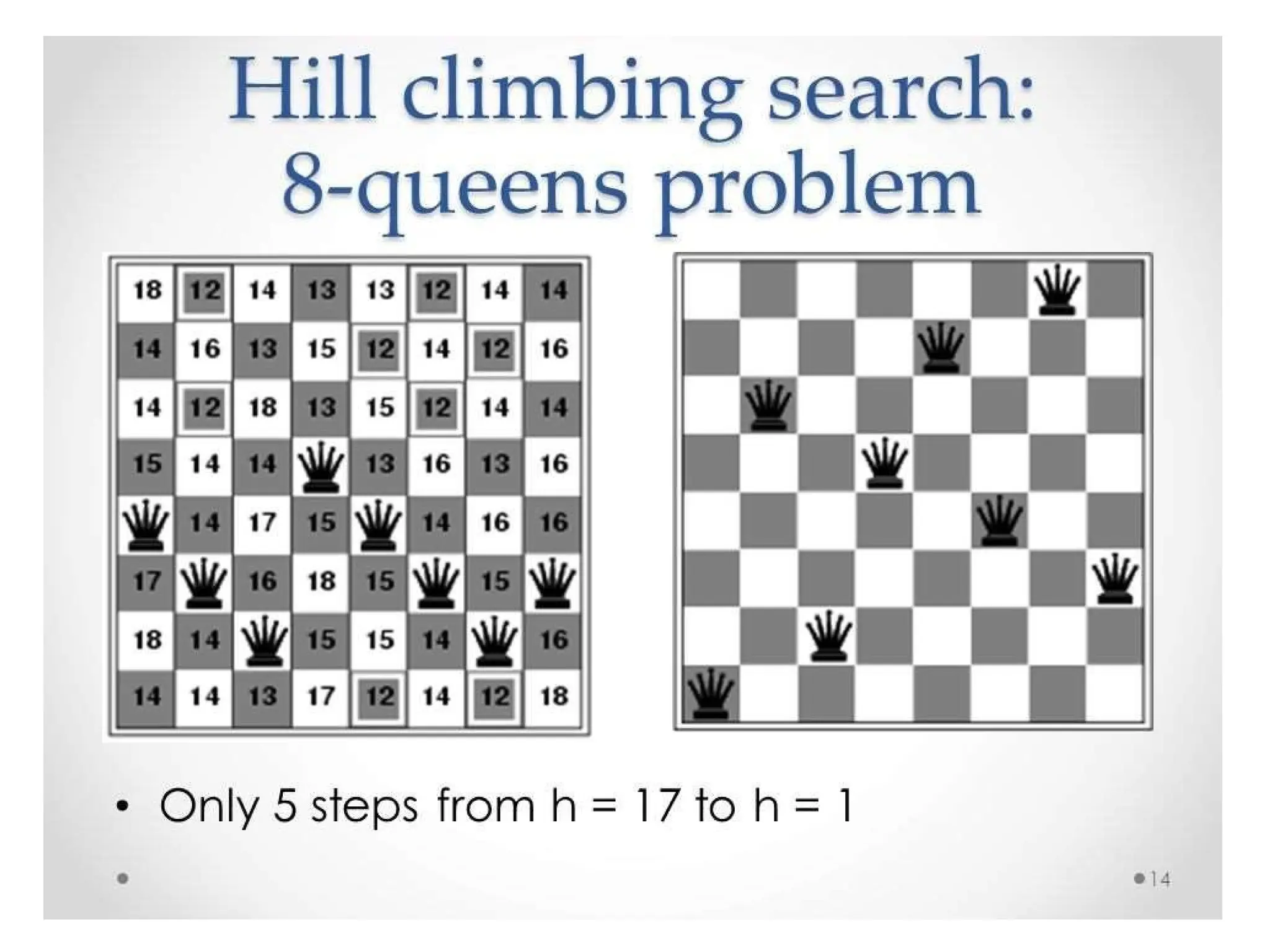
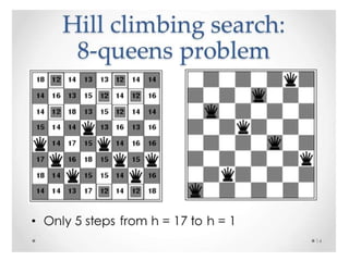
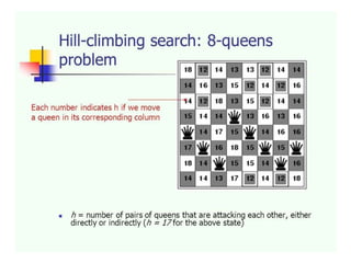
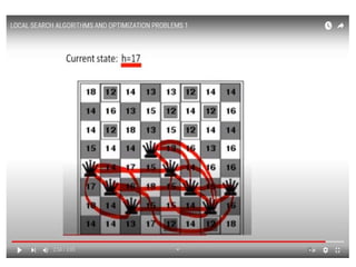
Figure 4.3 (a)An 8-queens state with heuristic cost estimate h=17, showing the
value of h for each possible successor obtained by moving a queen within its
column. The best moves are marked. (b) A local minimum in the 8-queens state
space; the state has h=1 but every successor has a higher cost.
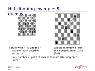
98.
Hill-climbing example: 8-
queens
Astate with fi--17 and the fi-
value for each possible
successor
A local minimum of h in
the 8-queens state space
(fi--1).
h -- number of pairs of queens that are attacking each
other
CIS 391 - Inn o
to .xI
gg'Pen
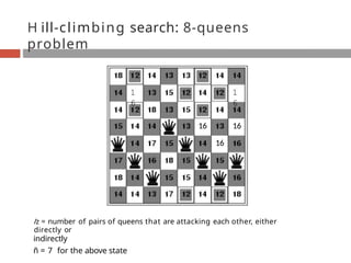
99.
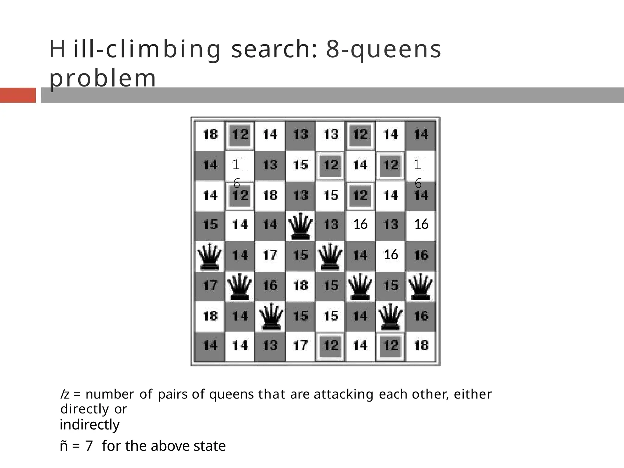
H ill-climbing search:8-queens
problem
1
6
1
6
16 16
16
/z = number of pairs of queens that are attacking each other, either
directly or
indirectly
ñ = 7 for the above state
100.
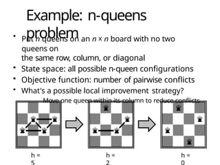
Example: n-queens
problem
• Putn queens on an n x n board with no two
queens on
the same row, column, or diagonal
• State space: all possible n-queen configurations
• Objective function: number of pairwise conflicts
• What's a possible local improvement strategy?
— Move one queen within its column to reduce conflicts
h = h = h =
103.
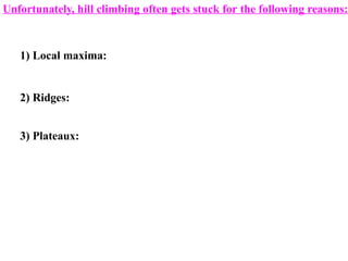
1) Local maxima:
2)Ridges:
3) Plateaux:
Unfortunately, hill climbing often gets stuck for the following reasons:
104.
1) Local maxima:a local maximum is a peak that is higher than
each of its neighboring states, but lower than the global maximum.
105.
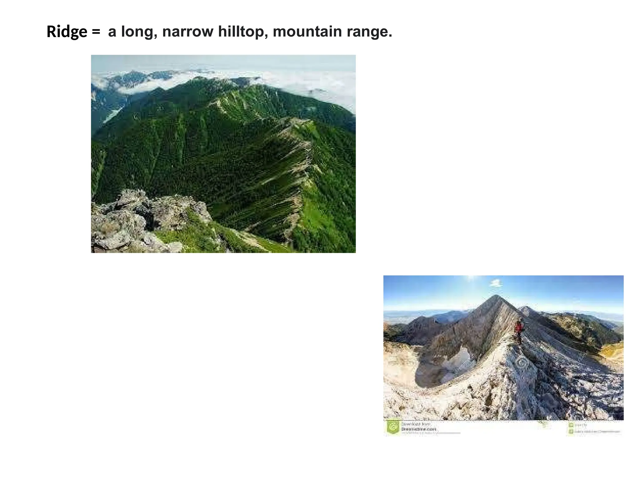
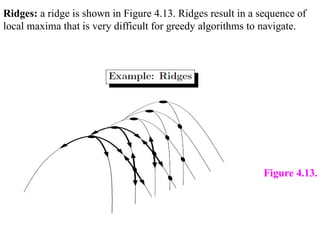
Ridges: a ridgeis shown in Figure 4.13. Ridges result in a sequence of
local maxima that is very difficult for greedy algorithms to navigate.
Figure 4.13.
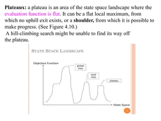
Plateaux: a plateauis an area of the state space landscape where the
evaluation function is flat. It can be a flat local maximum, from
which no uphill exit exists, or a shoulder, from which it is possible to
make progress. (See Figure 4.10.)
A hill-climbing search might be unable to find its way off
the plateau.
108.
A plateau isa flat, elevated landform that rises sharply above the
surrounding
area on at least one side
111.
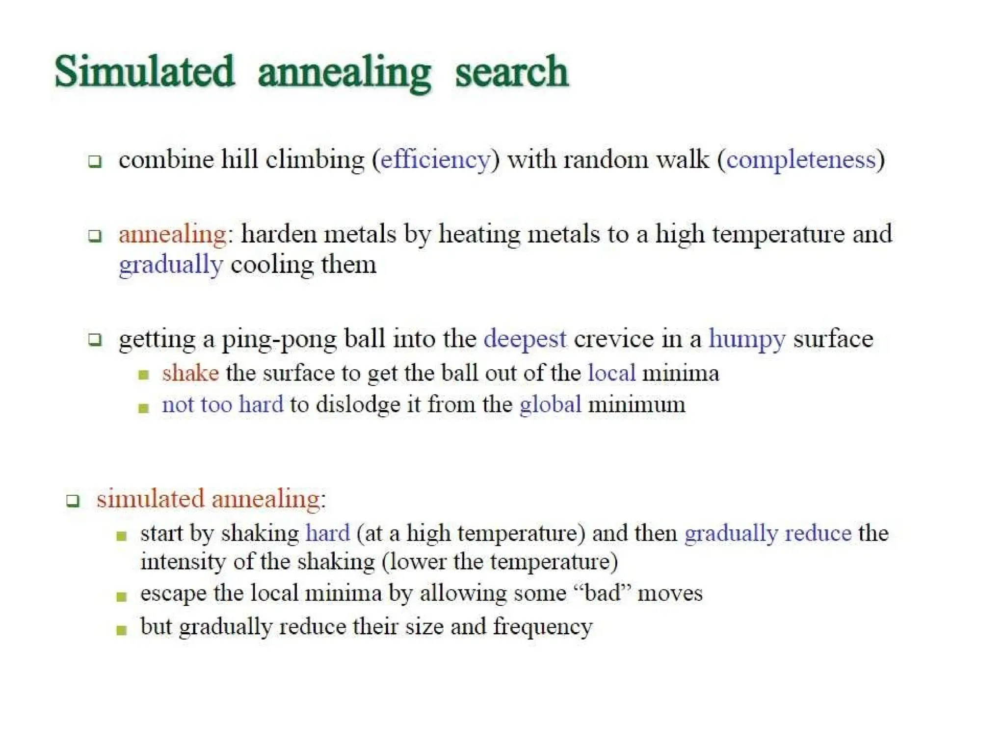
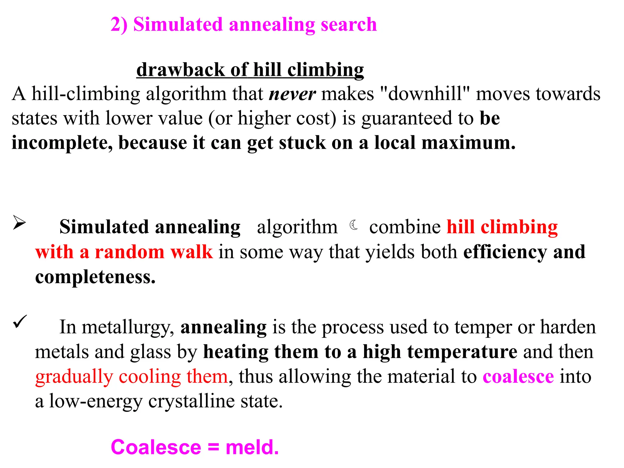
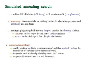
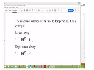
2) Simulated annealingsearch
drawback of hill climbing
A hill-climbing algorithm that never makes "downhill" moves towards
states with lower value (or higher cost) is guaranteed to be
incomplete, because it can get stuck on a local maximum.
Simulated annealing algorithm combine hill climbing
with a random walk in some way that yields both efficiency and
completeness.
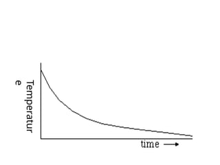
In metallurgy, annealing is the process used to temper or harden
metals and glass by heating them to a high temperature and then
gradually cooling them, thus allowing the material to coalesce into
a low-energy crystalline state.
Coalesce = meld.
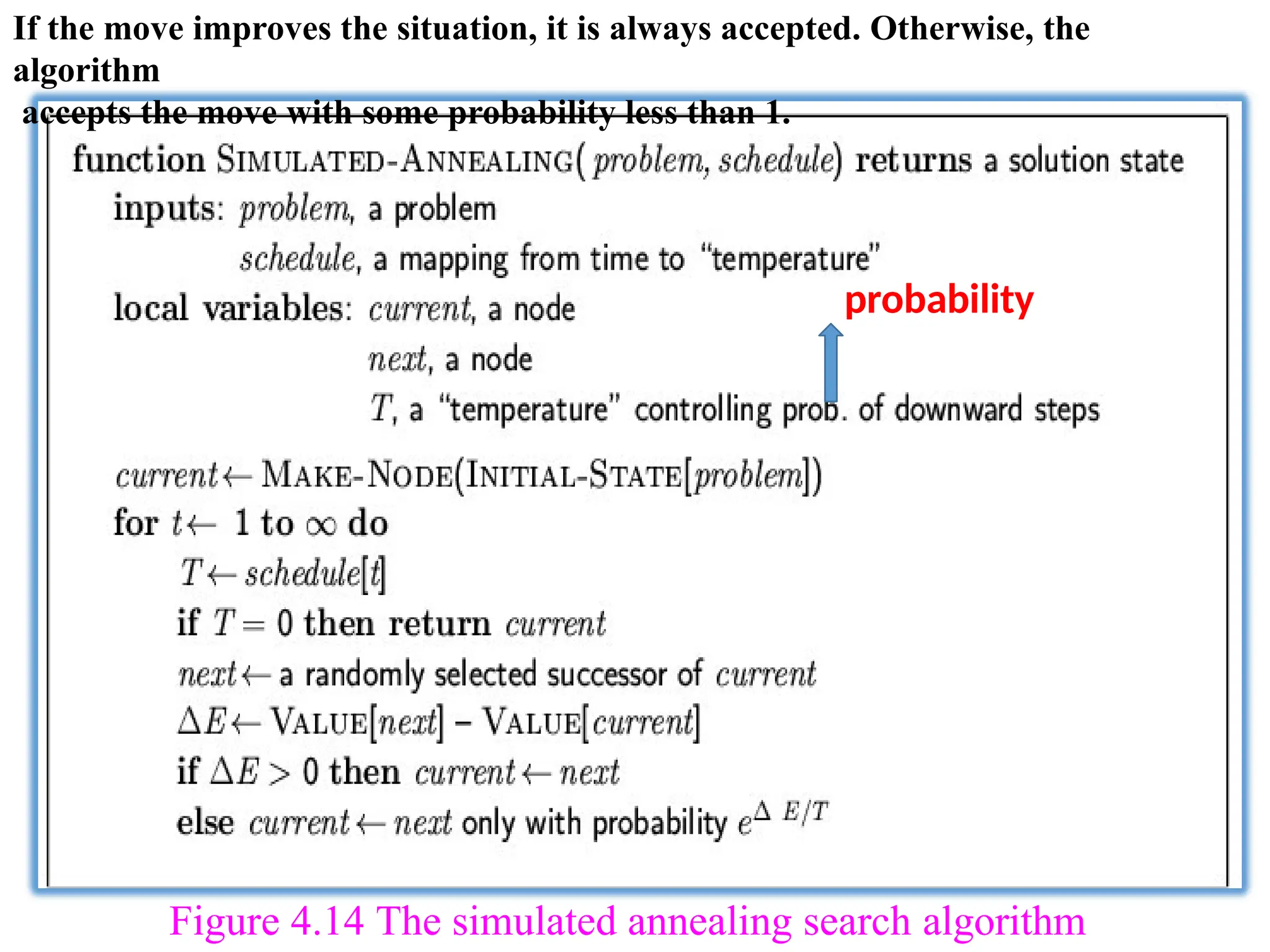
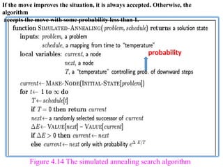
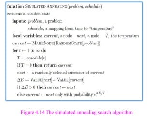
112.
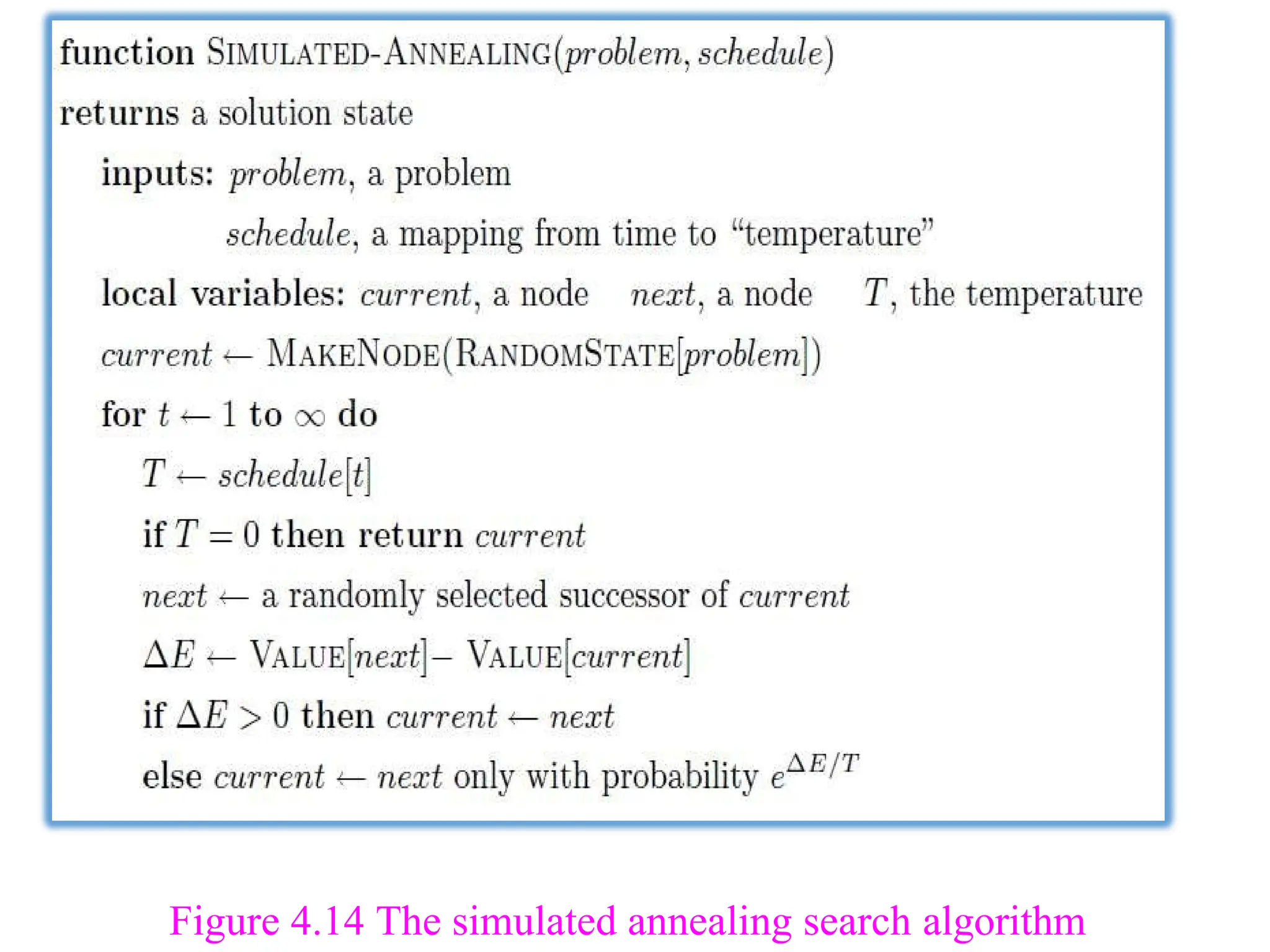
Figure 4.14 Thesimulated annealing search algorithm
If the move improves the situation, it is always accepted. Otherwise, the
algorithm
accepts the move with some probability less than 1.
probability
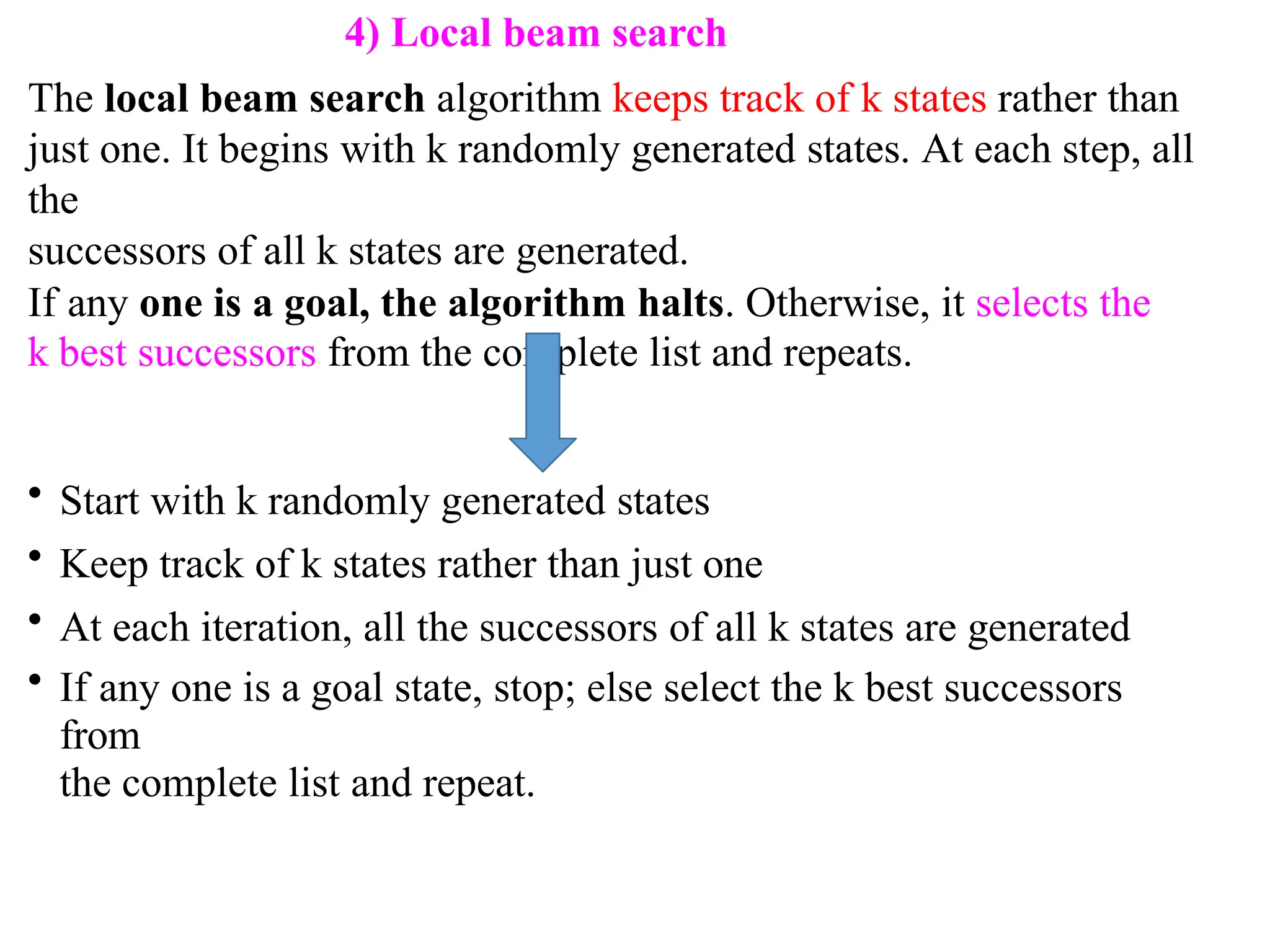
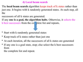
4) Local beamsearch
The local beam search algorithm keeps track of k states rather than
just one. It begins with k randomly generated states. At each step, all
the
successors of all k states are generated.
If any one is a goal, the algorithm halts. Otherwise, it selects the
k best successors from the complete list and repeats.
• Start with k randomly generated states
• Keep track of k states rather than just one
• At each iteration, all the successors of all k states are generated
• If any one is a goal state, stop; else select the k best successors
from
the complete list and repeat.
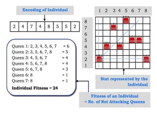
Genetic algorithms
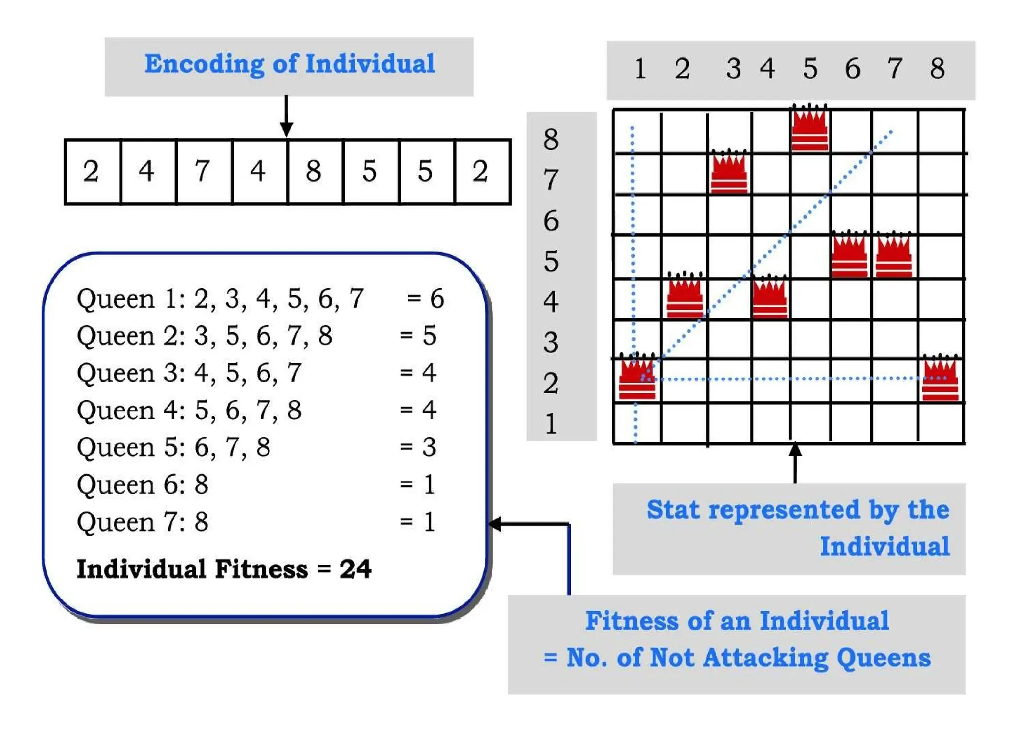
Likebeam search, GAS begin with a set of k randomly generated
states, called the population. Each state, or individual, is
represented as a string over a finite alphabet most commonly, a
string of 0s and 1s.
For example, an 8-queens state must specify the positions of
8 queens, each in a column of 8 squares.
Figure 4.15(a) shows a population of four 8-digit strings representing
8-queens states.
121.
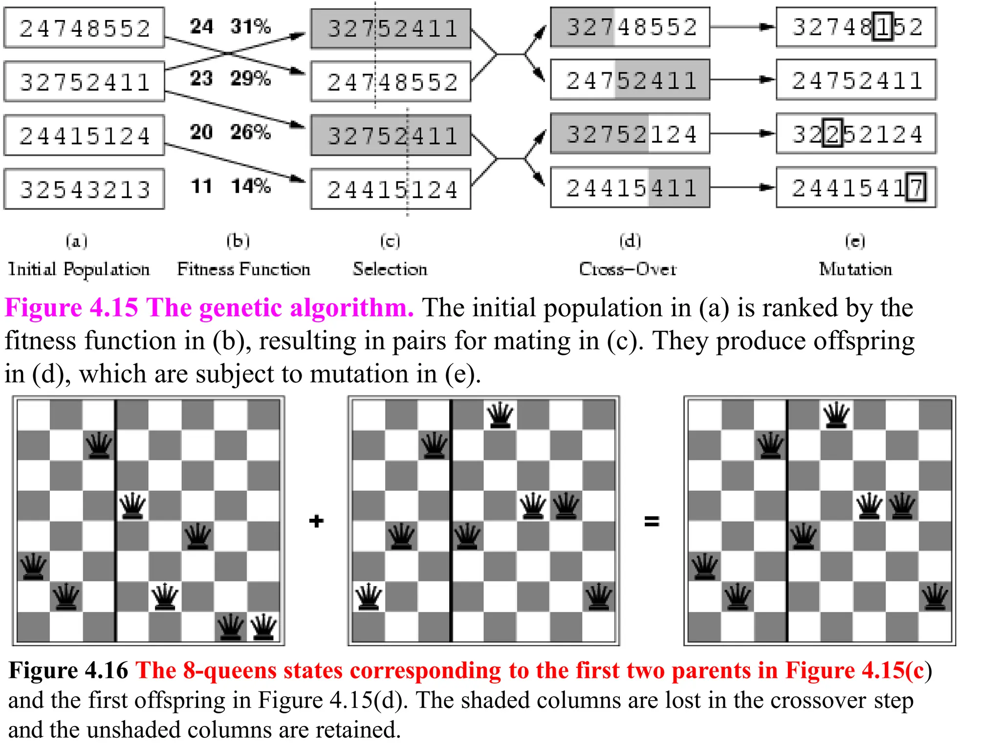
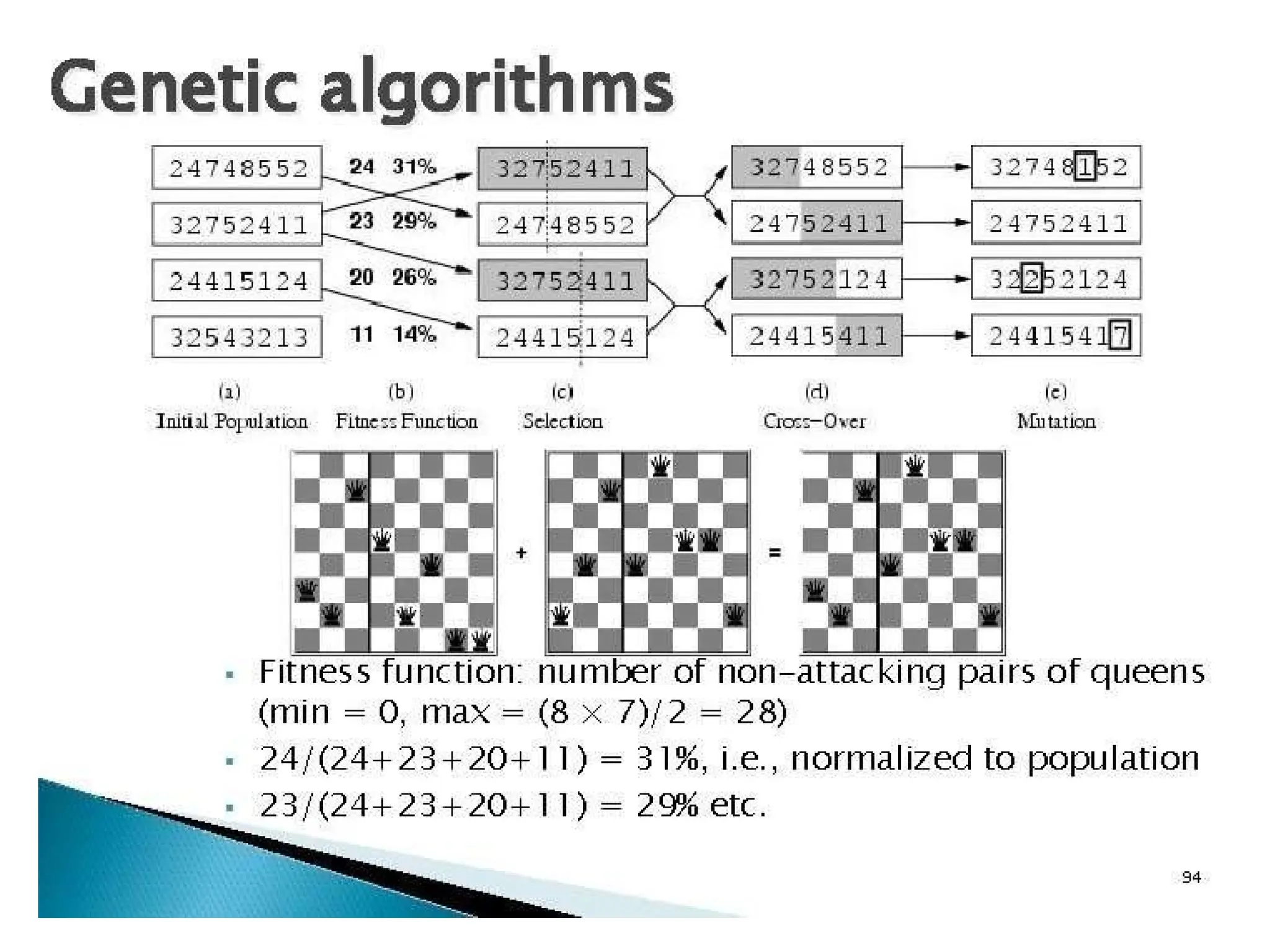
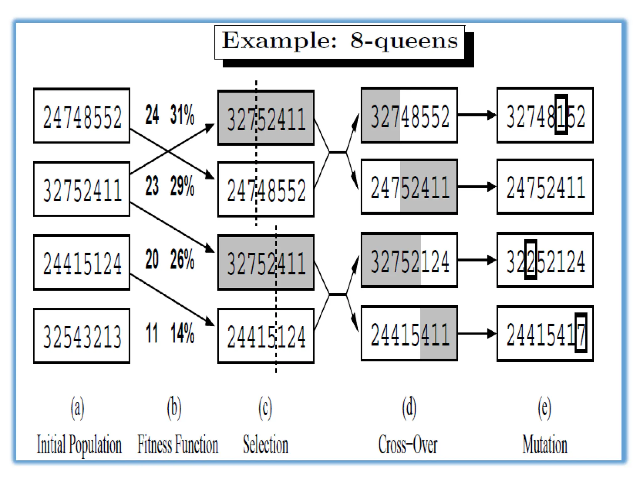
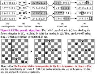
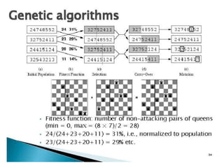
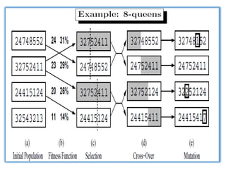
Figure 4.15 Thegenetic algorithm. The initial population in (a) is ranked by the
fitness function in (b), resulting in pairs for mating in (c). They produce offspring
in (d), which are subject to mutation in (e).
Figure 4.16 The 8-queens states corresponding to the first two parents in Figure 4.15(c)
and the first offspring in Figure 4.15(d). The shaded columns are lost in the crossover step
and the unshaded columns are retained.
122.
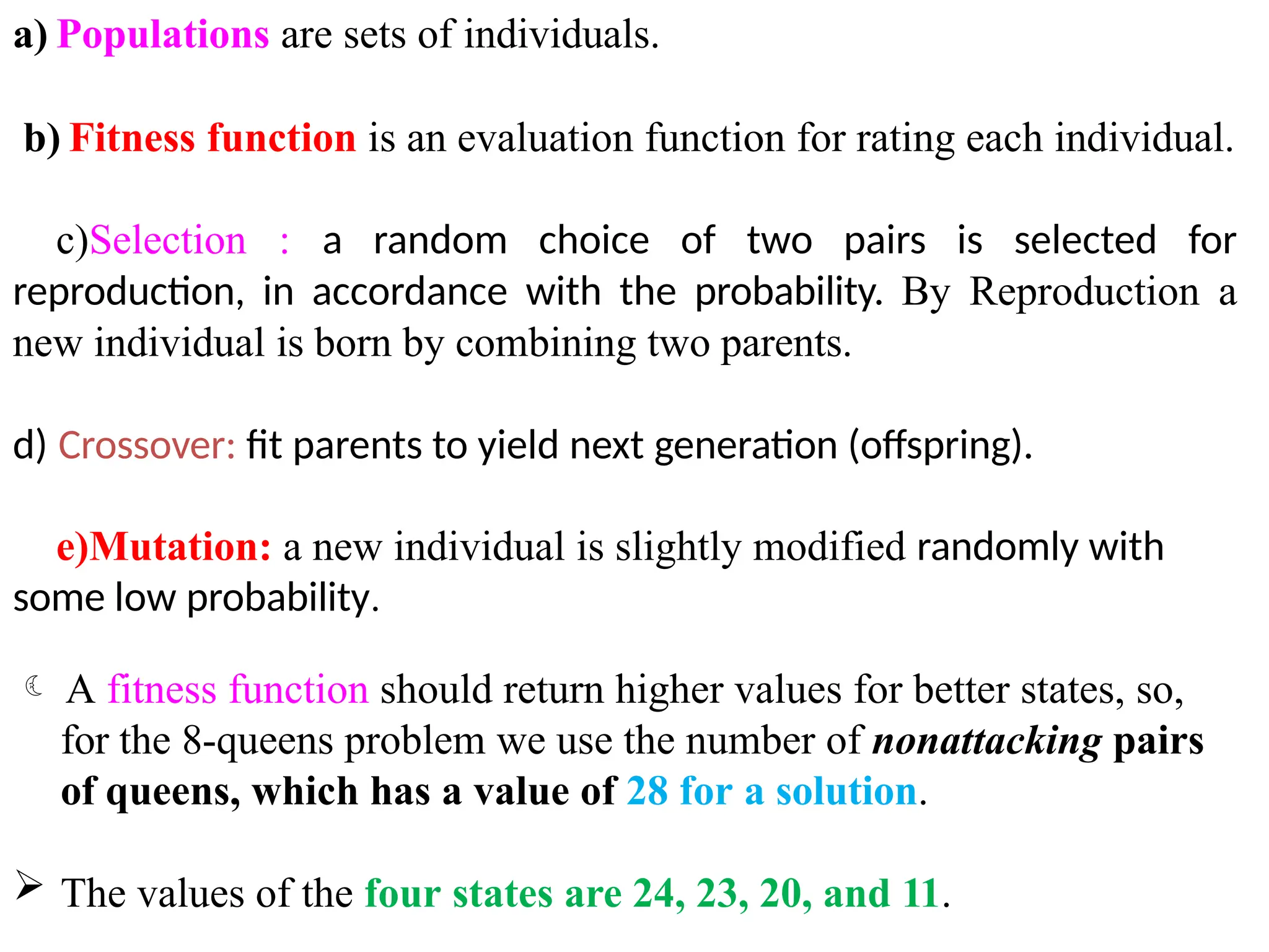
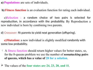
a) Populations aresets of individuals.
b) Fitness function is an evaluation function for rating each individual.
c)Selection : a random choice of two pairs is selected for
reproduction, in accordance with the probability. By Reproduction a
new individual is born by combining two parents.
d) Crossover: fit parents to yield next generation (offspring).
e)Mutation: a new individual is slightly modified randomly with
some low probability.
A fitness function should return higher values for better states, so,
for the 8-queens problem we use the number of nonattacking pairs
of queens, which has a value of 28 for a solution.
The values of the four states are 24, 23, 20, and 11.
123.
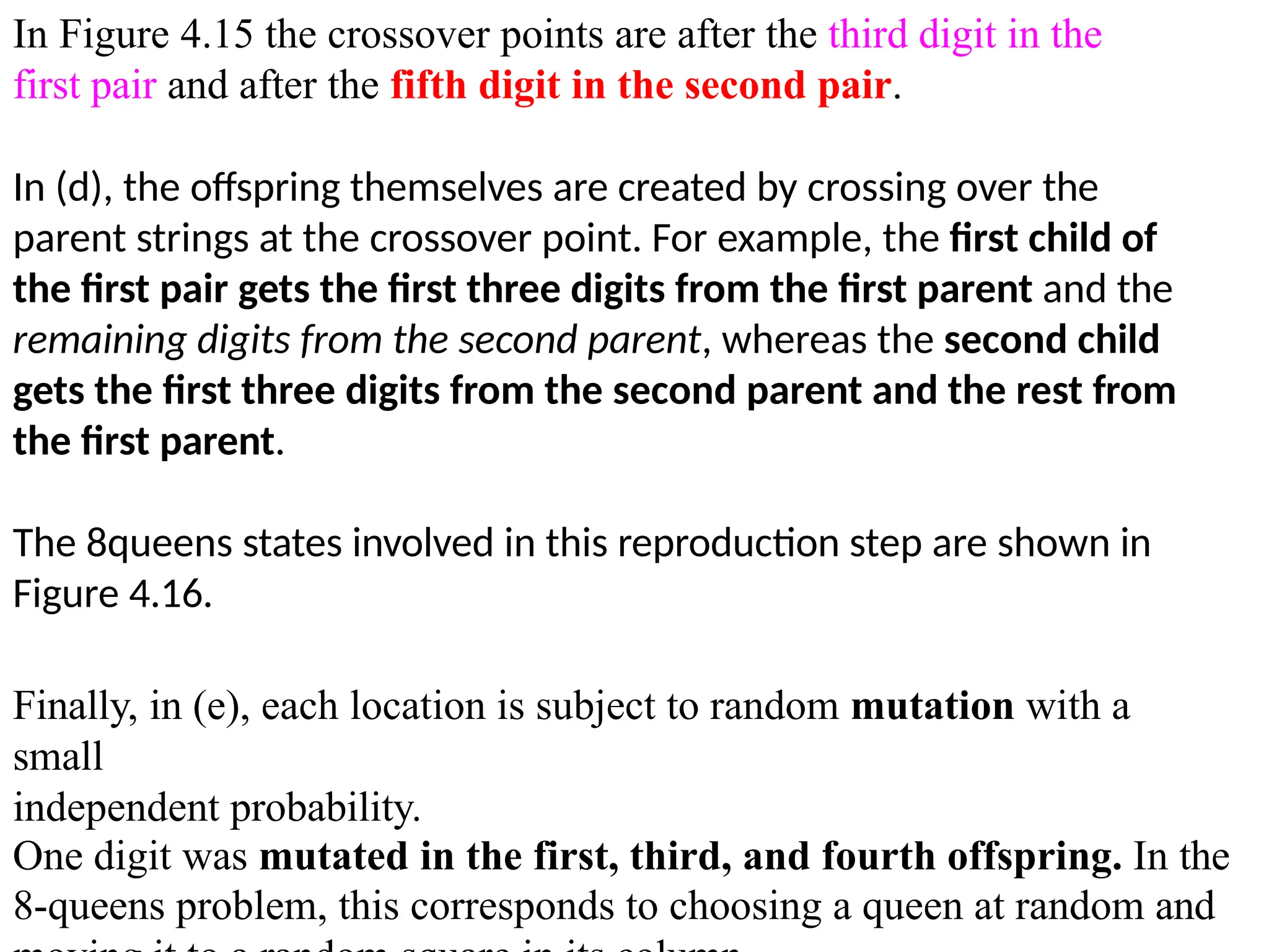
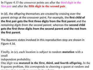
In Figure 4.15the crossover points are after the third digit in the
first pair and after the fifth digit in the second pair.
In (d), the offspring themselves are created by crossing over the
parent strings at the crossover point. For example, the first child of
the first pair gets the first three digits from the first parent and the
remaining digits from the second parent, whereas the second child
gets the first three digits from the second parent and the rest from
the first parent.
The 8queens states involved in this reproduction step are shown in
Figure 4.16.
Finally, in (e), each location is subject to random mutation with a
small
independent probability.
One digit was mutated in the first, third, and fourth offspring. In the
8-queens problem, this corresponds to choosing a queen at random and
126.
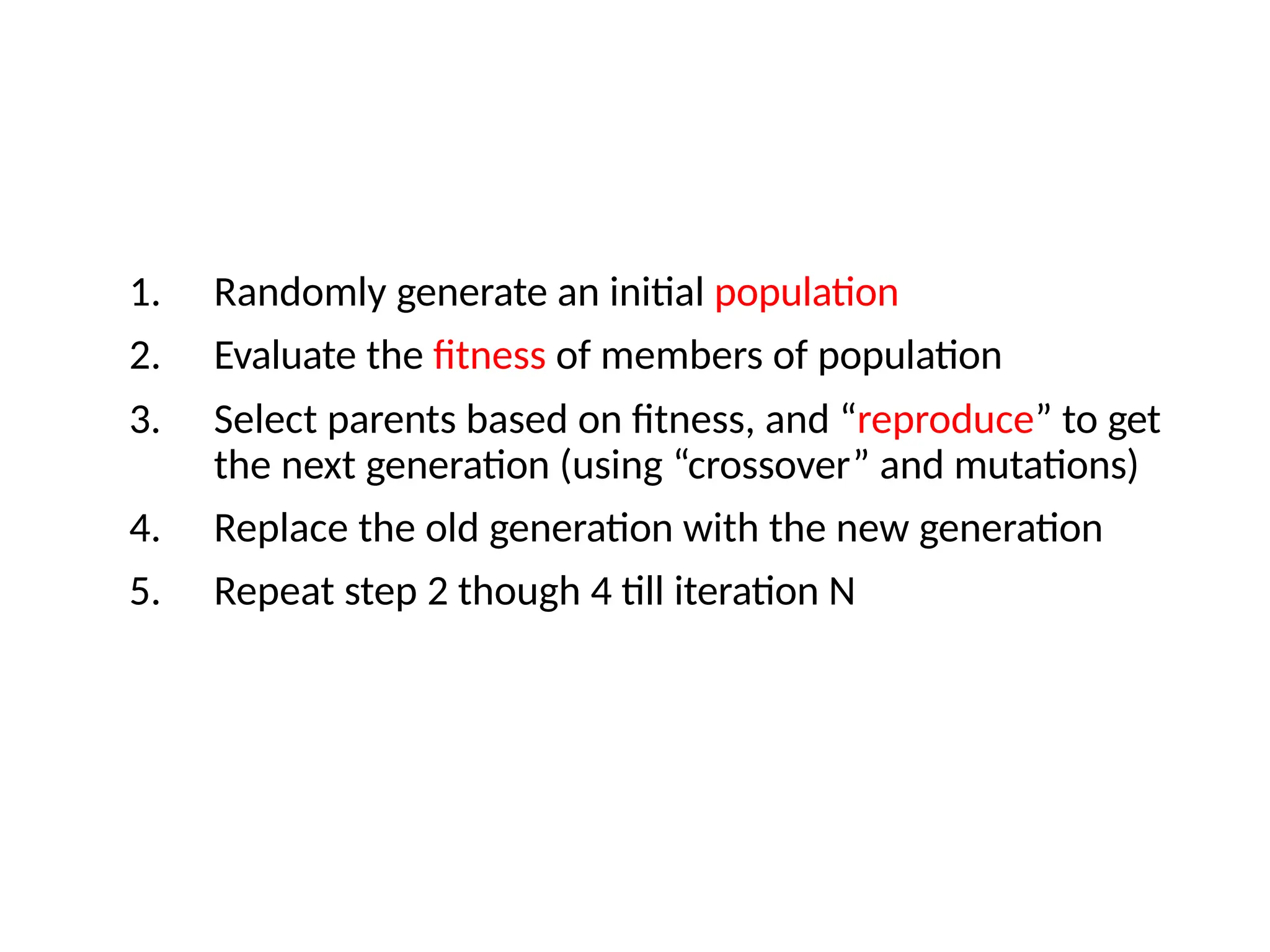
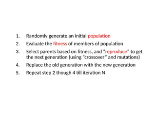
1. Randomly generatean initial population
2. Evaluate the fitness of members of population
3. Select parents based on fitness, and “reproduce” to get
the next generation (using “crossover” and mutations)
4. Replace the old generation with the new generation
5. Repeat step 2 though 4 till iteration N


![1) Hill-climbing search
It is simply a loop that continually moves in the direction of
increasing value-that is, uphill. It terminates when it reaches a
"peak" where no neighbor has a higher value.
function HILL-CLIMBING(problem) returns a state that is a local
maximum
inputs: problem, a problem
local variables: current, a node
neighbour, a node
current MAKENODE(INITIAL-STATE [problem])
loop do
neighbour a highest-valued successor of current
if Value[neighbour] <= Value[current] then return STATE [current ]
current neighbour
Figure 4.11 The hill-climbing search algorithm, which is the most basic local search
technique. At each step the current node is replaced by the best neighbor; in this
version, that means the neighbor with the highest VALUE, but if a heuristic cost](https://image.slidesharecdn.com/aiml-unit-1problemsolvingagents-250807025417-70abf994/85/AI-ML-UNIT-1-problem-solving-agents-pptx-94-320.jpg)


![1) Hill-climbing search
It is simply a loop that continually moves in the direction of
increasing value-that is, uphill. It terminates when it reaches a
"peak" where no neighbor has a higher value.
function HILL-CLIMBING(problem) returns a state that is a local
maximum
inputs: problem, a problem
local variables: current, a node
neighbour, a node
current MAKENODE(INITIAL-STATE [problem])
loop do
neighbour a highest-valued successor of current
if Value[neighbour] <= Value[current] then return STATE [current ]
current neighbour
Figure 4.11 The hill-climbing search algorithm, which is the most basic local search
technique. At each step the current node is replaced by the best neighbor; in this
version, that means the neighbor with the highest VALUE, but if a heuristic cost](https://image.slidesharecdn.com/aiml-unit-1problemsolvingagents-250807025417-70abf994/75/AI-ML-UNIT-1-problem-solving-agents-pptx-94-2048.jpg)