Downloaded 498 times


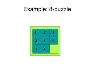
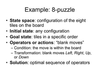
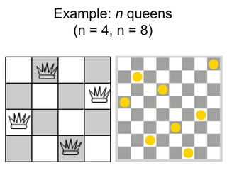
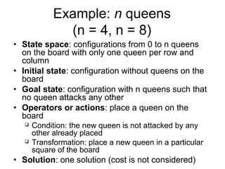
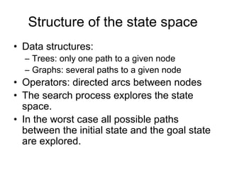


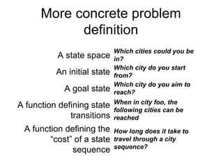
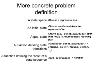


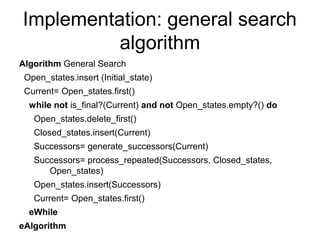
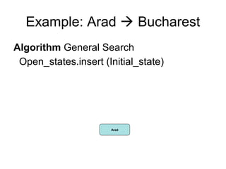
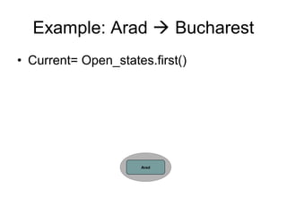
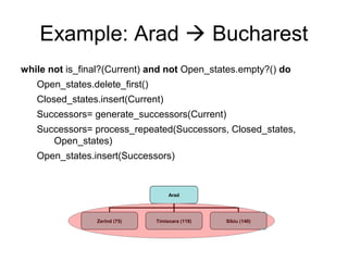

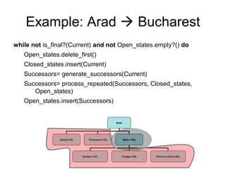
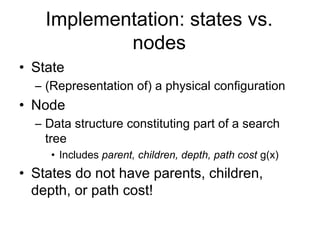

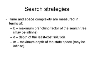
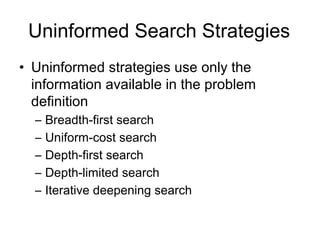
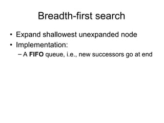


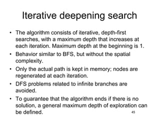
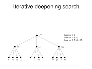

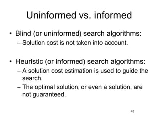


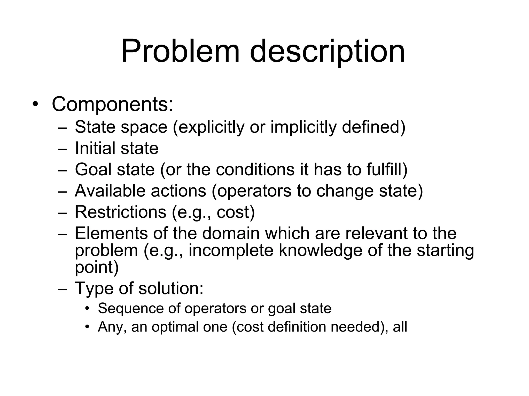
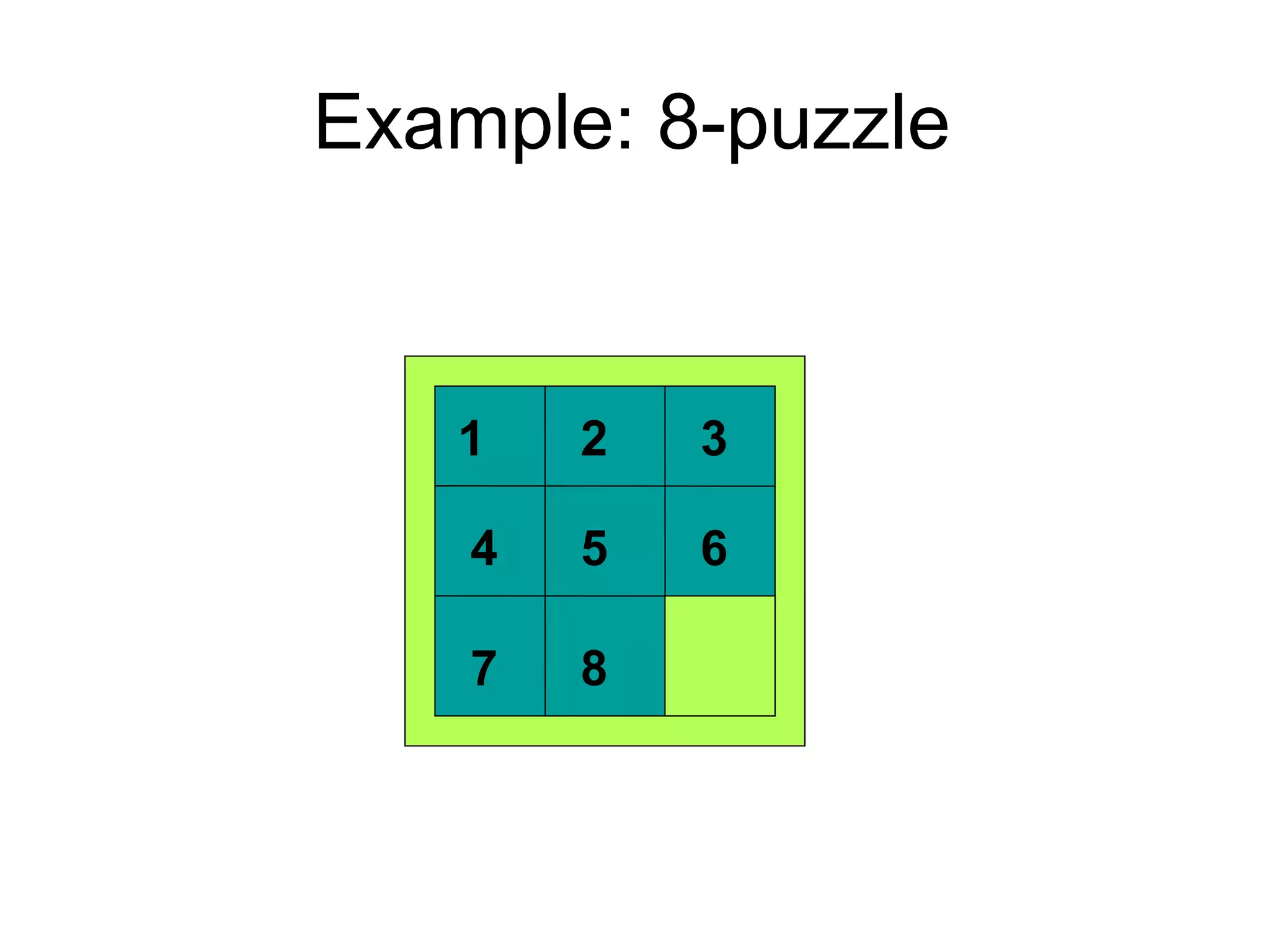
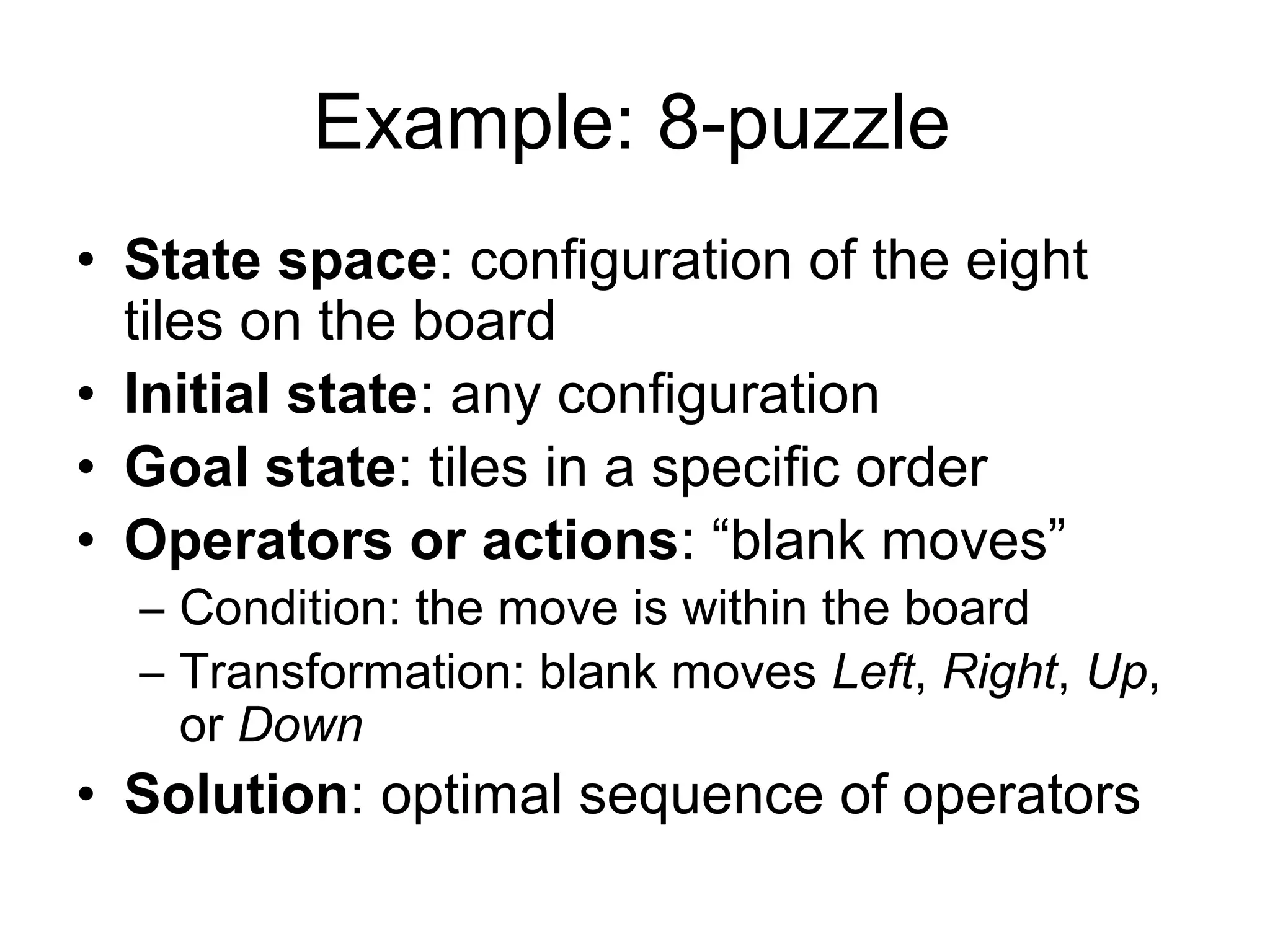
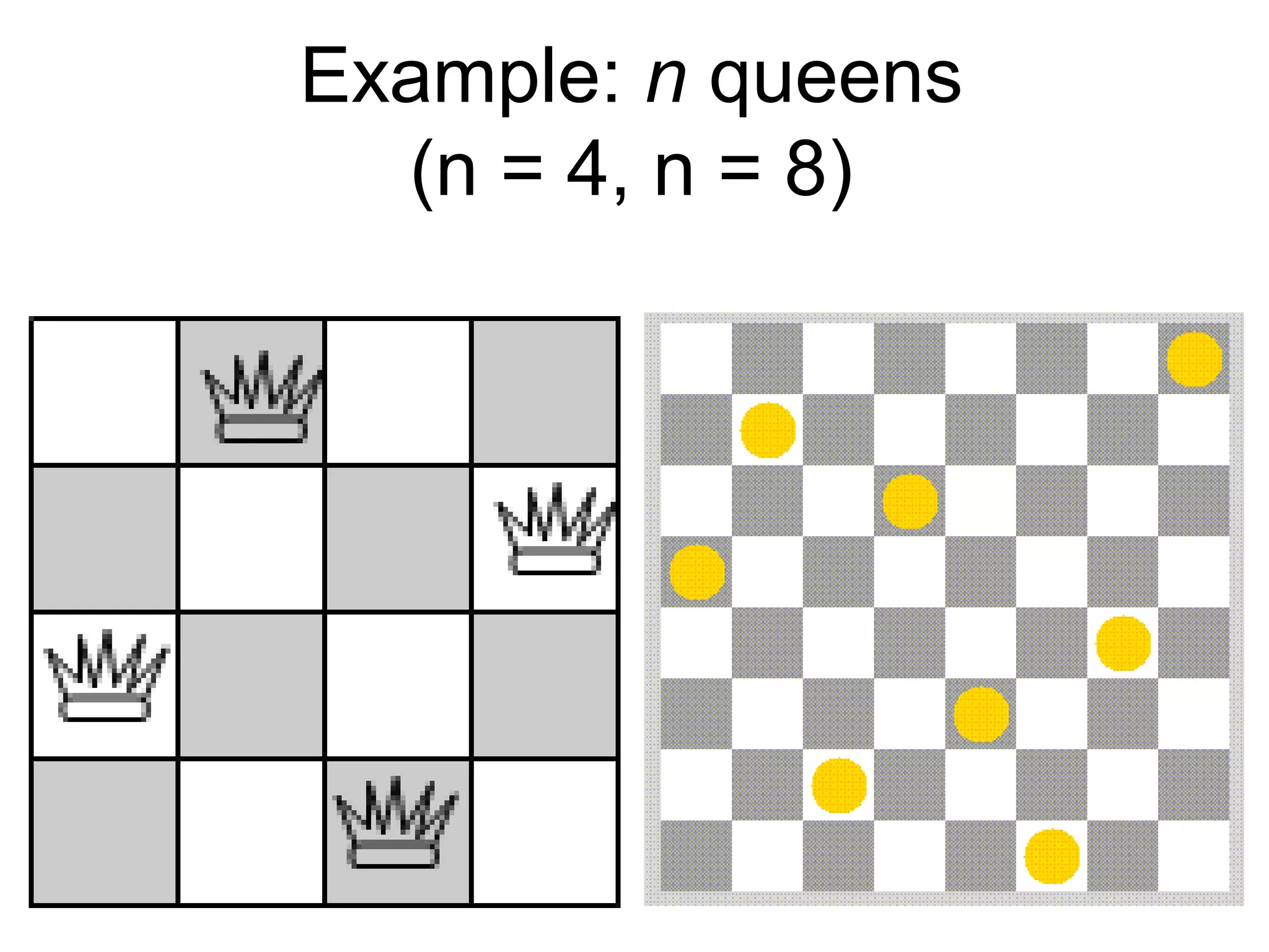


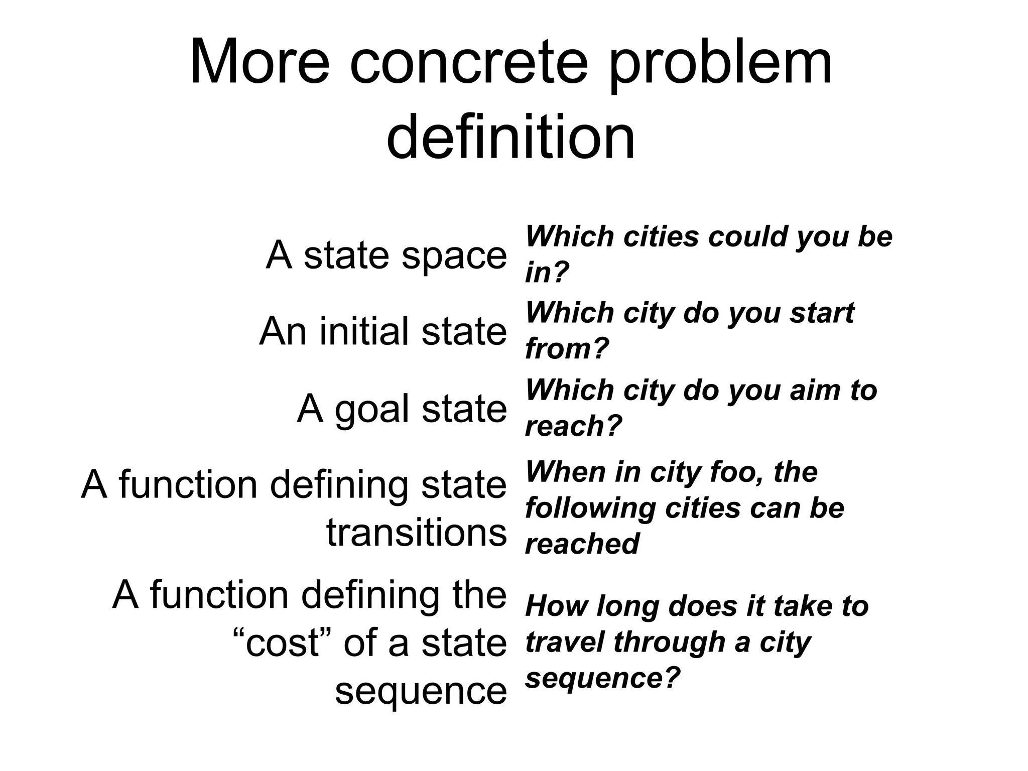

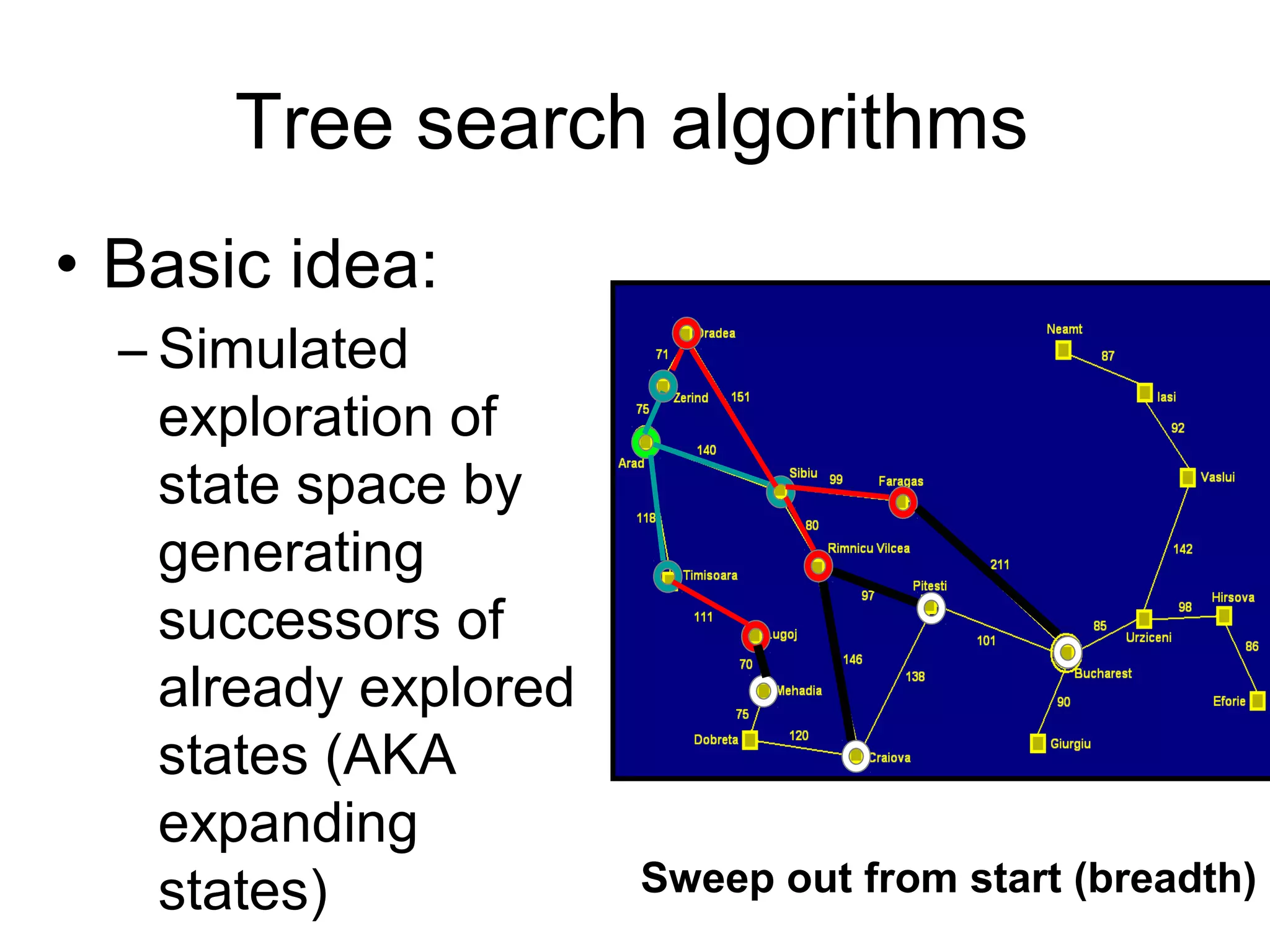
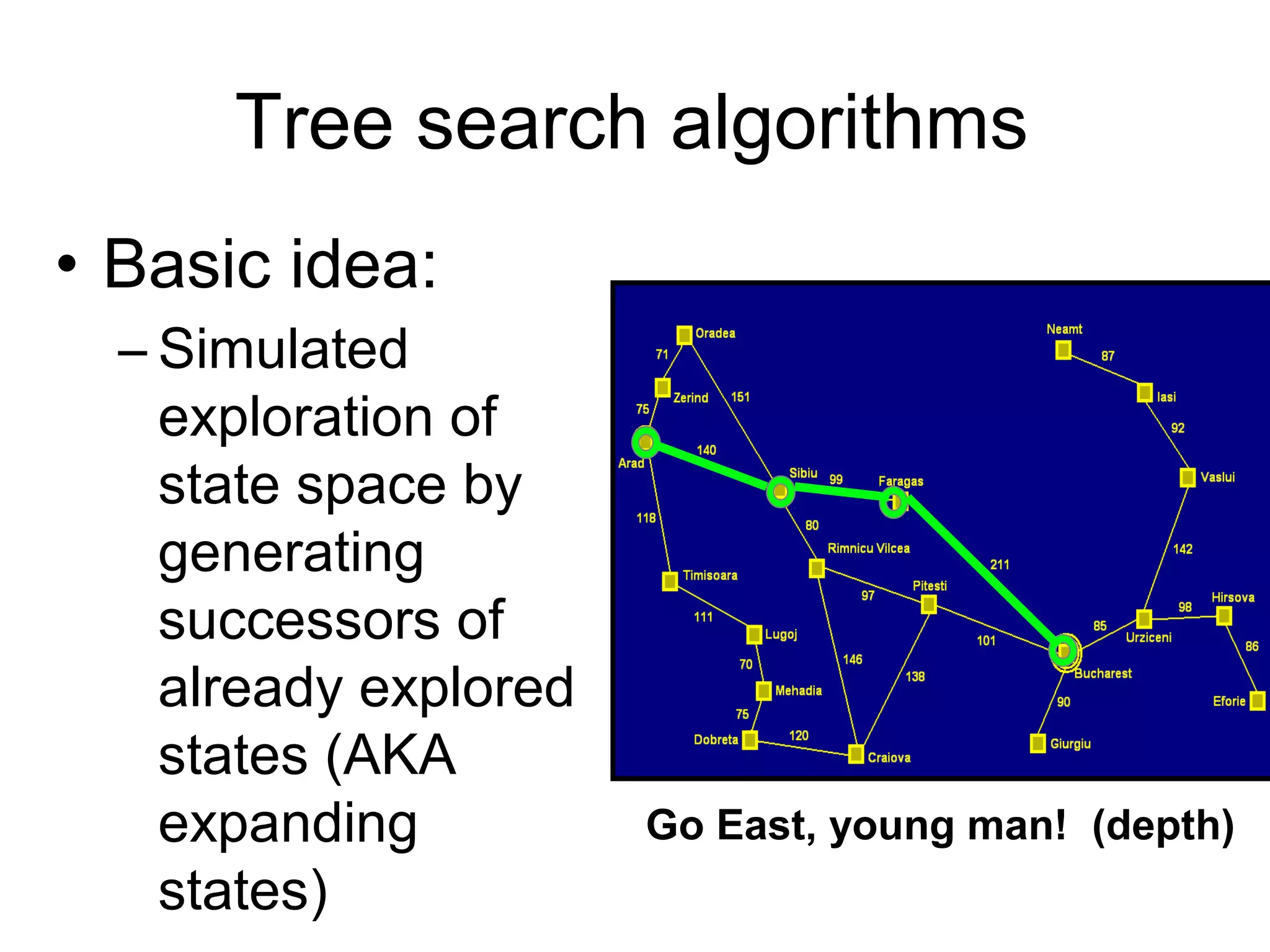
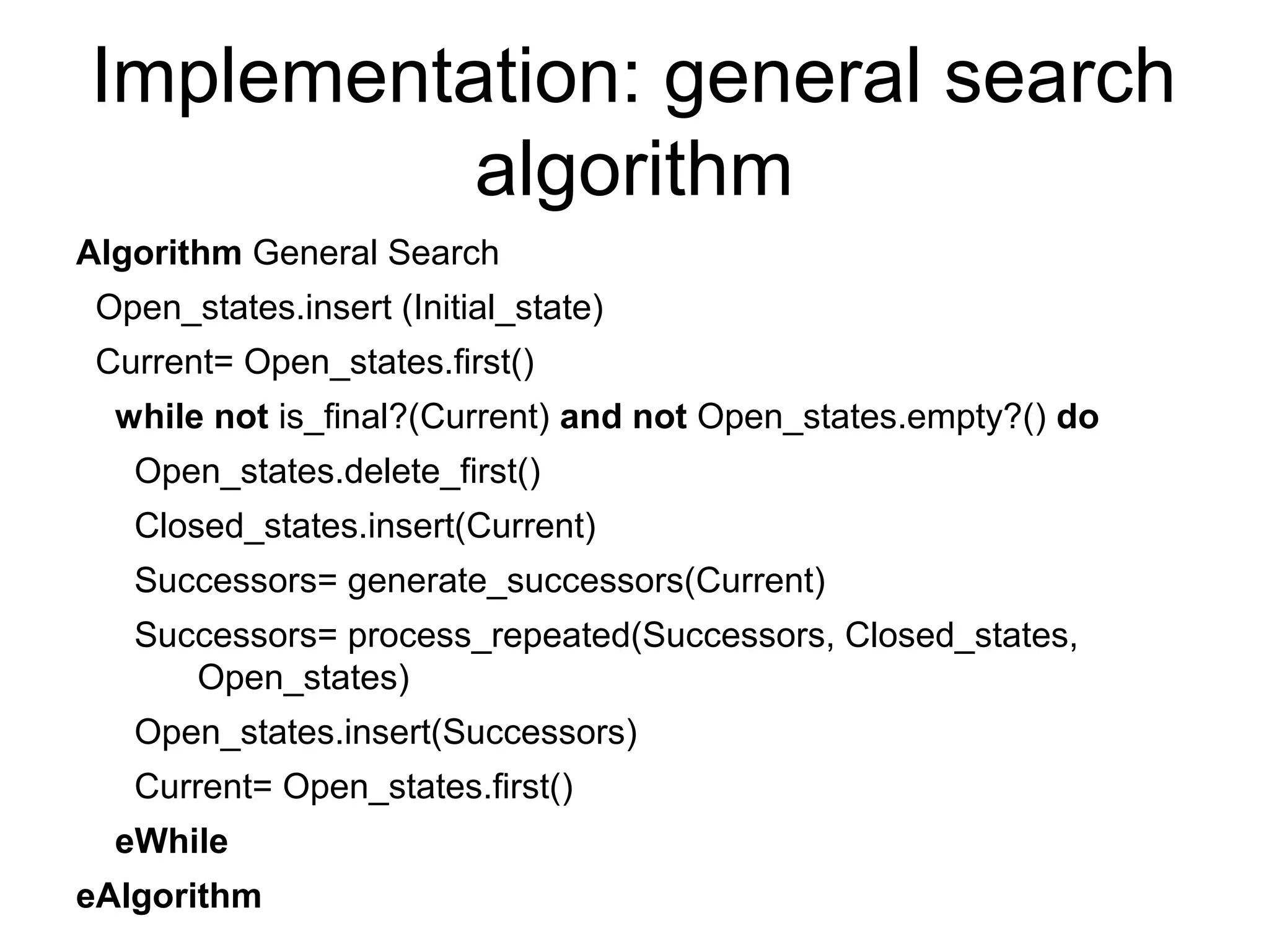


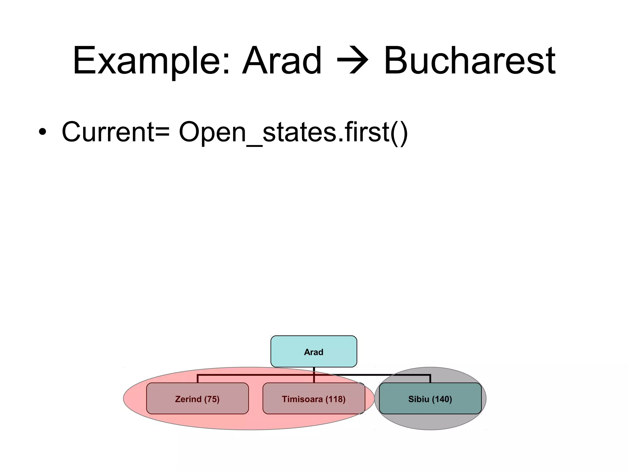


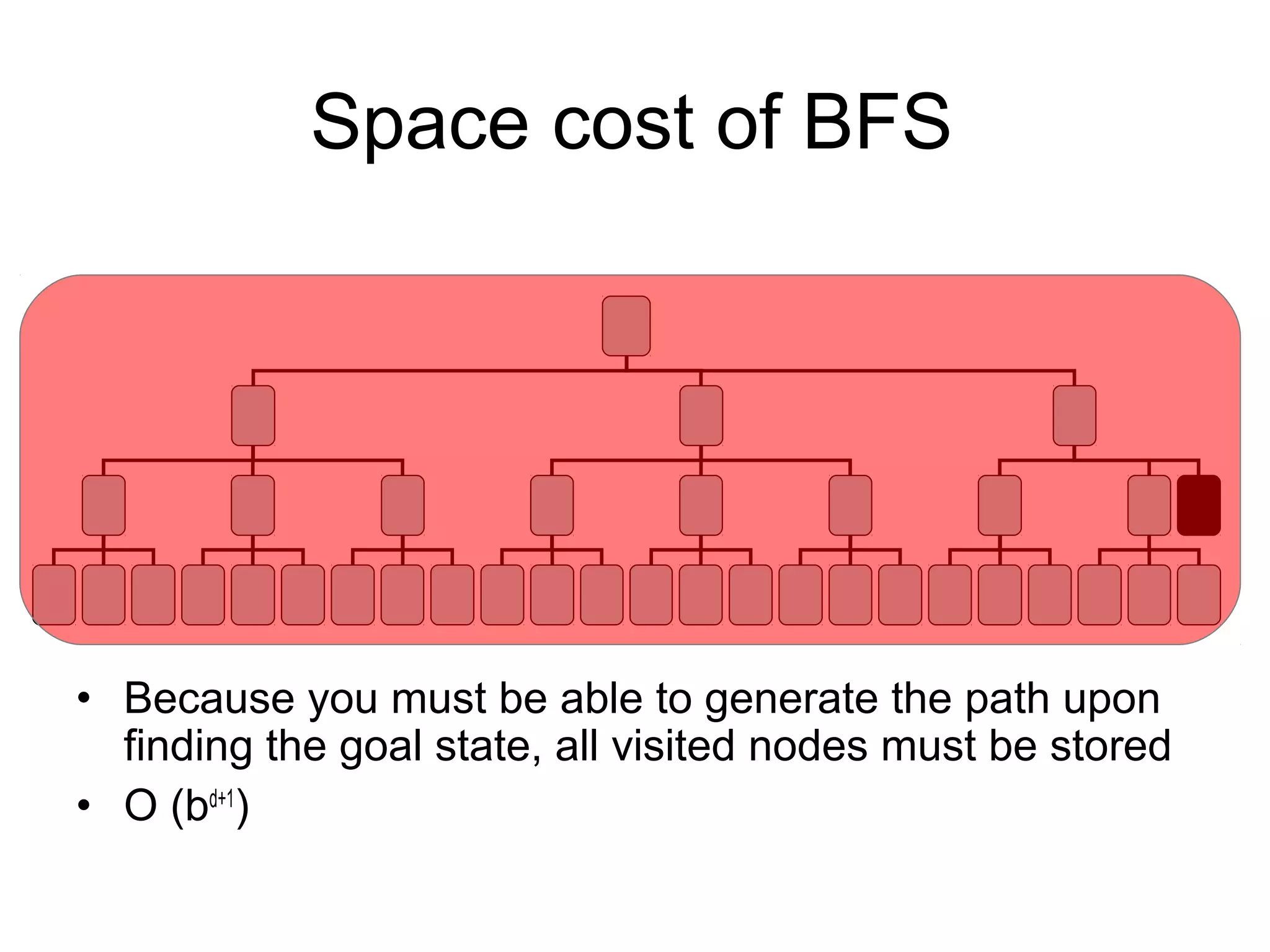


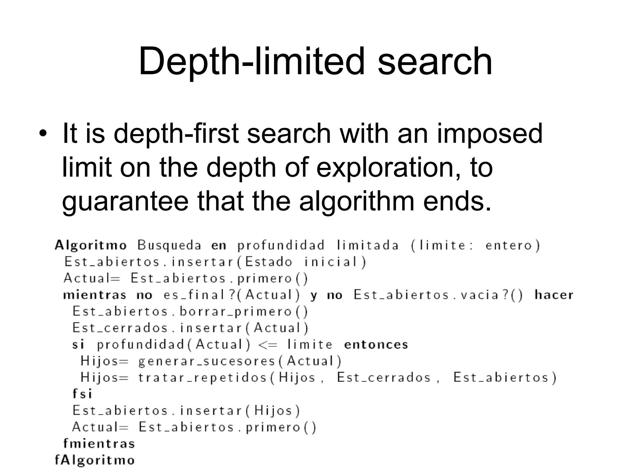

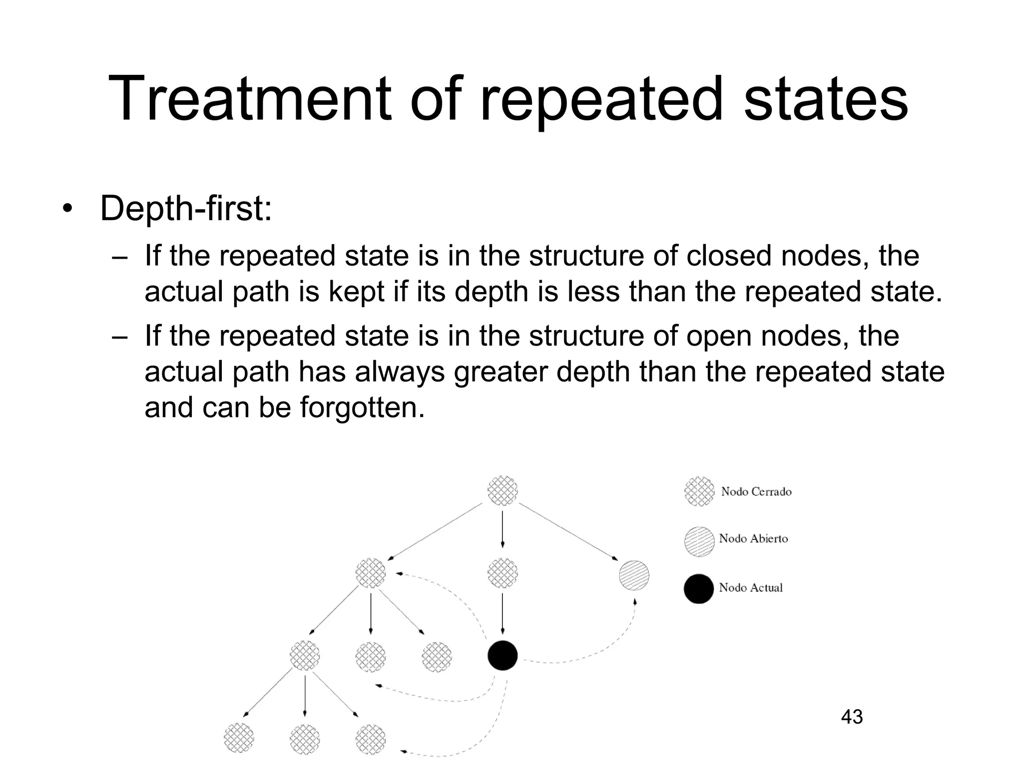
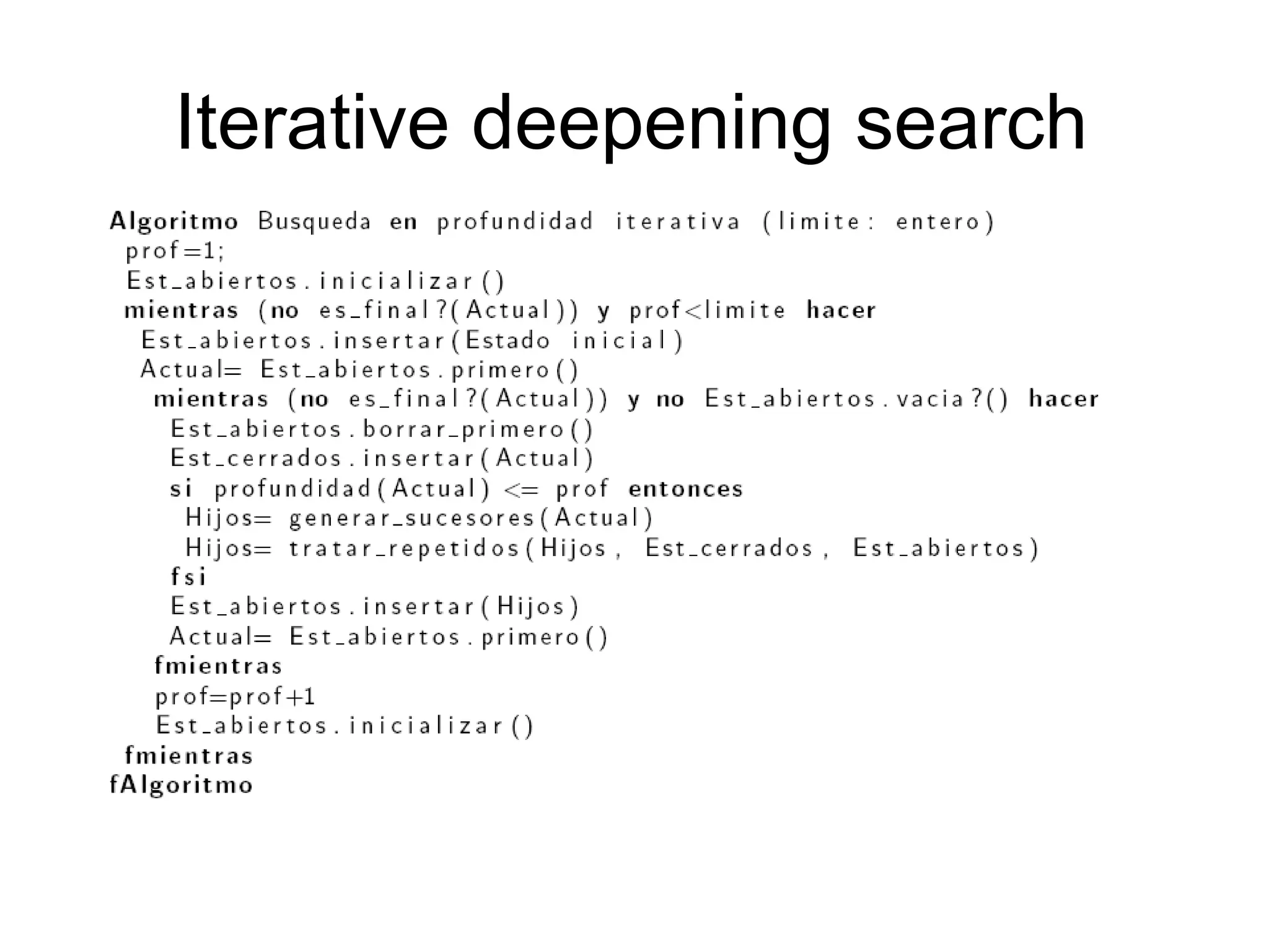


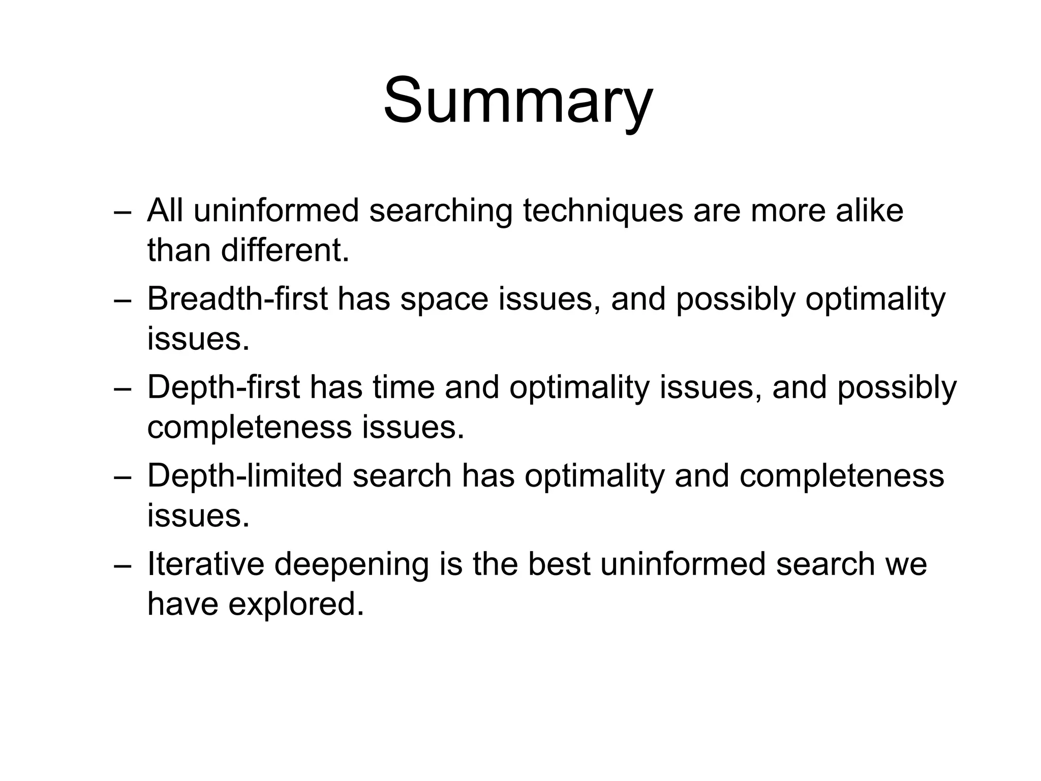

Artificial Intelligence involves representing problems as state spaces and using algorithms to search the state space to solve the problem. The document discusses key concepts in problem solving using search including representing the problem as states, defining state transitions with successor functions, and exploring the resulting state space to find a solution. It provides examples of representing common problems like the 8-puzzle and n-queens as state spaces. The document also summarizes uninformed search strategies like breadth-first, depth-first, and iterative deepening search that use the problem definition to search the state space without using heuristics.


