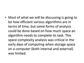
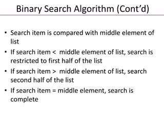
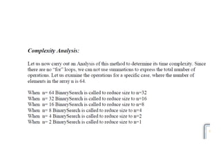
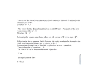
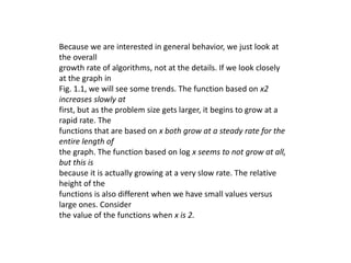
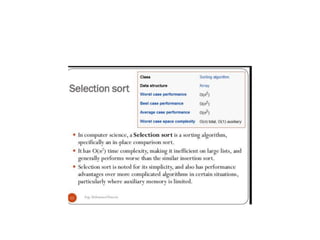
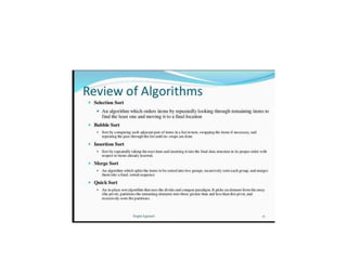
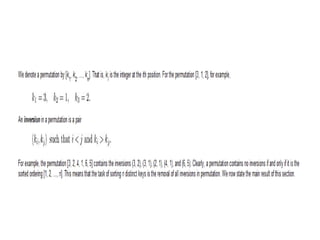
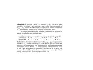
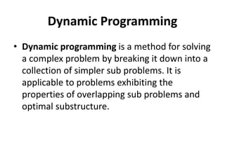
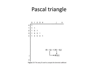
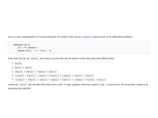
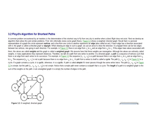
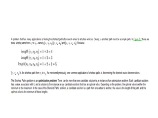
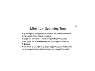
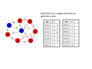
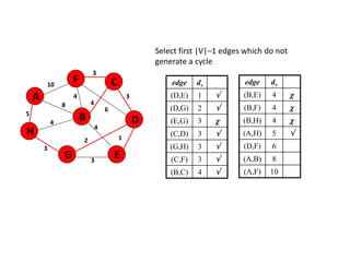
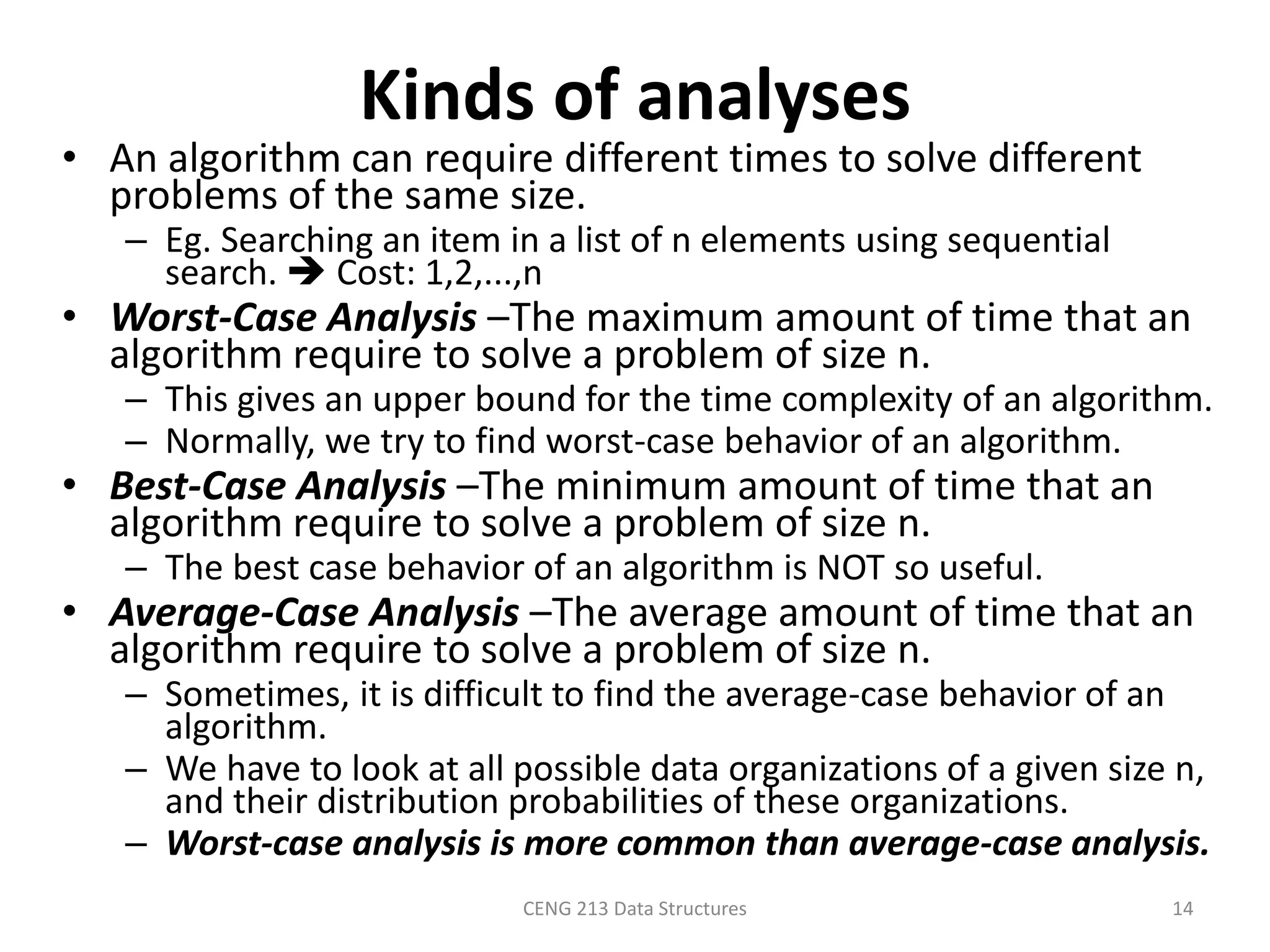
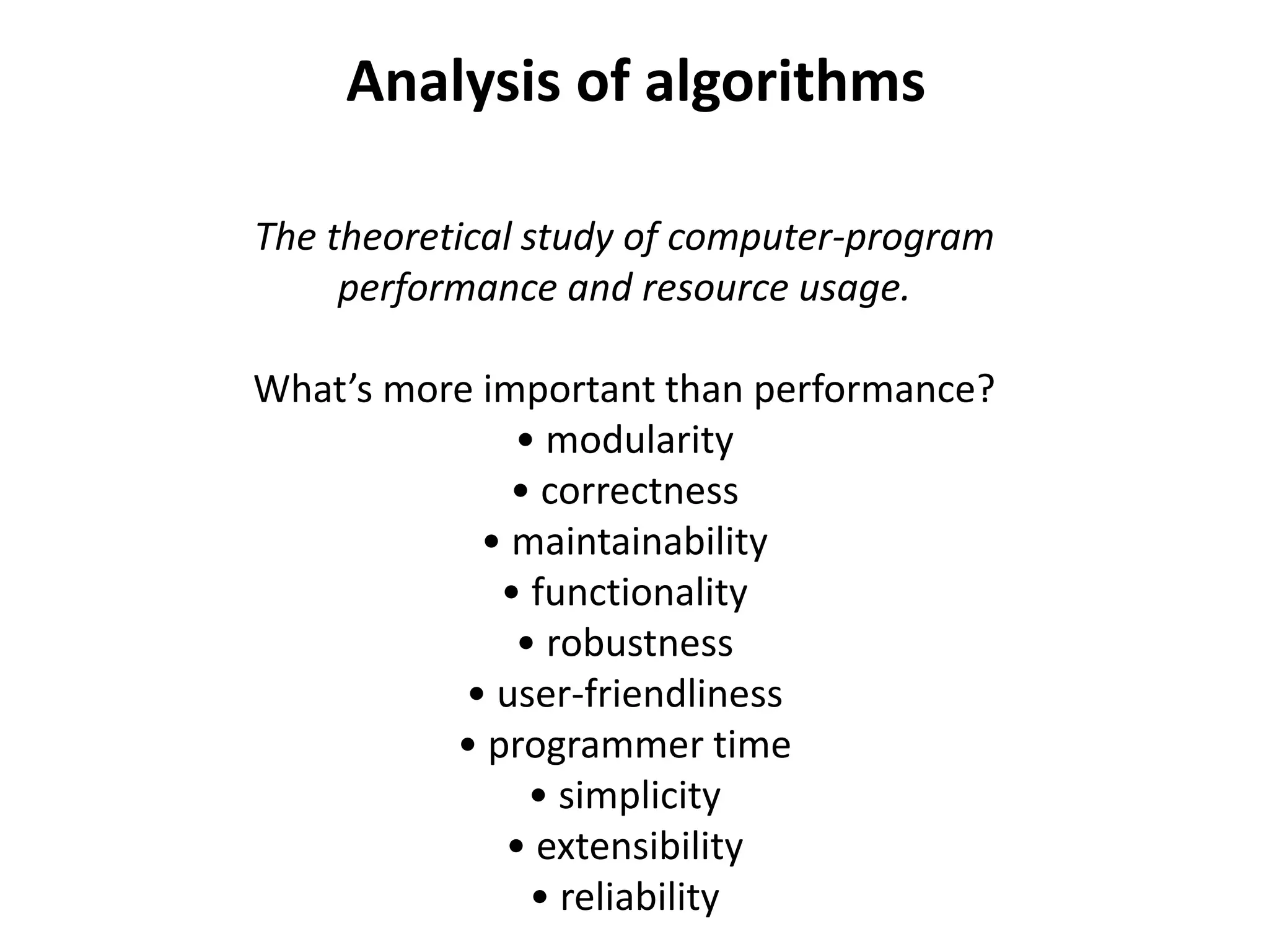
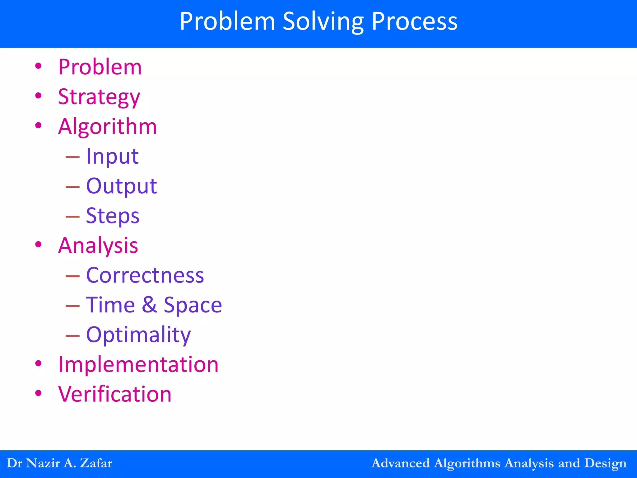
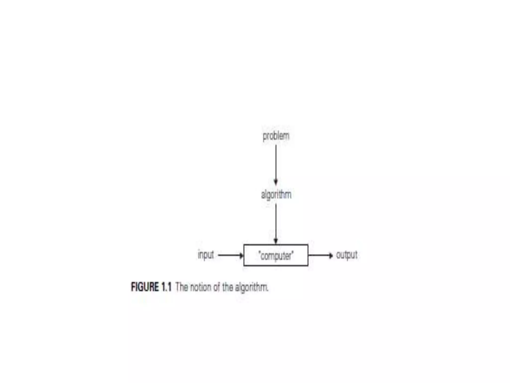
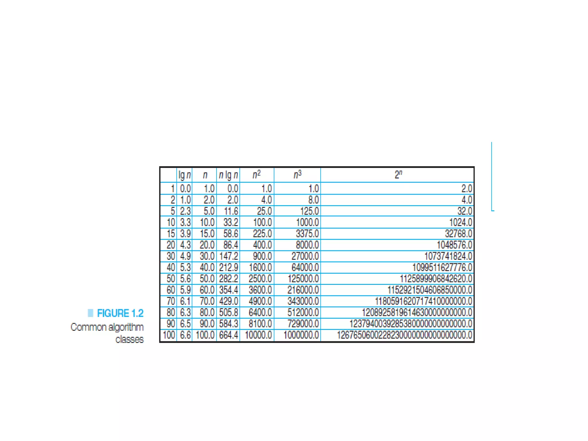
The document provides an overview of algorithms, emphasizing their definition as step-by-step procedures for problem-solving, and discusses data structures that enable efficient data management. It explains various analyses of algorithms such as worst-case, best-case, and average-case performance to evaluate efficiency in terms of time and space complexity, along with examples of sorting and searching algorithms. Additionally, it touches on more advanced concepts like dynamic programming and greedy algorithms, underlining the importance of selecting appropriate algorithms based on their efficiency and suitability for specific tasks.


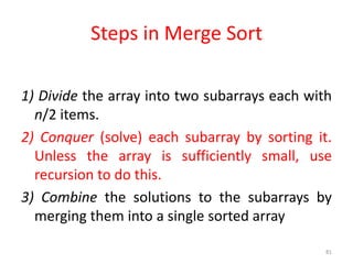
![Algorithm for finding maximum
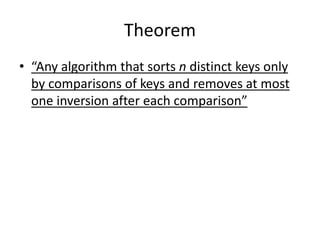
number in an array
Algorithm arrayMax(A, n)
Input array A of n integers
Output maximum element of A
currentMax A[0]
for i 1 to n 1 do
if A[i] currentMax then
currentMax A[i]
return currentMax](https://image.slidesharecdn.com/algorithmanalysis-150906142919-lva1-app6892/85/Algorithm-analysis-All-in-one-17-320.jpg)

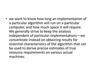
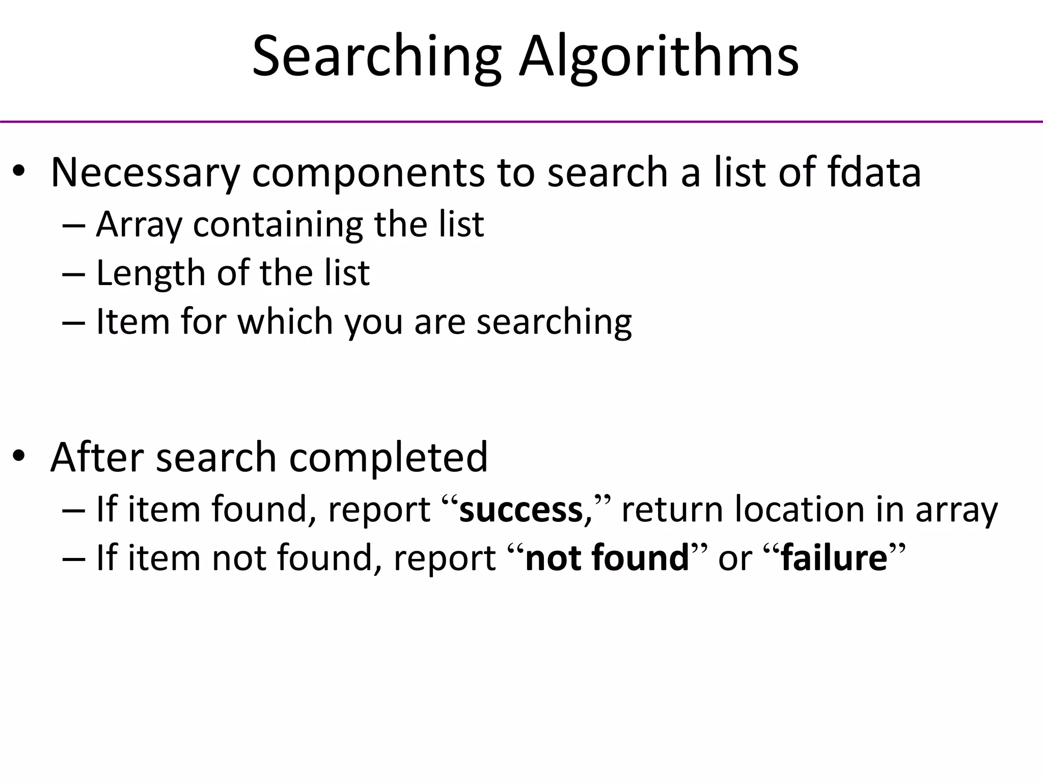
![• Suppose that you want to determine whether 27 is in the list
• First compare 27 with list[0]; that is, compare 27 with
35
• Because list[0] ≠ 27, you then compare 27 with
list[1]
• Because list[1] ≠ 27, you compare 27 with the next
element in the list
• Because list[2] = 27, the search stops
• This search is successful!
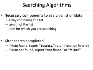
Searching Algorithms (Cont’d)
Figure 1: Array list with seven (07) elements](https://image.slidesharecdn.com/algorithmanalysis-150906142919-lva1-app6892/85/Algorithm-analysis-All-in-one-21-320.jpg)
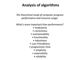
![• Let’s now search for 10
• The search starts at the first element in the list; that
is, at list[0]
• Proceeding as before, we see that this time the
search item, which is 10, is compared with every
item in the list
• Eventually, no more data is left in the list to compare
with the search item; this is an unsuccessful search
Searching Algorithms (Cont’d)](https://image.slidesharecdn.com/algorithmanalysis-150906142919-lva1-app6892/85/Algorithm-analysis-All-in-one-22-320.jpg)
![Algorithm of Sequential Searching
• The complete algorithm for sequential search is
//list the elements to be searched
//target the value being searched for
//N the number of elements in the list
SequentialSearch( list, target, N )
• for i = 1 to N do
• if (target = list[i])
• return i
• end if
• end for
• return 0](https://image.slidesharecdn.com/algorithmanalysis-150906142919-lva1-app6892/85/Algorithm-analysis-All-in-one-23-320.jpg)
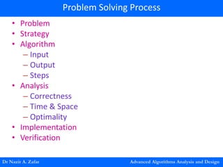
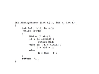
![• Determine whether 75 is in the list
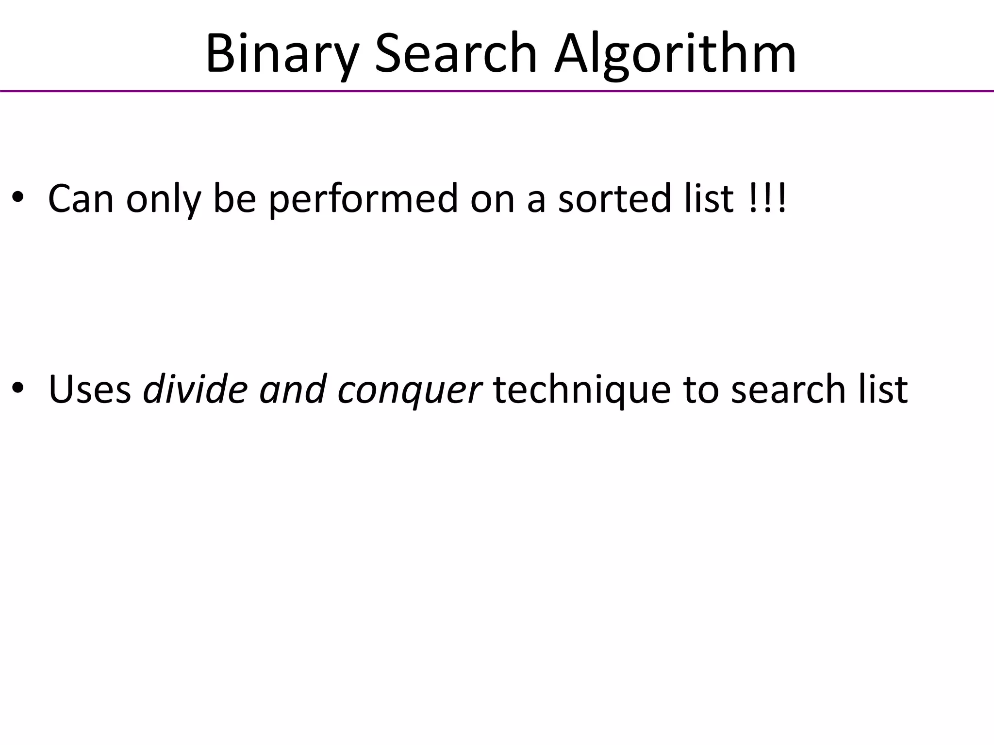
Binary Search Algorithm (Cont’d)
Figure 2: Array list with twelve (12) elements
Figure 3: Search list, list[0] … list[11]](https://image.slidesharecdn.com/algorithmanalysis-150906142919-lva1-app6892/85/Algorithm-analysis-All-in-one-27-320.jpg)
![Binary Search Algorithm (Cont’d)
Figure 4: Search list, list[6] … list[11]](https://image.slidesharecdn.com/algorithmanalysis-150906142919-lva1-app6892/85/Algorithm-analysis-All-in-one-28-320.jpg)

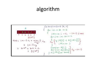
![Algorithm
• MIN(A,K,N,LOC)
• 1. Set MIN=A[K] and LOC=K
• Repeat for J=K+1,K+2…….N
• If MIN>A[J], then Set MIN=A[J] and LOC=J.
• Interchange A[K] and A[LOC].
• Exit](https://image.slidesharecdn.com/algorithmanalysis-150906142919-lva1-app6892/85/Algorithm-analysis-All-in-one-71-320.jpg)


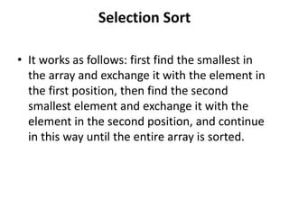
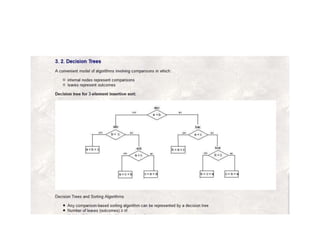
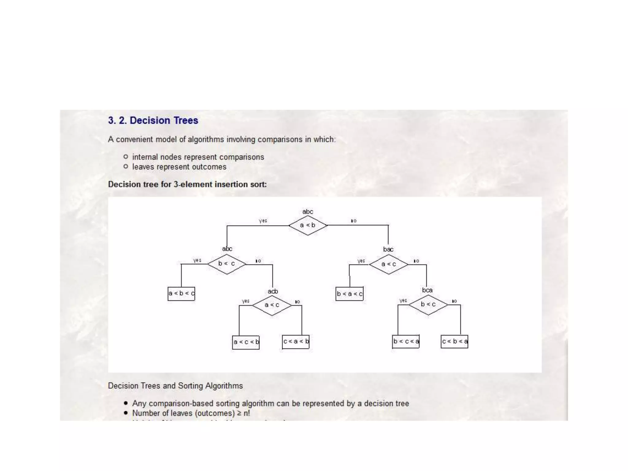
![Decision Trees for Sorting Algorithms
• Void sortthree(keytype S[])
• {
• Keytype a,b,c;
• a=S[1]; b= S[2]; c= S[3];
• If(a<b)
• If(b<c)
• S=a,b,c
• Else if (a<c)
• S=a,c,b;
• Else
• S=c,a,b;
• Else if (b<c)
• If (a<c)
• S= b,a,c;
• Else
• S= b,c,a;
• Else
• S=c,b,a;
• }](https://image.slidesharecdn.com/algorithmanalysis-150906142919-lva1-app6892/85/Algorithm-analysis-All-in-one-87-320.jpg)

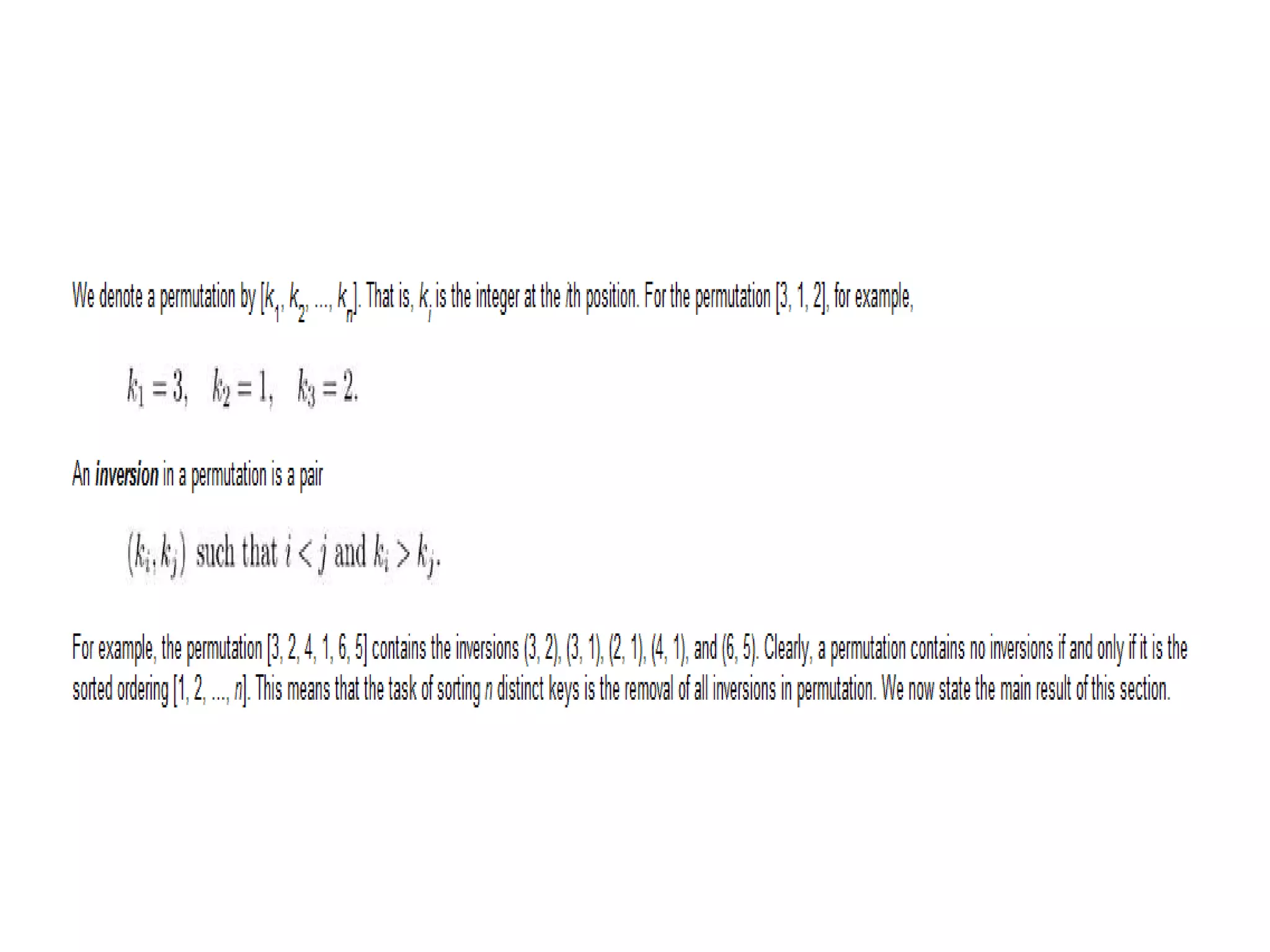
![Proof
• Suppose that currently the array S contains the
permutation [2, 4, 3, 1] and we are comparing 2
with 1. After that comparison, 2 and 1 will be
exchanged, thereby removing the inversions
(2, 1), (4, 1), and (3, 1). However, the inversions (4,
2) and (3, 2) have been added, and the net
reduction, in inversions is only one. This example
illustrates the general result that Exchange Sort
always has a net reduction of at most one
inversion after each comparison.](https://image.slidesharecdn.com/algorithmanalysis-150906142919-lva1-app6892/85/Algorithm-analysis-All-in-one-97-320.jpg)


![Algorithm for finding maximum
number in an array
Algorithm arrayMax(A, n)
Input array A of n integers
Output maximum element of A
currentMax A[0]
for i 1 to n 1 do
if A[i] currentMax then
currentMax A[i]
return currentMax](https://image.slidesharecdn.com/algorithmanalysis-150906142919-lva1-app6892/75/Algorithm-analysis-All-in-one-17-2048.jpg)

![• Suppose that you want to determine whether 27 is in the list
• First compare 27 with list[0]; that is, compare 27 with
35
• Because list[0] ≠ 27, you then compare 27 with
list[1]
• Because list[1] ≠ 27, you compare 27 with the next
element in the list
• Because list[2] = 27, the search stops
• This search is successful!
Searching Algorithms (Cont’d)
Figure 1: Array list with seven (07) elements](https://image.slidesharecdn.com/algorithmanalysis-150906142919-lva1-app6892/75/Algorithm-analysis-All-in-one-21-2048.jpg)
![• Let’s now search for 10
• The search starts at the first element in the list; that
is, at list[0]
• Proceeding as before, we see that this time the
search item, which is 10, is compared with every
item in the list
• Eventually, no more data is left in the list to compare
with the search item; this is an unsuccessful search
Searching Algorithms (Cont’d)](https://image.slidesharecdn.com/algorithmanalysis-150906142919-lva1-app6892/75/Algorithm-analysis-All-in-one-22-2048.jpg)
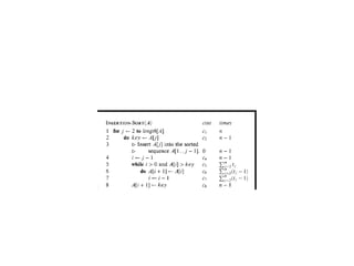
![Algorithm of Sequential Searching
• The complete algorithm for sequential search is
//list the elements to be searched
//target the value being searched for
//N the number of elements in the list
SequentialSearch( list, target, N )
• for i = 1 to N do
• if (target = list[i])
• return i
• end if
• end for
• return 0](https://image.slidesharecdn.com/algorithmanalysis-150906142919-lva1-app6892/75/Algorithm-analysis-All-in-one-23-2048.jpg)

![• Determine whether 75 is in the list
Binary Search Algorithm (Cont’d)
Figure 2: Array list with twelve (12) elements
Figure 3: Search list, list[0] … list[11]](https://image.slidesharecdn.com/algorithmanalysis-150906142919-lva1-app6892/75/Algorithm-analysis-All-in-one-27-2048.jpg)
![Binary Search Algorithm (Cont’d)
Figure 4: Search list, list[6] … list[11]](https://image.slidesharecdn.com/algorithmanalysis-150906142919-lva1-app6892/75/Algorithm-analysis-All-in-one-28-2048.jpg)


![Algorithm
• MIN(A,K,N,LOC)
• 1. Set MIN=A[K] and LOC=K
• Repeat for J=K+1,K+2…….N
• If MIN>A[J], then Set MIN=A[J] and LOC=J.
• Interchange A[K] and A[LOC].
• Exit](https://image.slidesharecdn.com/algorithmanalysis-150906142919-lva1-app6892/75/Algorithm-analysis-All-in-one-71-2048.jpg)


![Decision Trees for Sorting Algorithms
• Void sortthree(keytype S[])
• {
• Keytype a,b,c;
• a=S[1]; b= S[2]; c= S[3];
• If(a<b)
• If(b<c)
• S=a,b,c
• Else if (a<c)
• S=a,c,b;
• Else
• S=c,a,b;
• Else if (b<c)
• If (a<c)
• S= b,a,c;
• Else
• S= b,c,a;
• Else
• S=c,b,a;
• }](https://image.slidesharecdn.com/algorithmanalysis-150906142919-lva1-app6892/75/Algorithm-analysis-All-in-one-87-2048.jpg)


![Proof
• Suppose that currently the array S contains the
permutation [2, 4, 3, 1] and we are comparing 2
with 1. After that comparison, 2 and 1 will be
exchanged, thereby removing the inversions
(2, 1), (4, 1), and (3, 1). However, the inversions (4,
2) and (3, 2) have been added, and the net
reduction, in inversions is only one. This example
illustrates the general result that Exchange Sort
always has a net reduction of at most one
inversion after each comparison.](https://image.slidesharecdn.com/algorithmanalysis-150906142919-lva1-app6892/75/Algorithm-analysis-All-in-one-97-2048.jpg)