1
What is analgorithm?
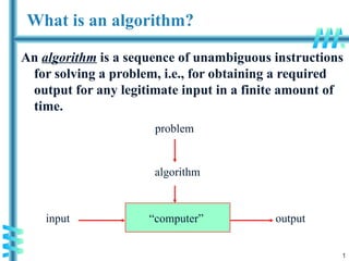
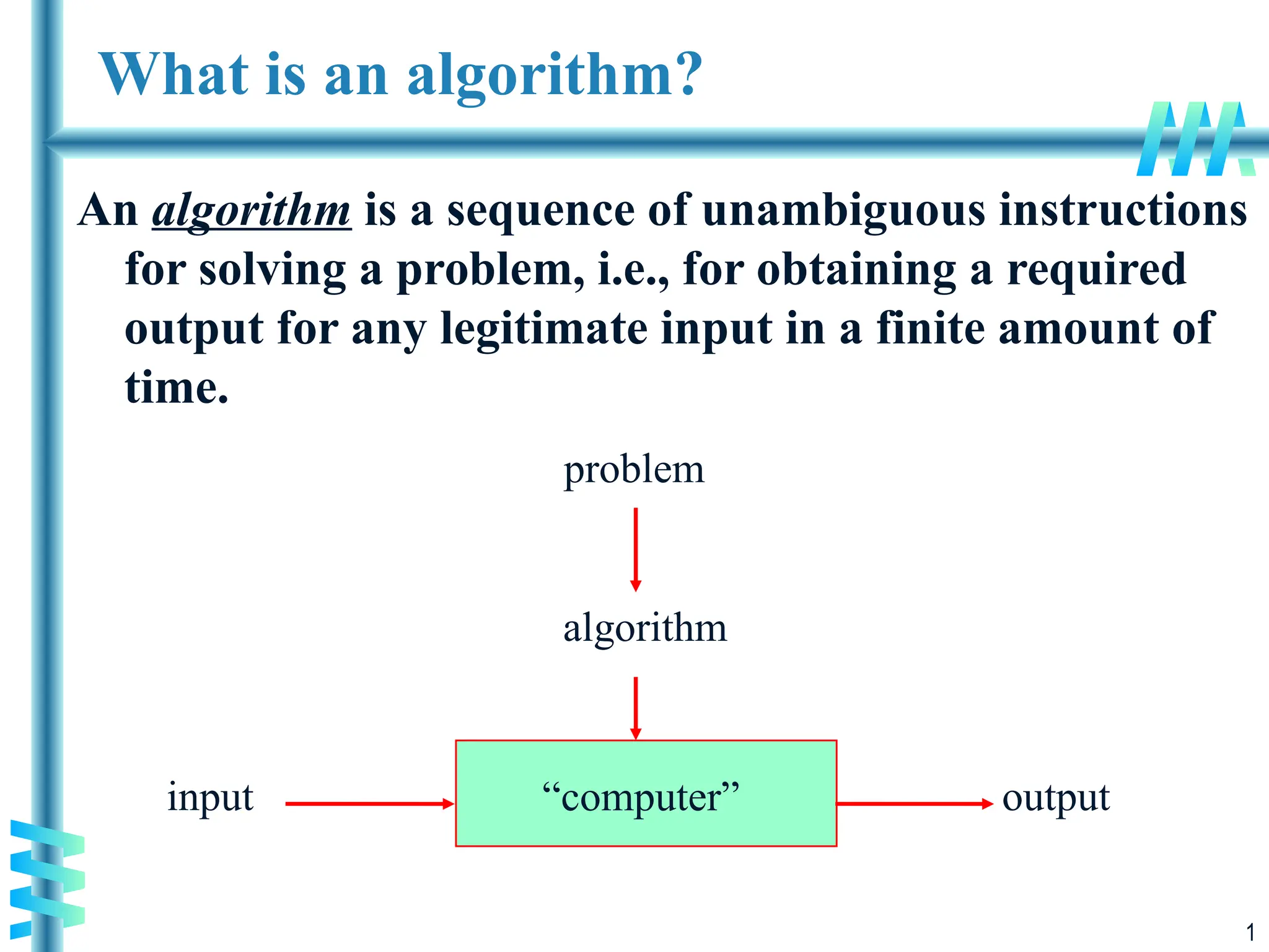
An algorithm is a sequence of unambiguous instructions
for solving a problem, i.e., for obtaining a required
output for any legitimate input in a finite amount of
time.
“computer”
problem
algorithm
input output
2.
2
What is analgorithm?
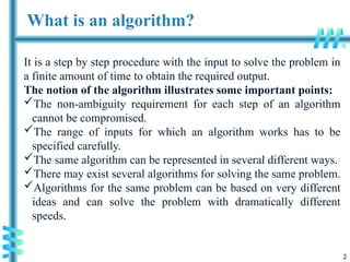
It is a step by step procedure with the input to solve the problem in
a finite amount of time to obtain the required output.
The notion of the algorithm illustrates some important points:
The non-ambiguity requirement for each step of an algorithm
cannot be compromised.
The range of inputs for which an algorithm works has to be
specified carefully.
The same algorithm can be represented in several different ways.
There may exist several algorithms for solving the same problem.
Algorithms for the same problem can be based on very different
ideas and can solve the problem with dramatically different
speeds.
9
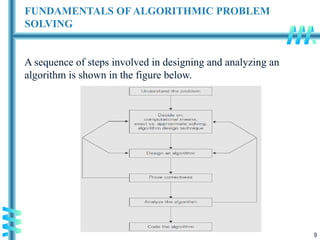
FUNDAMENTALS OF ALGORITHMICPROBLEM
SOLVING
A sequence of steps involved in designing and analyzing an
algorithm is shown in the figure below.
10.
10
Cont..
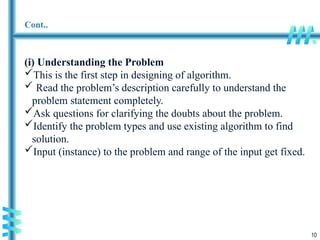
(i) Understanding theProblem
This is the first step in designing of algorithm.
Read the problem’s description carefully to understand the
problem statement completely.
Ask questions for clarifying the doubts about the problem.
Identify the problem types and use existing algorithm to find
solution.
Input (instance) to the problem and range of the input get fixed.
11.
11
Cont..
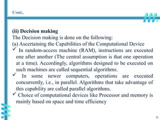
(ii) Decision making
TheDecision making is done on the following:
(a) Ascertaining the Capabilities of the Computational Device
In random-access machine (RAM), instructions are executed
one after another (The central assumption is that one operation
at a time). Accordingly, algorithms designed to be executed on
such machines are called sequential algorithms.
In some newer computers, operations are executed
concurrently, i.e., in parallel. Algorithms that take advantage of
this capability are called parallel algorithms.
Choice of computational devices like Processor and memory is
mainly based on space and time efficiency
12.
12
Cont..
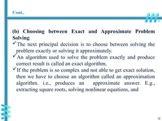
(b) Choosing betweenExact and Approximate Problem
Solving
The next principal decision is to choose between solving the
problem exactly or solving it approximately.
An algorithm used to solve the problem exactly and produce
correct result is called an exact algorithm.
If the problem is so complex and not able to get exact solution,
then we have to choose an algorithm called an approximation
algorithm. i.e., produces an approximate answer. E.g.,
extracting square roots, solving nonlinear equations, and
13.
13
Cont..
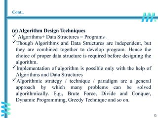
(c) Algorithm DesignTechniques
Algorithms+ Data Structures = Programs
Though Algorithms and Data Structures are independent, but
they are combined together to develop program. Hence the
choice of proper data structure is required before designing the
algorithm.
Implementation of algorithm is possible only with the help of
Algorithms and Data Structures
Algorithmic strategy / technique / paradigm are a general
approach by which many problems can be solved
algorithmically. E.g., Brute Force, Divide and Conquer,
Dynamic Programming, Greedy Technique and so on.
14.
14
Cont..
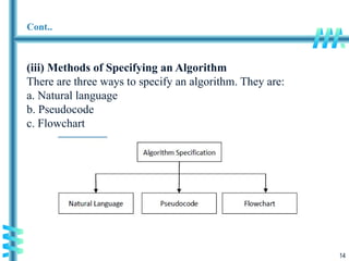
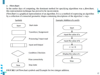
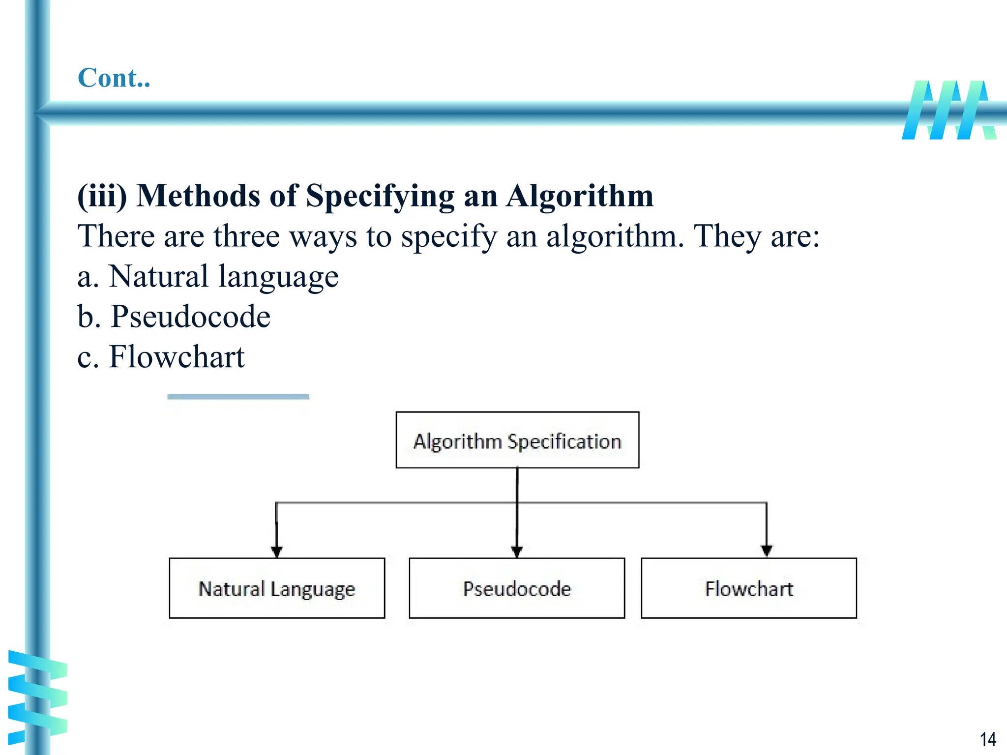
(iii) Methods ofSpecifying an Algorithm
There are three ways to specify an algorithm. They are:
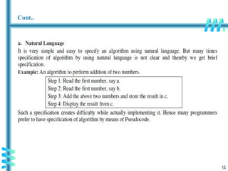
a. Natural language
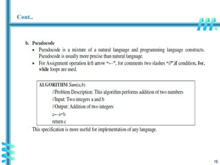
b. Pseudocode
c. Flowchart
18
Cont..
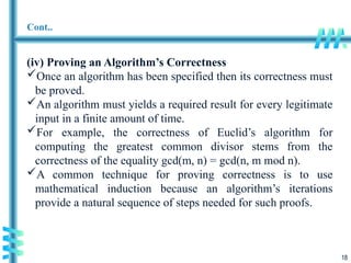
(iv) Proving anAlgorithm’s Correctness
Once an algorithm has been specified then its correctness must
be proved.
An algorithm must yields a required result for every legitimate
input in a finite amount of time.
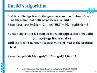
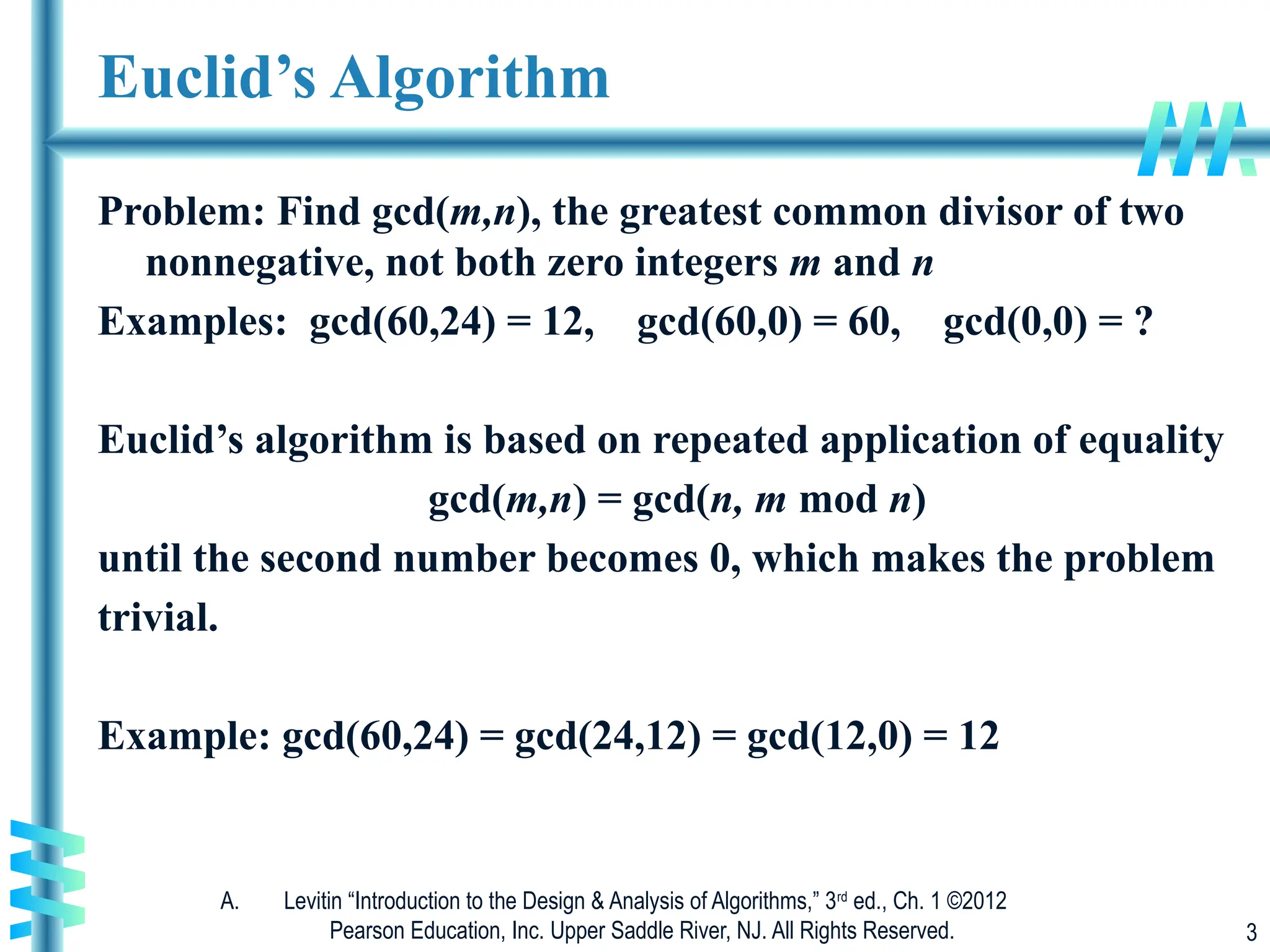
For example, the correctness of Euclid’s algorithm for
computing the greatest common divisor stems from the
correctness of the equality gcd(m, n) = gcd(n, m mod n).
A common technique for proving correctness is to use
mathematical induction because an algorithm’s iterations
provide a natural sequence of steps needed for such proofs.
20
Cont..
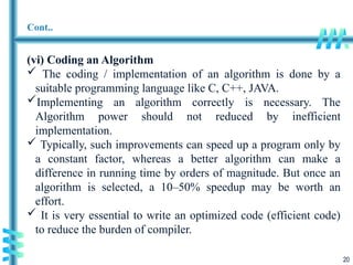
(vi) Coding anAlgorithm
The coding / implementation of an algorithm is done by a
suitable programming language like C, C++, JAVA.
Implementing an algorithm correctly is necessary. The
Algorithm power should not reduced by inefficient
implementation.
Typically, such improvements can speed up a program only by
a constant factor, whereas a better algorithm can make a
difference in running time by orders of magnitude. But once an
algorithm is selected, a 10–50% speedup may be worth an
effort.
It is very essential to write an optimized code (efficient code)
to reduce the burden of compiler.
21.
21
FUNDAMENTALS OF THEANALYSIS OF ALGORITHM
EFFICIENCY
The efficiency of an algorithm can be in terms of time and space.
The algorithm efficiency can be analyzed by the following ways.
a. Analysis Framework.
b. Asymptotic Notations and its properties.
c. Mathematical analysis for Recursive algorithms.
d. Mathematical analysis for Non-recursive algorithms.
22.
22
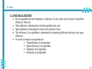
Analysis Framework
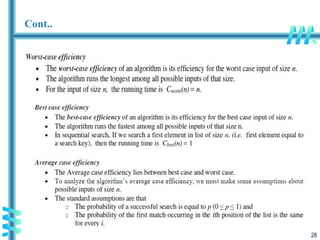
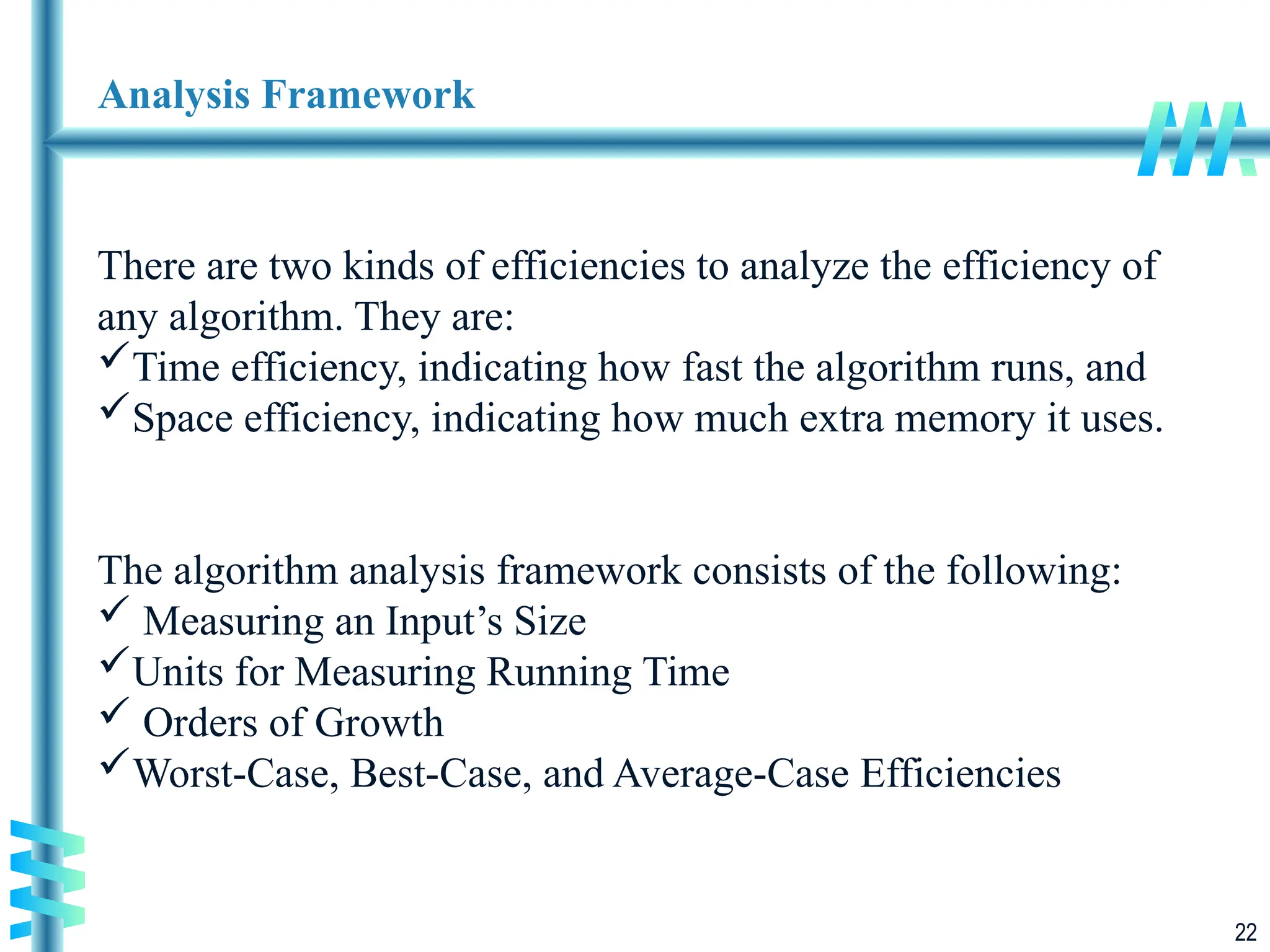
There aretwo kinds of efficiencies to analyze the efficiency of
any algorithm. They are:
Time efficiency, indicating how fast the algorithm runs, and
Space efficiency, indicating how much extra memory it uses.
The algorithm analysis framework consists of the following:
Measuring an Input’s Size
Units for Measuring Running Time
Orders of Growth
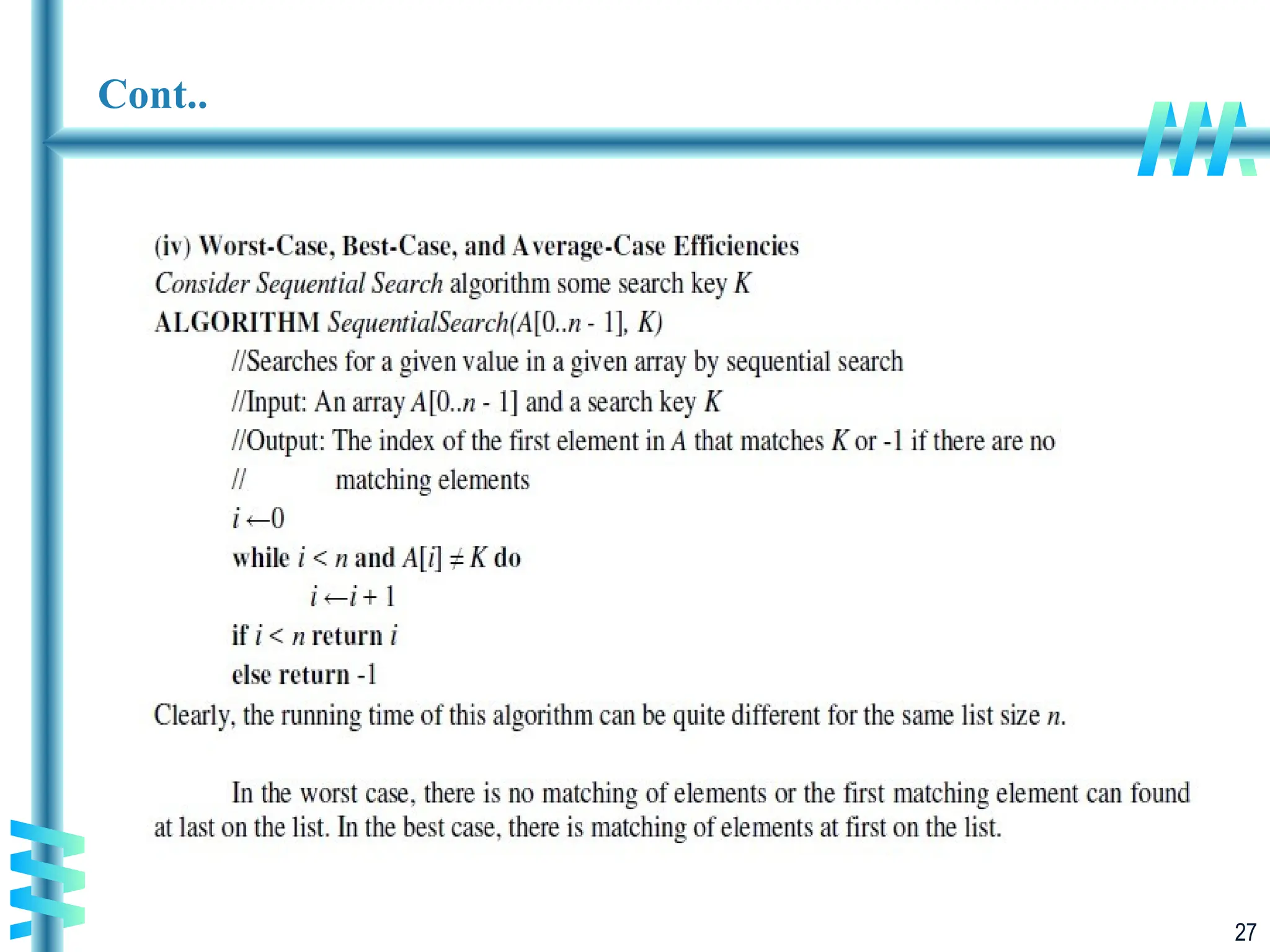
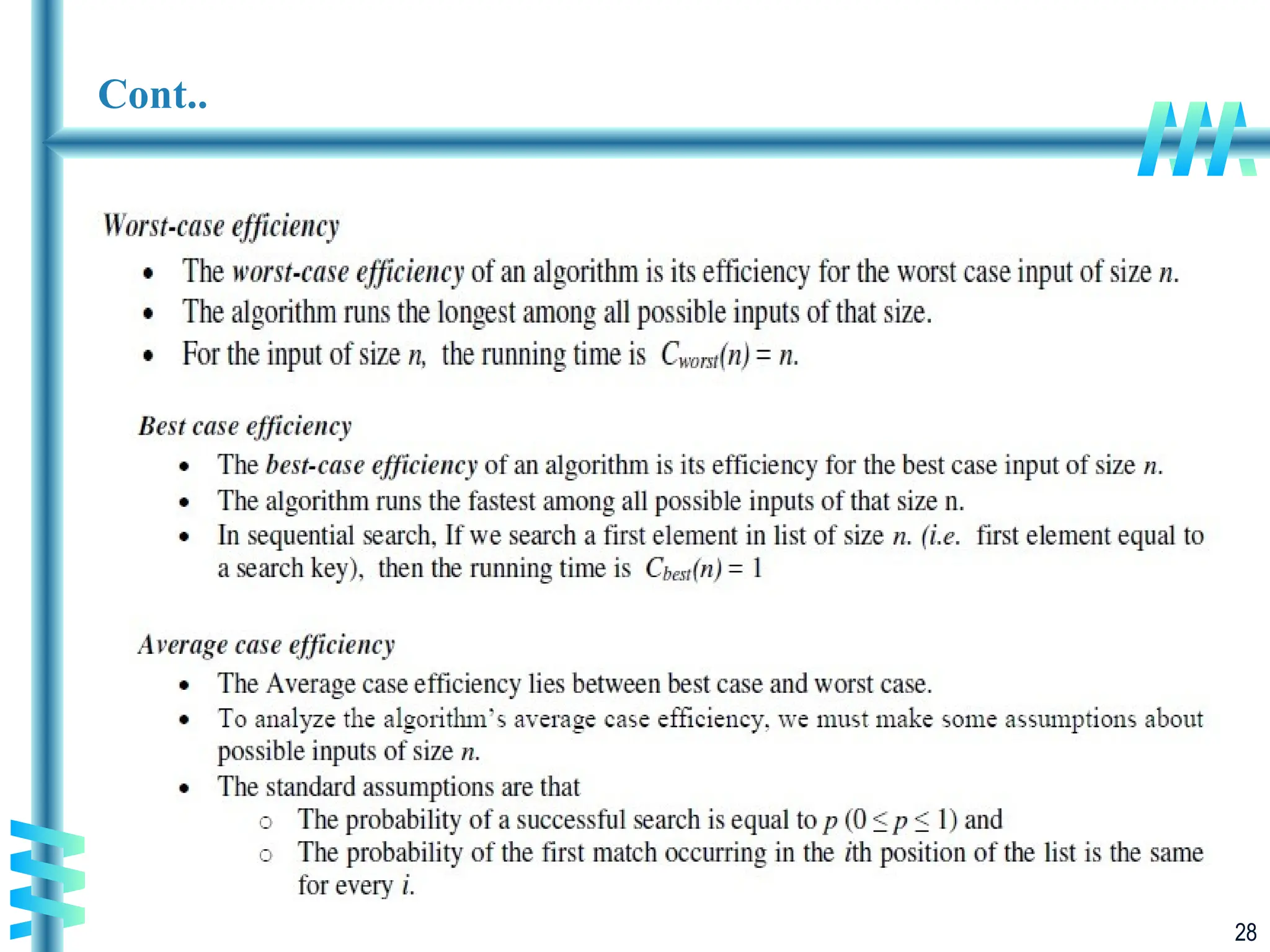
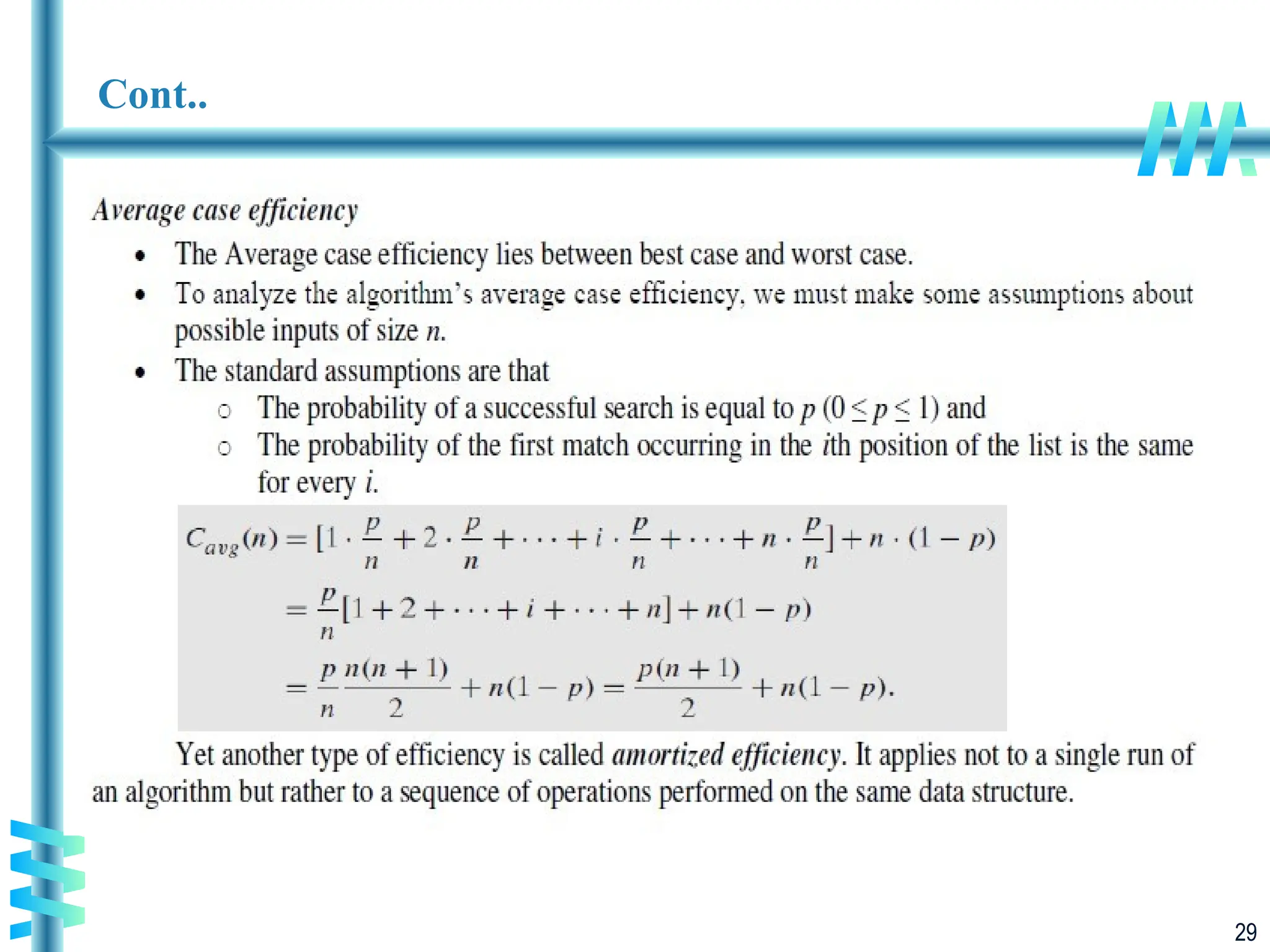
Worst-Case, Best-Case, and Average-Case Efficiencies
23.
23
Analysis Framework
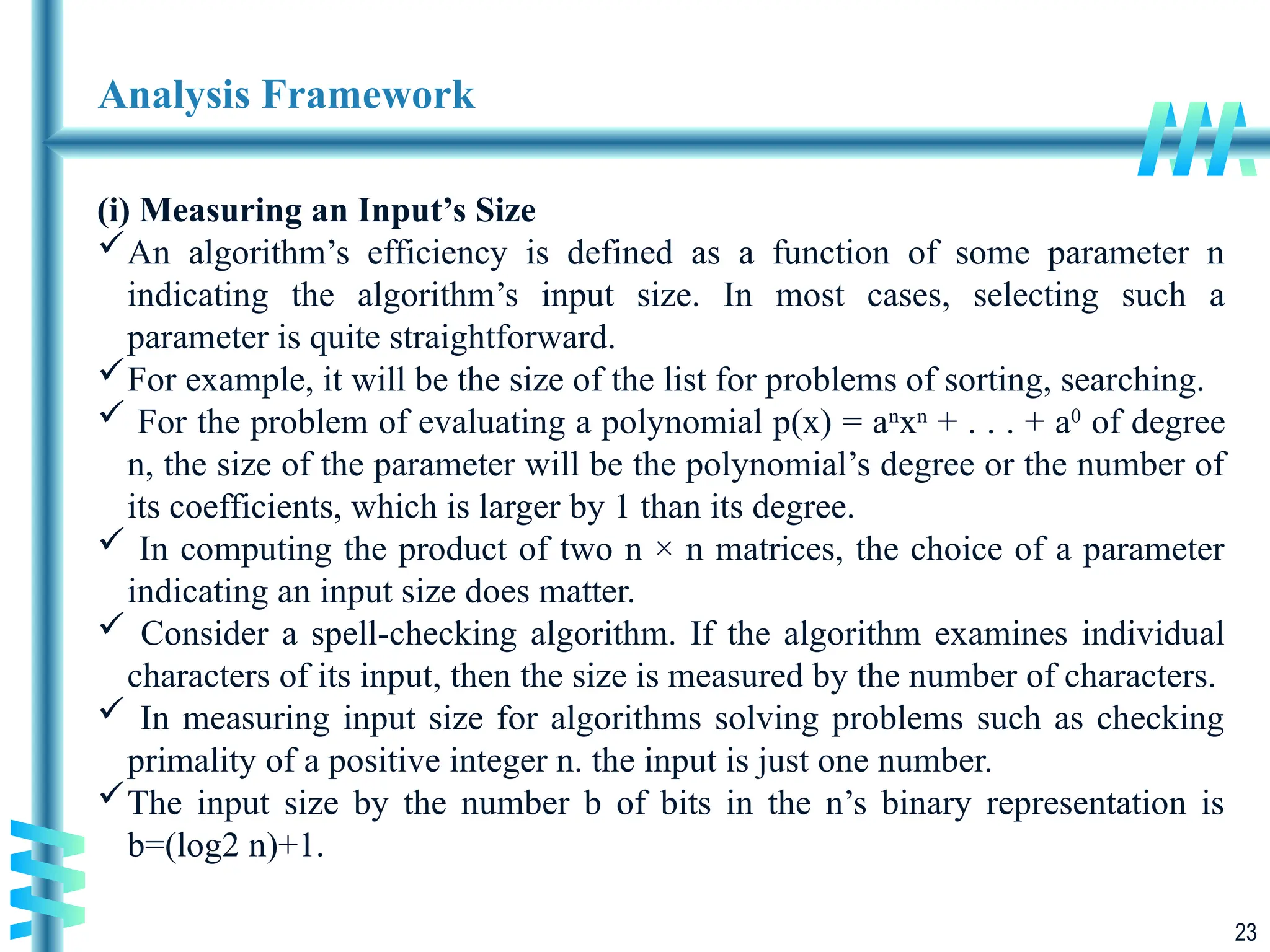
(i) Measuringan Input’s Size
An algorithm’s efficiency is defined as a function of some parameter n
indicating the algorithm’s input size. In most cases, selecting such a
parameter is quite straightforward.
For example, it will be the size of the list for problems of sorting, searching.
For the problem of evaluating a polynomial p(x) = an
xn
+ . . . + a0
of degree
n, the size of the parameter will be the polynomial’s degree or the number of
its coefficients, which is larger by 1 than its degree.
In computing the product of two n × n matrices, the choice of a parameter
indicating an input size does matter.
Consider a spell-checking algorithm. If the algorithm examines individual
characters of its input, then the size is measured by the number of characters.
In measuring input size for algorithms solving problems such as checking
primality of a positive integer n. the input is just one number.
The input size by the number b of bits in the n’s binary representation is
b=(log2 n)+1.
24.
24
Analysis Framework
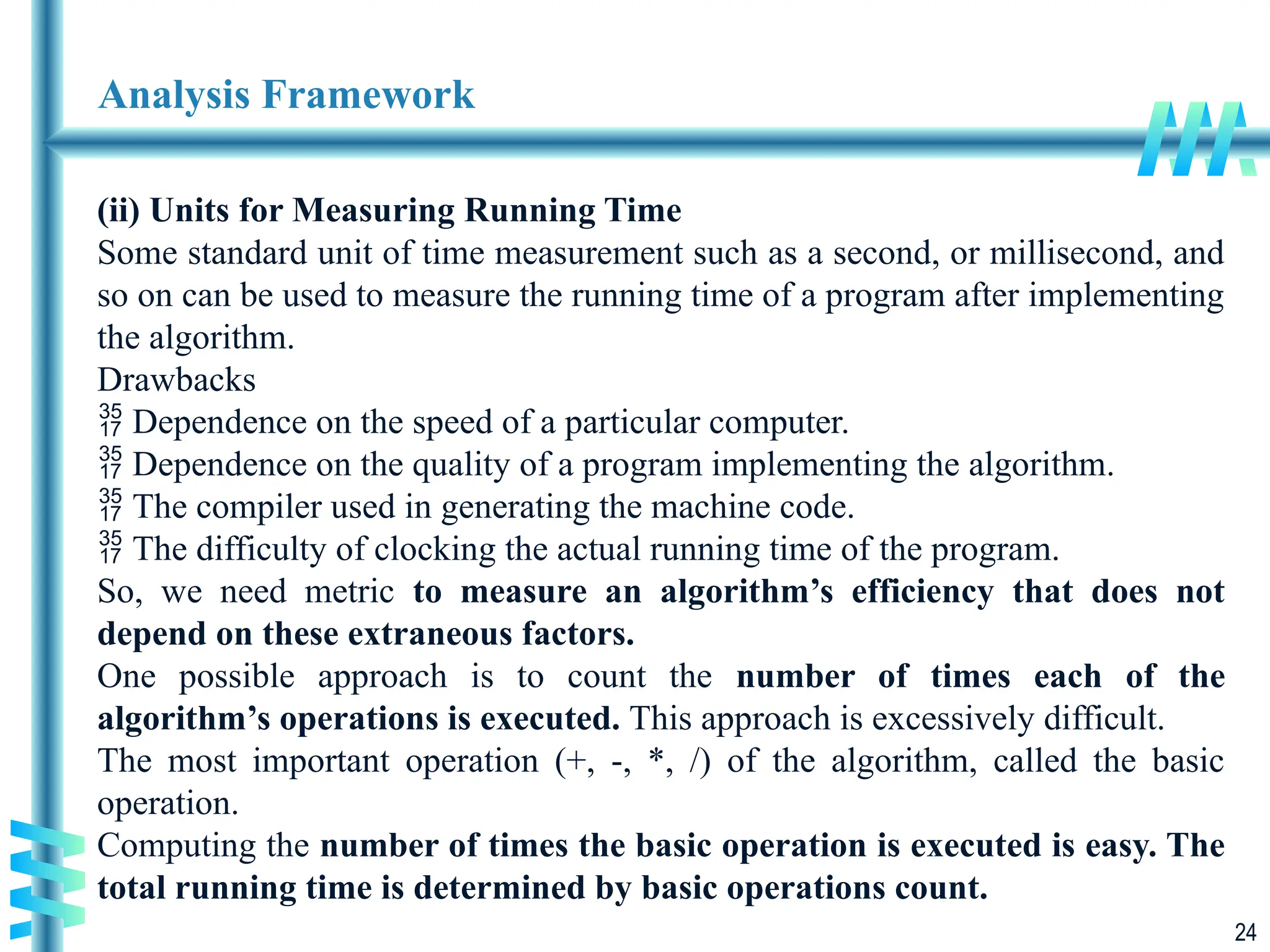
(ii) Unitsfor Measuring Running Time
Some standard unit of time measurement such as a second, or millisecond, and
so on can be used to measure the running time of a program after implementing
the algorithm.
Drawbacks
Dependence on the speed of a particular computer.
Dependence on the quality of a program implementing the algorithm.
The compiler used in generating the machine code.
The difficulty of clocking the actual running time of the program.
So, we need metric to measure an algorithm’s efficiency that does not
depend on these extraneous factors.
One possible approach is to count the number of times each of the
algorithm’s operations is executed. This approach is excessively difficult.
The most important operation (+, -, *, /) of the algorithm, called the basic
operation.
Computing the number of times the basic operation is executed is easy. The
total running time is determined by basic operations count.
25.
25
Analysis Framework
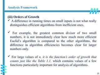
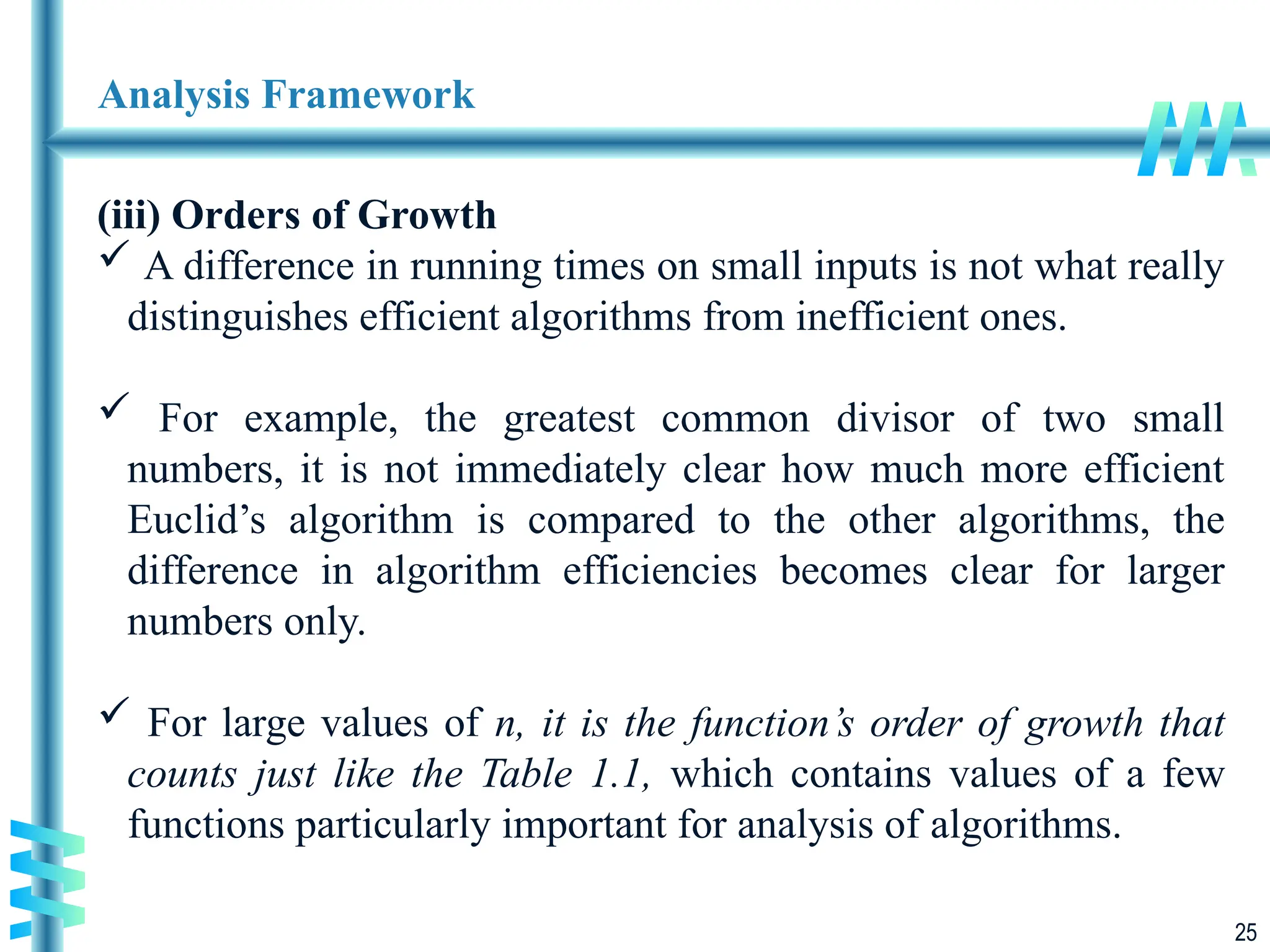
(iii) Ordersof Growth
A difference in running times on small inputs is not what really
distinguishes efficient algorithms from inefficient ones.
For example, the greatest common divisor of two small
numbers, it is not immediately clear how much more efficient
Euclid’s algorithm is compared to the other algorithms, the
difference in algorithm efficiencies becomes clear for larger
numbers only.
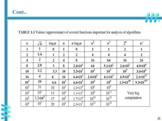
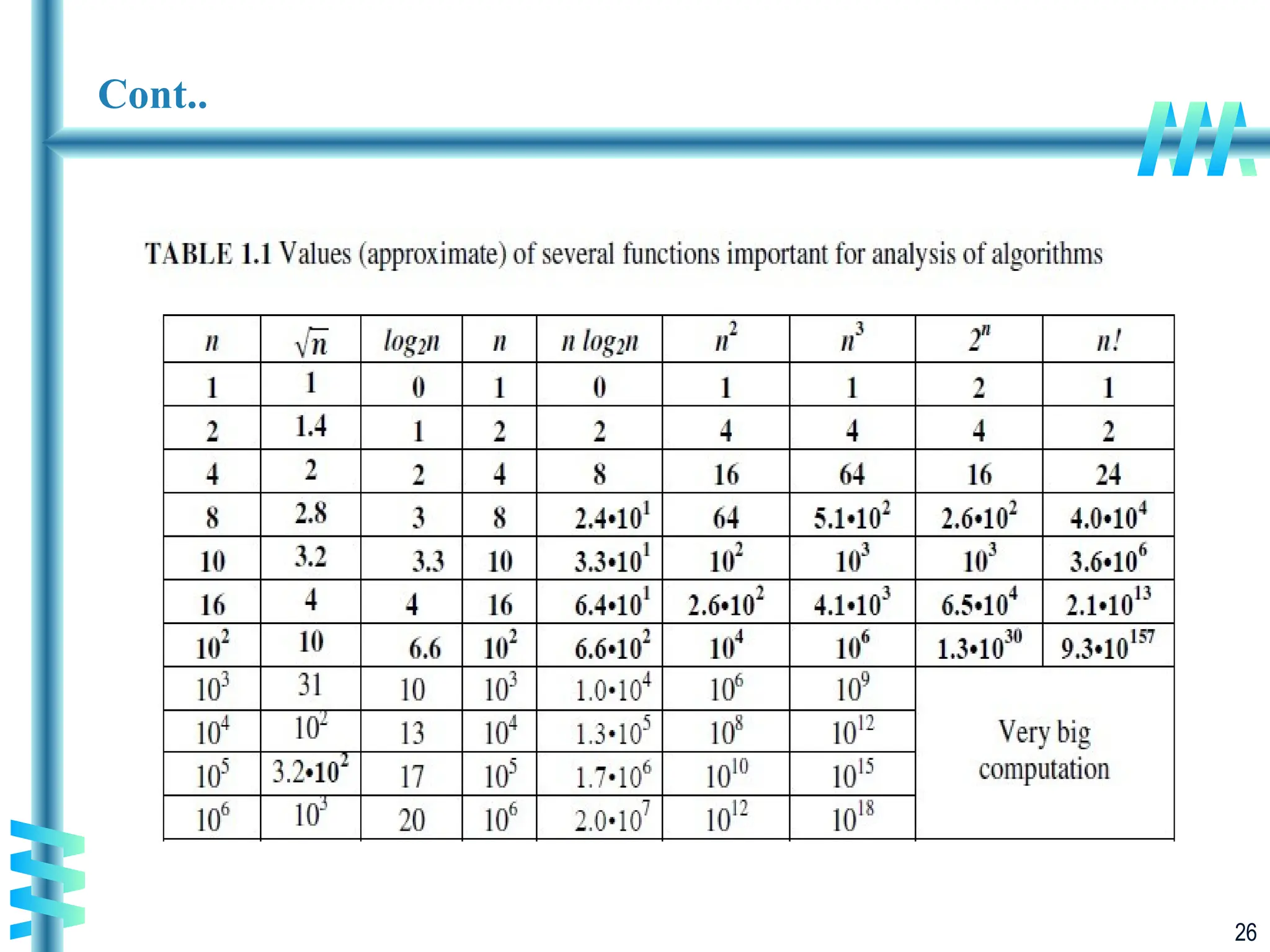
For large values of n, it is the function’s order of growth that
counts just like the Table 1.1, which contains values of a few
functions particularly important for analysis of algorithms.
30
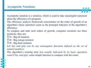
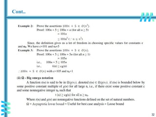
Asymptotic Notations
Asymptotic notationis a notation, which is used to take meaningful statement
about the efficiency of a program.
The efficiency analysis framework concentrates on the order of growth of an
algorithm’s basic operation count as the principal indicator of the algorithm’s
efficiency.
To compare and rank such orders of growth, computer scientists use three
notations, they are:
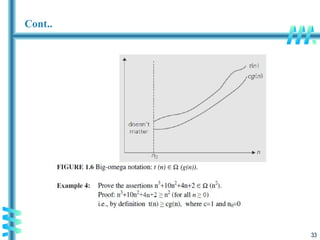
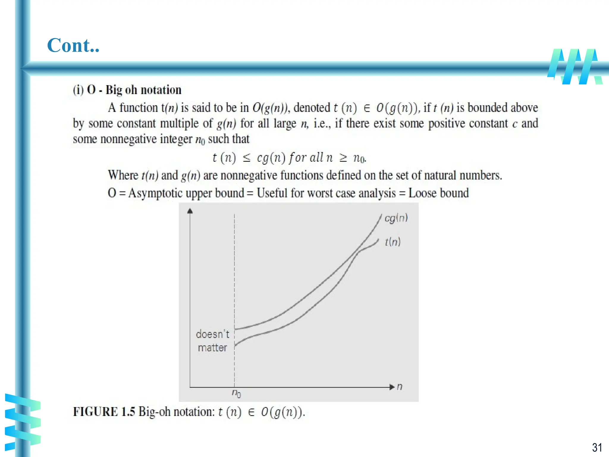
O - Big oh notation
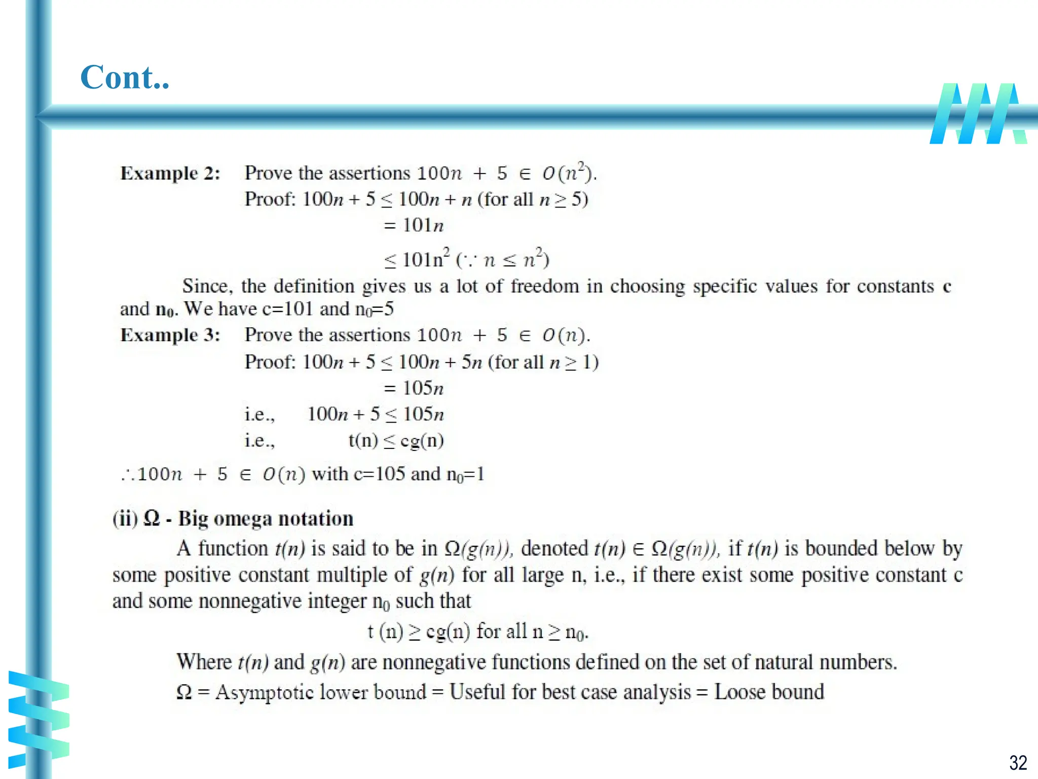
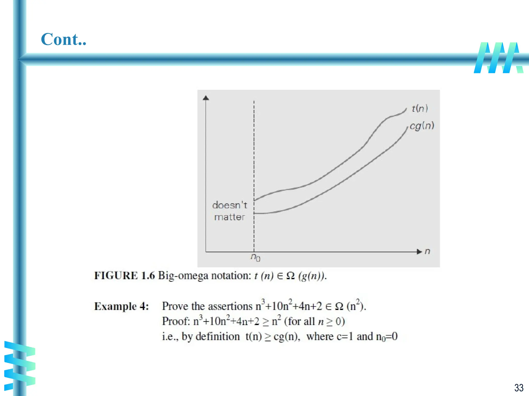
Ω - Big omega notation
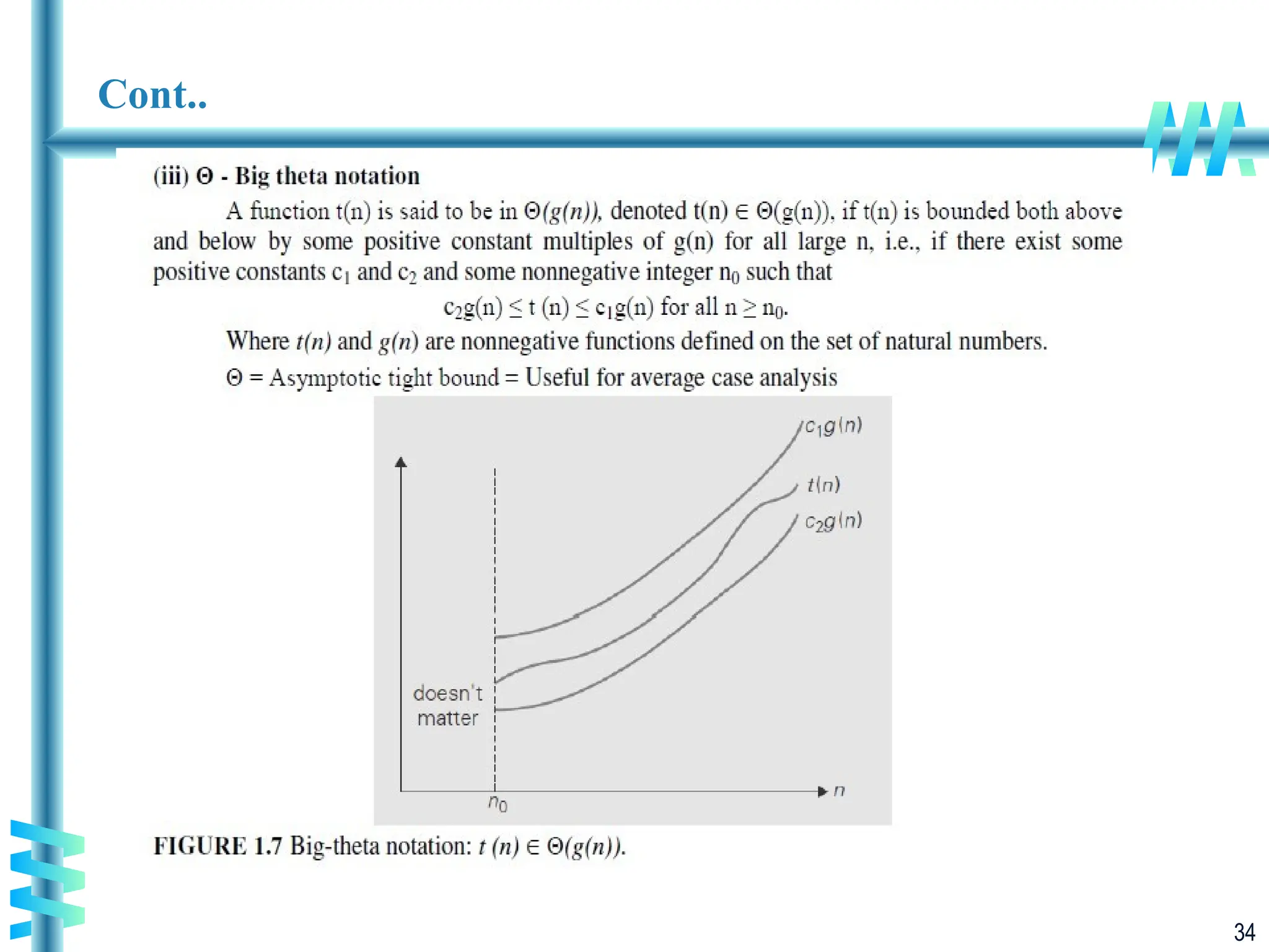
Θ - Big theta notation
Let t(n) and g(n) can be any nonnegative functions defined on the set of
natural numbers.
The algorithm’s running time t(n) usually indicated by its basic operation
count C(n), and g(n), some simple function to compare with the count.
37
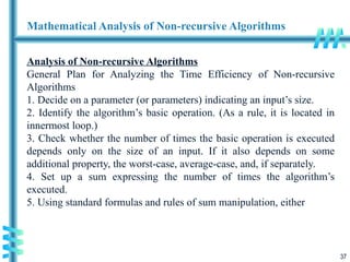
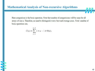
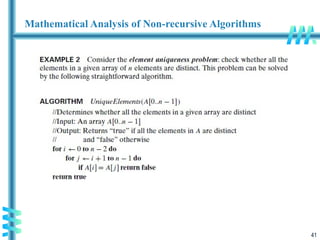
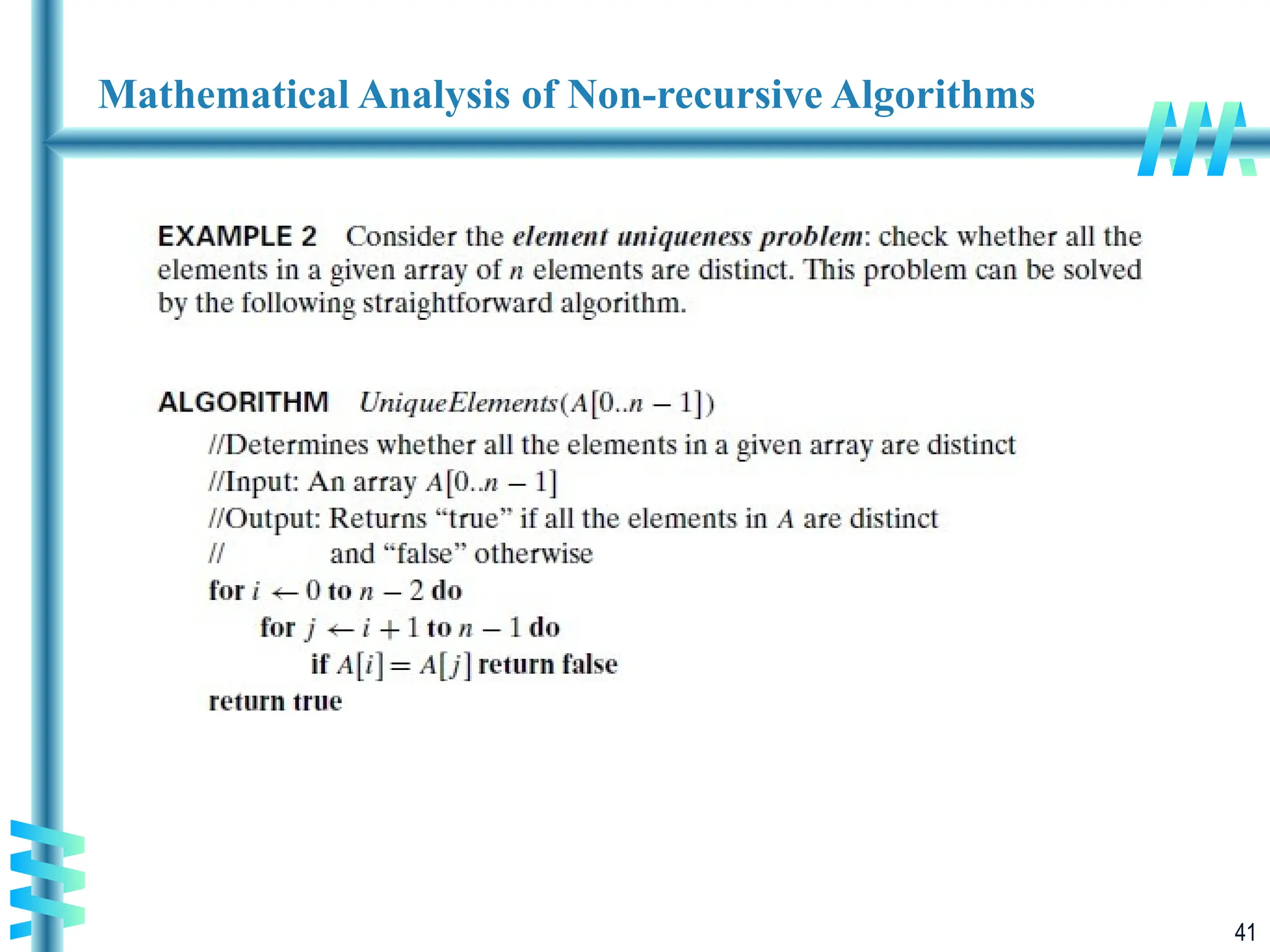
Mathematical Analysis ofNon-recursive Algorithms
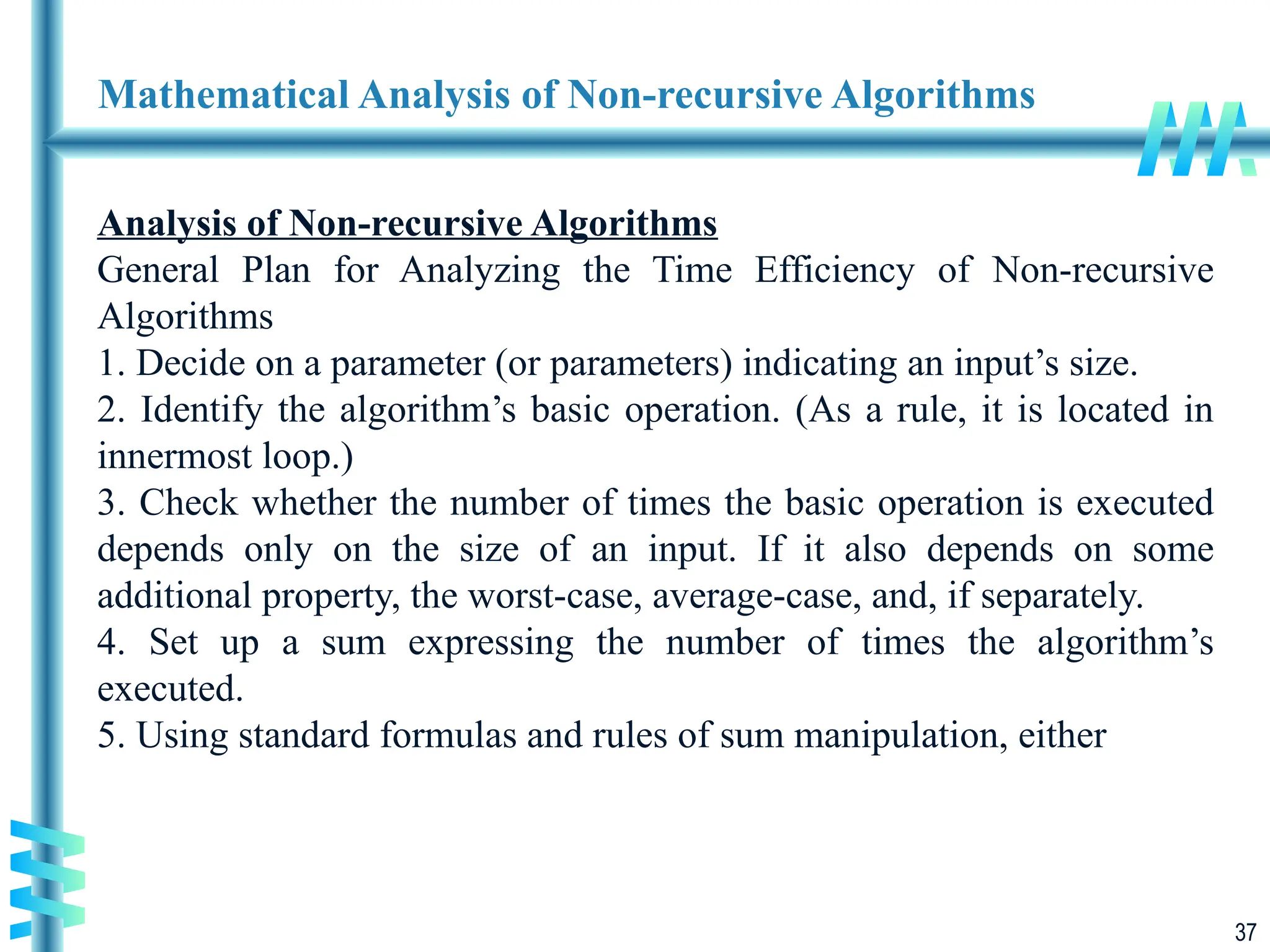
Analysis of Non-recursive Algorithms
General Plan for Analyzing the Time Efficiency of Non-recursive
Algorithms
1. Decide on a parameter (or parameters) indicating an input’s size.
2. Identify the algorithm’s basic operation. (As a rule, it is located in
innermost loop.)
3. Check whether the number of times the basic operation is executed
depends only on the size of an input. If it also depends on some
additional property, the worst-case, average-case, and, if separately.
4. Set up a sum expressing the number of times the algorithm’s
executed.
5. Using standard formulas and rules of sum manipulation, either
38.
38
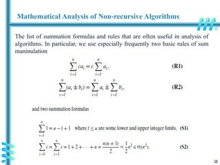
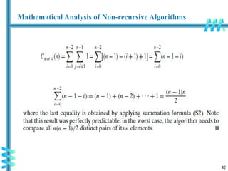
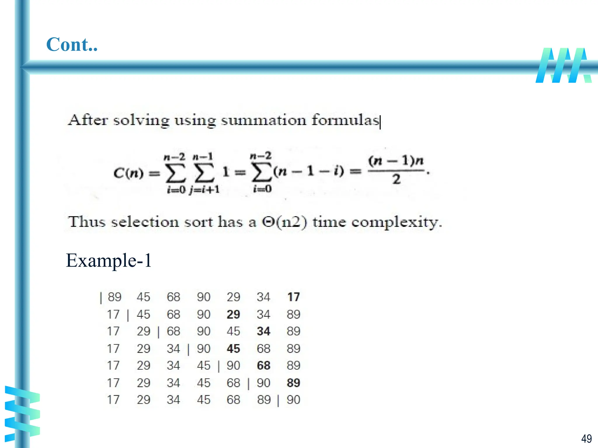
Mathematical Analysis ofNon-recursive Algorithms
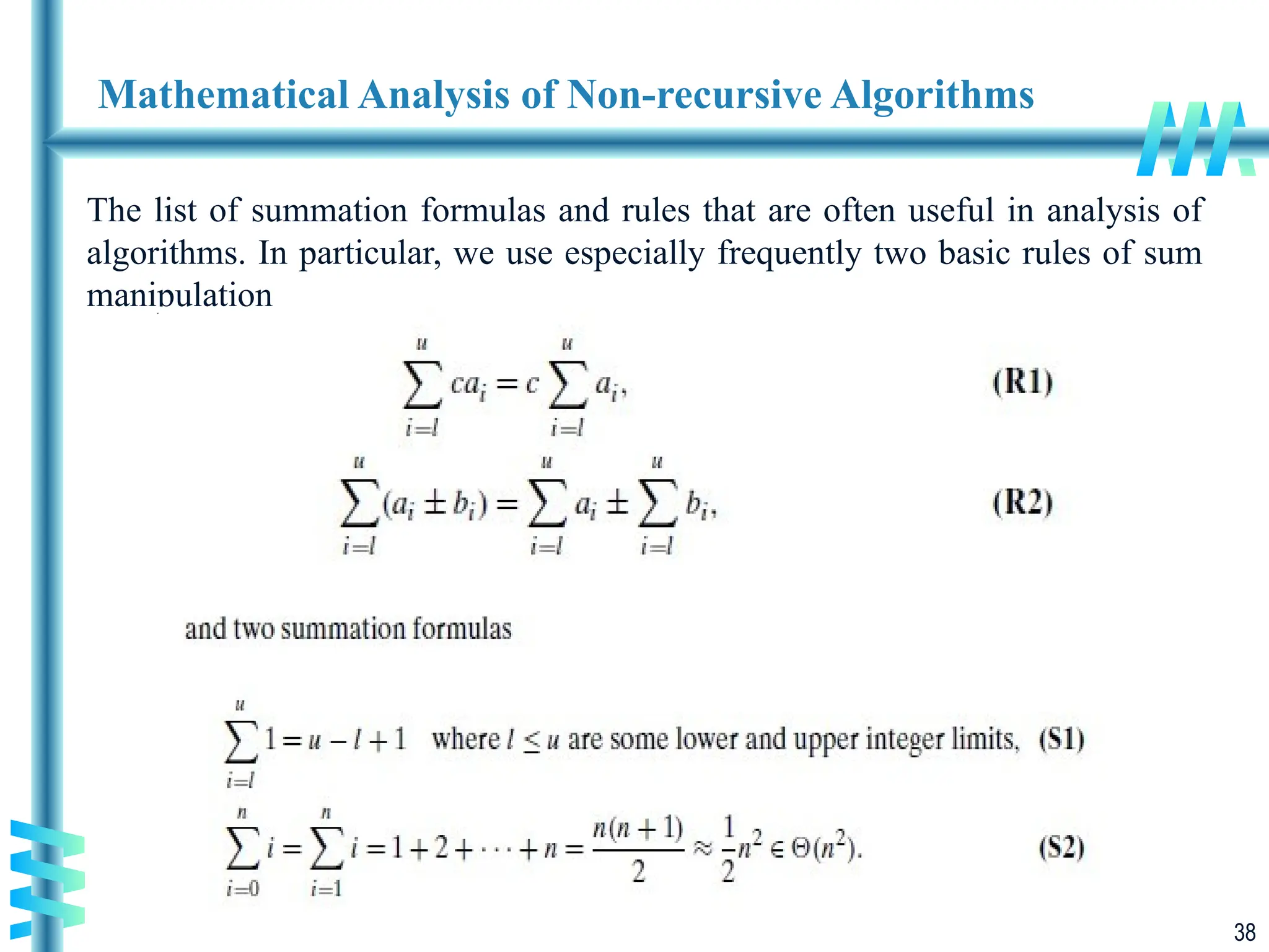
The list of summation formulas and rules that are often useful in analysis of
algorithms. In particular, we use especially frequently two basic rules of sum
manipulation
43
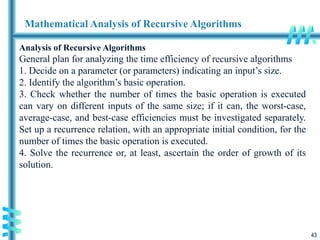
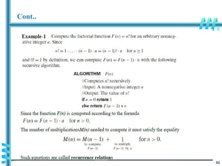
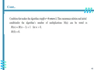
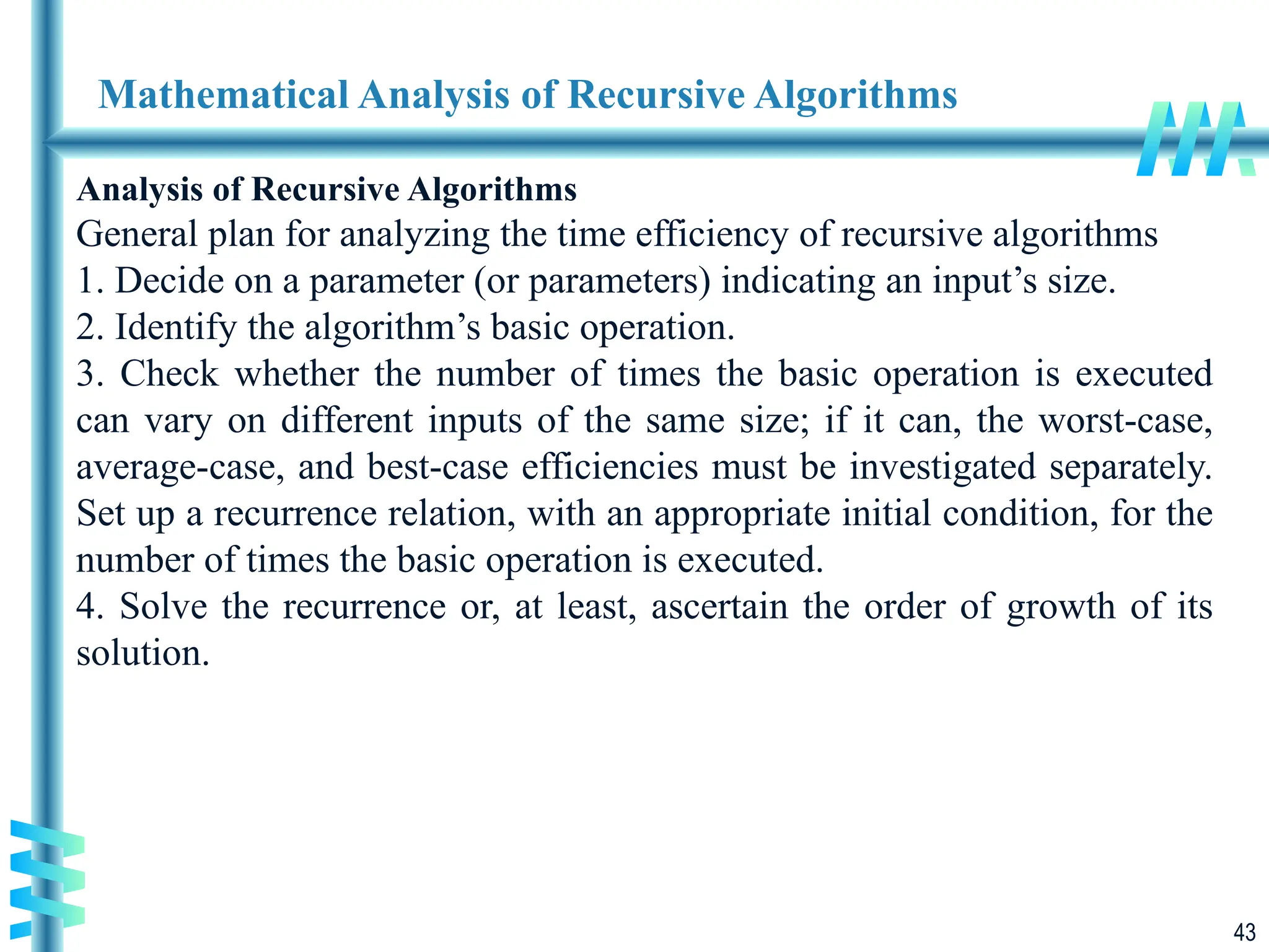
Mathematical Analysis ofRecursive Algorithms
Analysis of Recursive Algorithms
General plan for analyzing the time efficiency of recursive algorithms
1. Decide on a parameter (or parameters) indicating an input’s size.
2. Identify the algorithm’s basic operation.
3. Check whether the number of times the basic operation is executed
can vary on different inputs of the same size; if it can, the worst-case,
average-case, and best-case efficiencies must be investigated separately.
Set up a recurrence relation, with an appropriate initial condition, for the
number of times the basic operation is executed.
4. Solve the recurrence or, at least, ascertain the order of growth of its
solution.
46
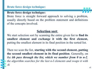
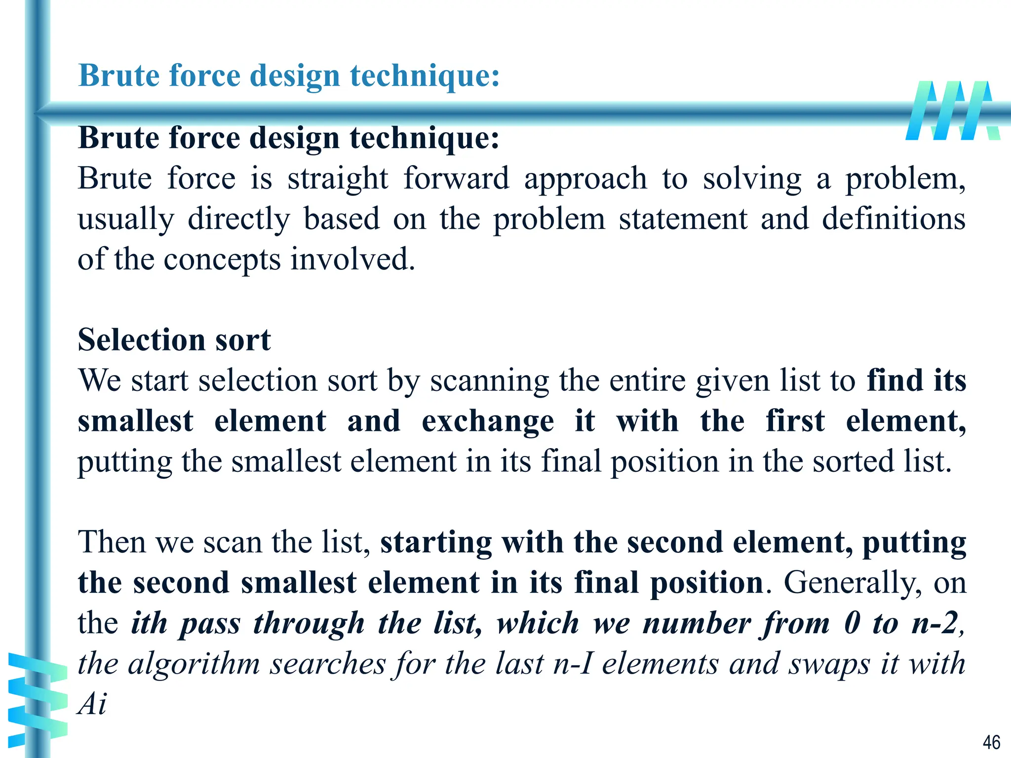
Brute force designtechnique:
Brute force design technique:
Brute force is straight forward approach to solving a problem,
usually directly based on the problem statement and definitions
of the concepts involved.
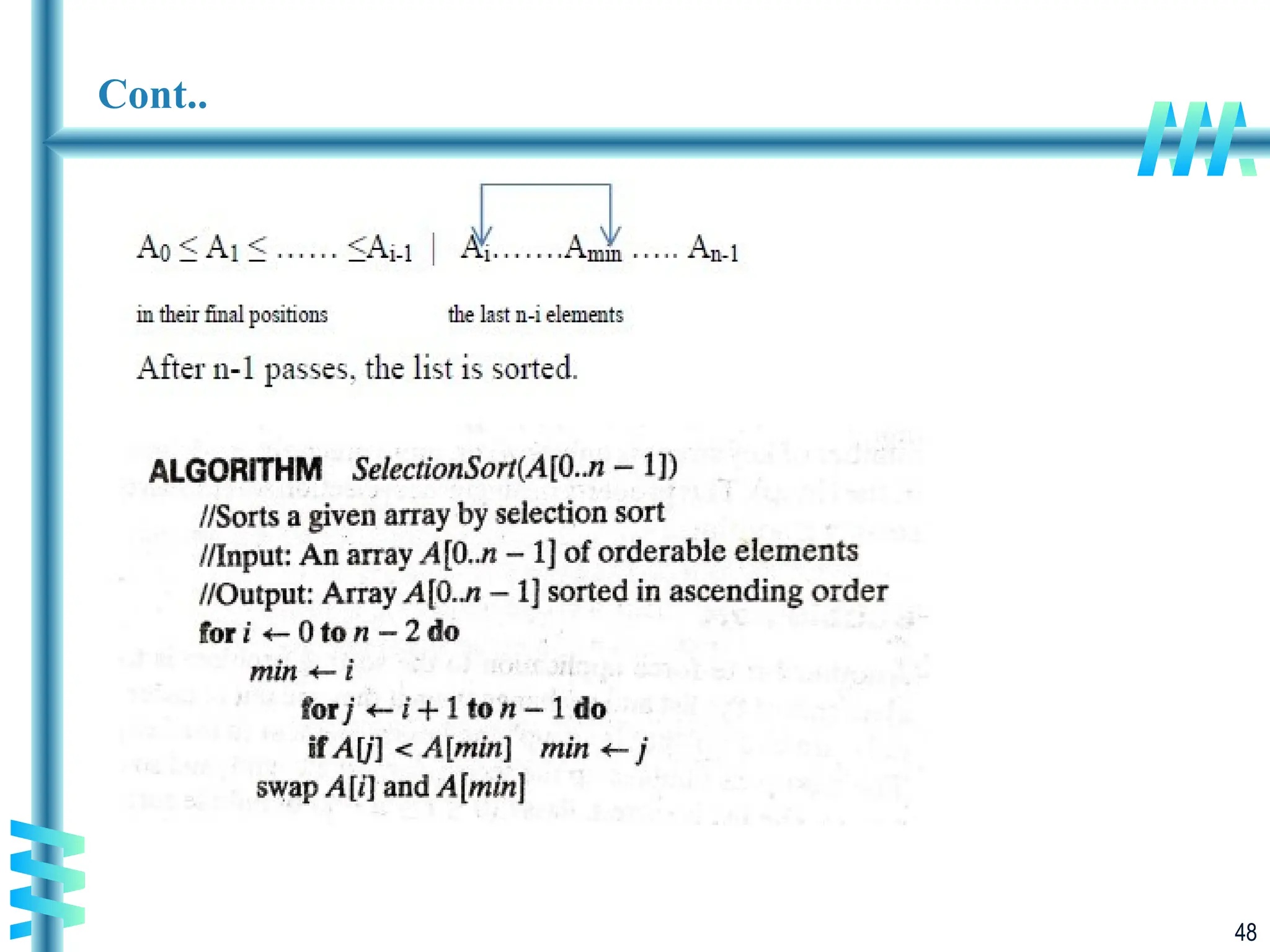
Selection sort
We start selection sort by scanning the entire given list to find its
smallest element and exchange it with the first element,
putting the smallest element in its final position in the sorted list.
Then we scan the list, starting with the second element, putting
the second smallest element in its final position. Generally, on
the ith pass through the list, which we number from 0 to n-2,
the algorithm searches for the last n-I elements and swaps it with
Ai
47.
47
Brute force designtechnique:
Brute force design technique:
Brute force is straight forward approach to solving a problem,
usually directly based on the problem statement and definitions
of the concepts involved.
Selection sort
We start selection sort by scanning the entire given list to find its
smallest element and exchange it with the first element,
putting the smallest element in its final position in the sorted list.
Then we scan the list, starting with the second element, putting
the second smallest element in its final position. Generally, on
the ith pass through the list, which we number from 0 to n-2,
the algorithm searches for the last n-I elements and swaps it with
Ai
50
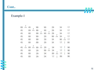
Cont..
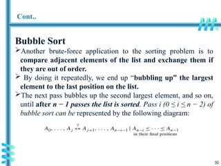
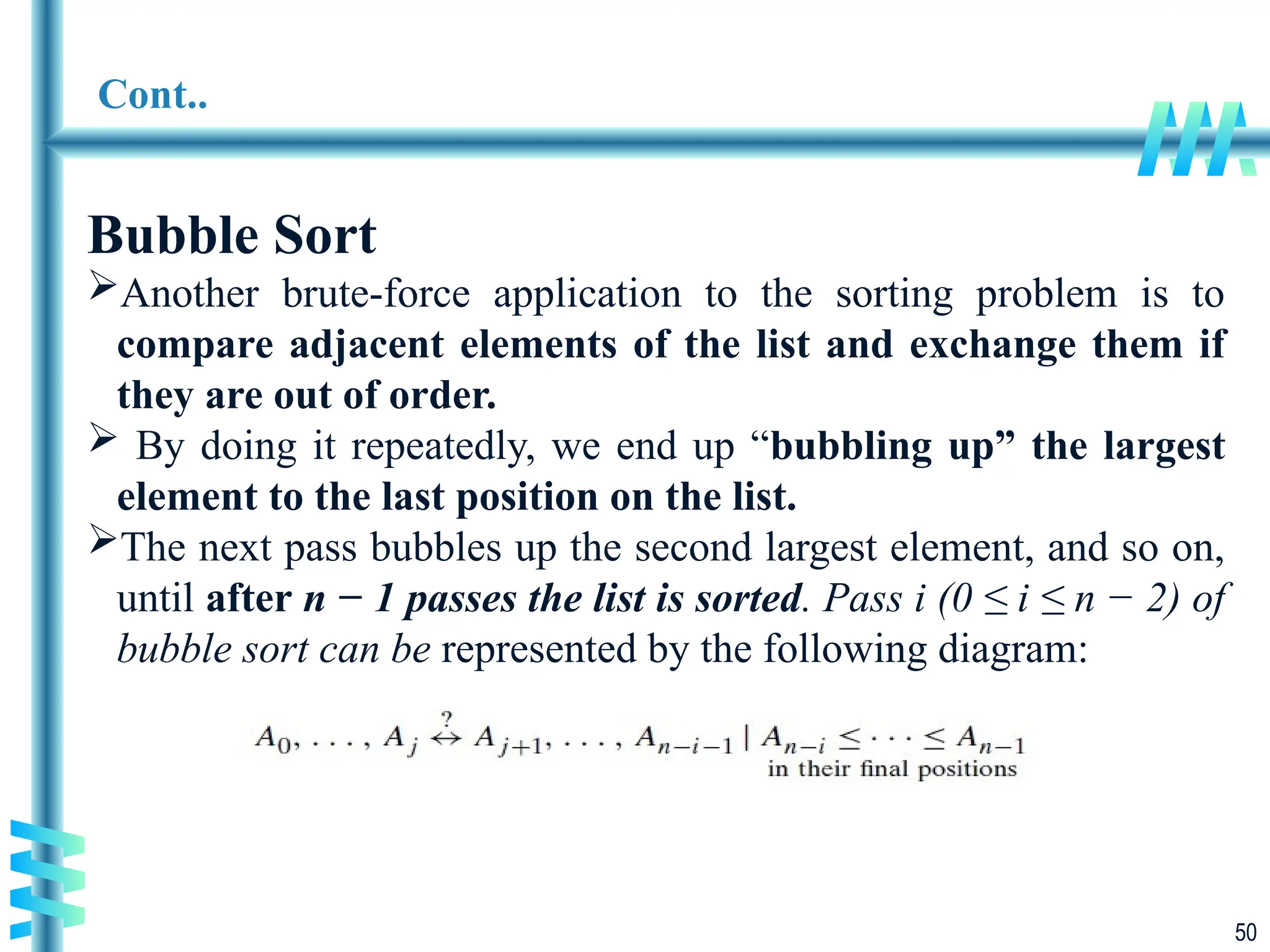
Bubble Sort
Another brute-forceapplication to the sorting problem is to
compare adjacent elements of the list and exchange them if
they are out of order.
By doing it repeatedly, we end up “bubbling up” the largest
element to the last position on the list.
The next pass bubbles up the second largest element, and so on,
until after n − 1 passes the list is sorted. Pass i (0 ≤ i ≤ n − 2) of
bubble sort can be represented by the following diagram:
51.
51
Cont..
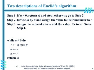
Here is pseudocodeof this algorithm.
ALGORITHM BubbleSort(A[0..n − 1])
//Sorts a given array by bubble sort
//Input: An array A[0..n − 1] of orderable elements
//Output: Array A[0..n − 1] sorted in non decreasing order
for i ←0 to n − 2 do
for j ←0 to n − 2 − i do
if A[j + 1]<A[j ]
swap A[j ] and A[j + 1]
53
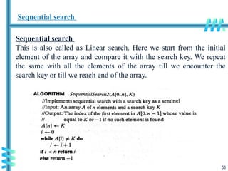
Sequential search
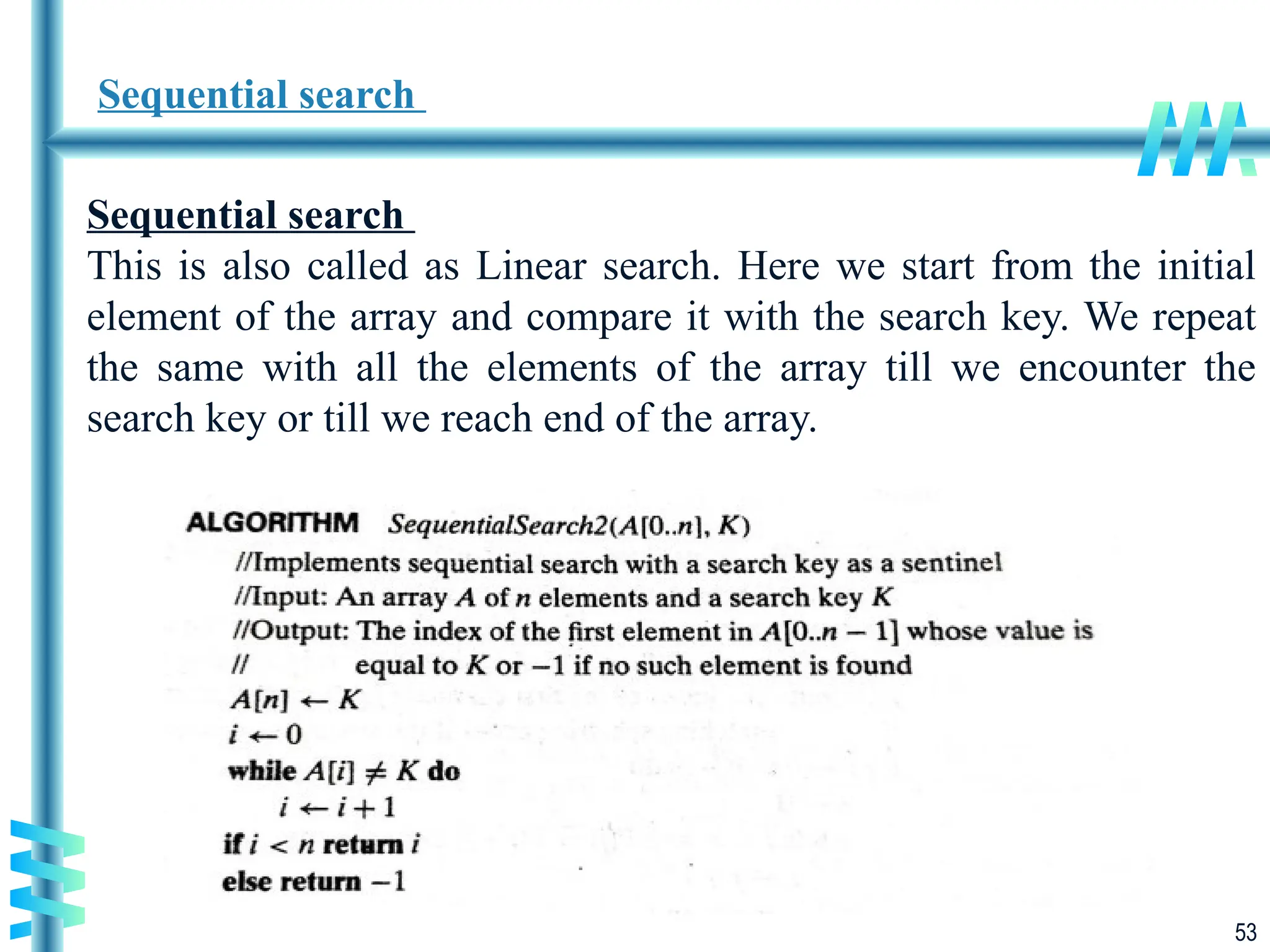
Sequential search
Thisis also called as Linear search. Here we start from the initial
element of the array and compare it with the search key. We repeat
the same with all the elements of the array till we encounter the
search key or till we reach end of the array.
54.
54
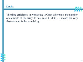
Cont..
The time efficiencyin worst case is O(n), where n is the number
of elements of the array. In best case it is O(1), it means the very
first element is the search key.
55.
55
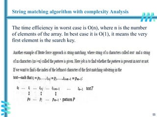
String matching algorithmwith complexity Analysis
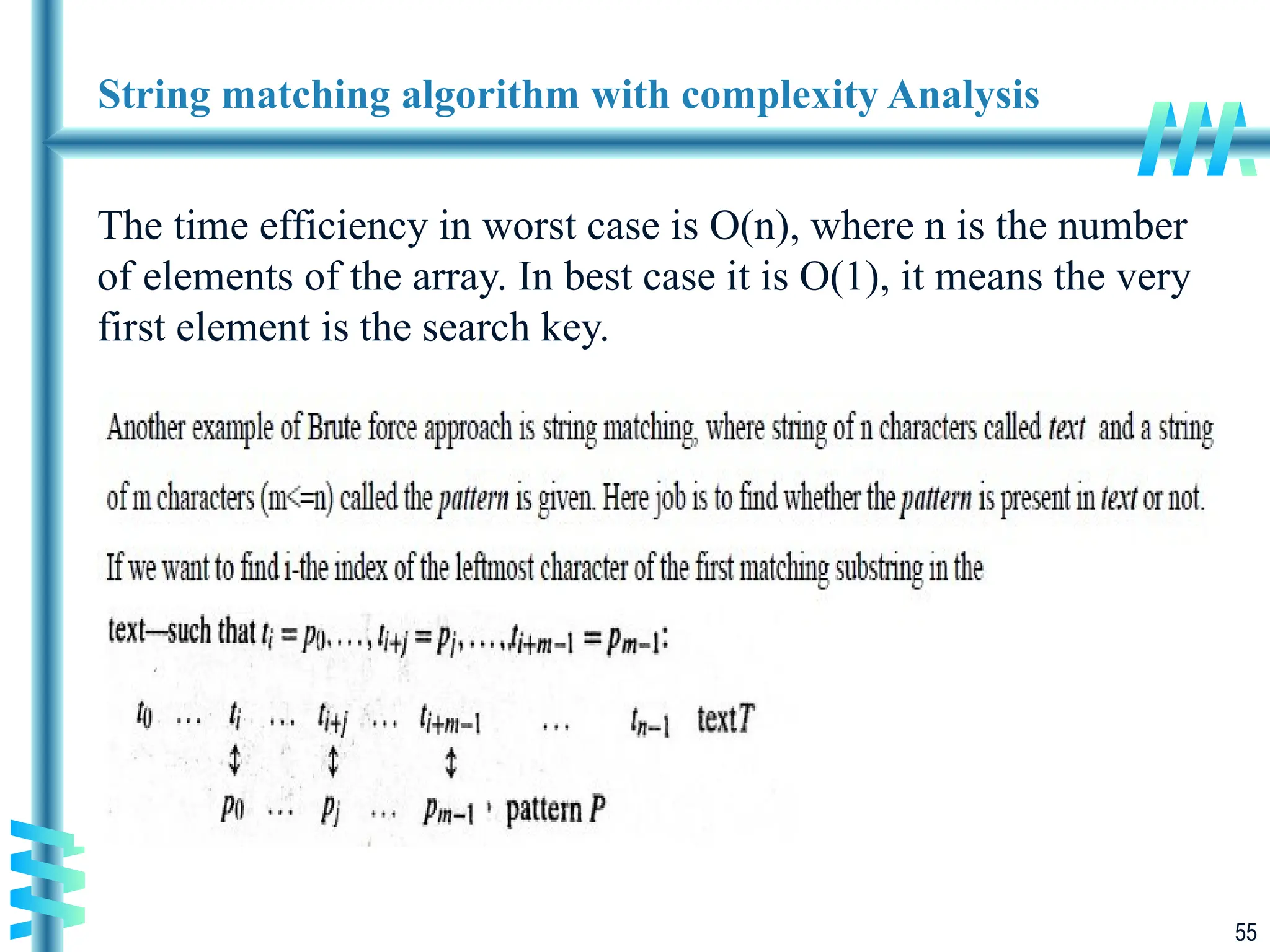
The time efficiency in worst case is O(n), where n is the number
of elements of the array. In best case it is O(1), it means the very
first element is the search key.
56.
56
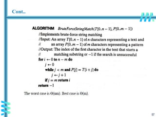
Cont..
We start matchingwith the very first character, if a match then
only j is incremented and again compared with next character
of both the strings.
If not then I is incremented and j starts from beginning of
pattern string. If pattern found we return the position from
where the pattern began.
Pattern is tried to match till n-m elements, later we need not try
to match as the elements will be lesser than pattern. If it doesn’t
match by n-m elements then pattern is not matched.
#3 Euclid’s algorithm is good for introducing the notion of an algorithm because it
makes a clear separation from a program that implements the algorithm.
It is also one that is familiar to most students.
Al Khowarizmi (many spellings possible...) – “algorism” (originally) and then
later “algorithm” come from his name.
![A. Levitin “Introduction to the Design & Analysis of Algorithms,” 3rd
ed., Ch. 1 ©2012
Pearson Education, Inc. Upper Saddle River, NJ. All Rights Reserved. 5
Other methods for gcd(m,n) [cont.]
Middle-school procedure
Step 1 Find the prime factorization of m
Step 2 Find the prime factorization of n
Step 3 Find all the common prime factors
Step 4 Compute the product of all the common prime factors
and return it as gcd(m,n)
Is this an algorithm?](https://image.slidesharecdn.com/module-1-250329084404-4b6d0f28/85/Analysis-Framework-Asymptotic-Notations-5-320.jpg)

![A. Levitin “Introduction to the Design & Analysis of Algorithms,” 3rd
ed., Ch. 1 ©2012
Pearson Education, Inc. Upper Saddle River, NJ. All Rights Reserved. 8
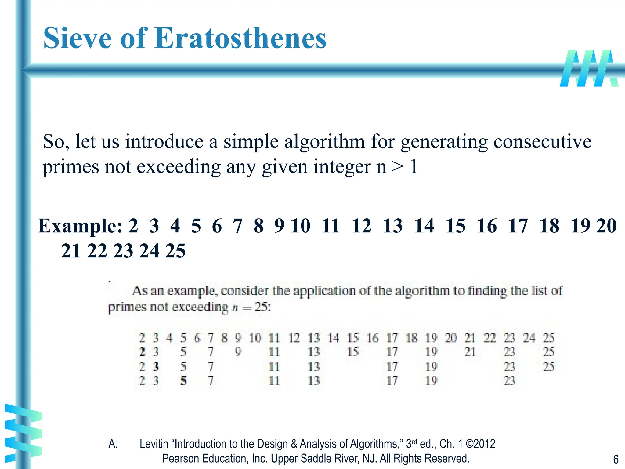
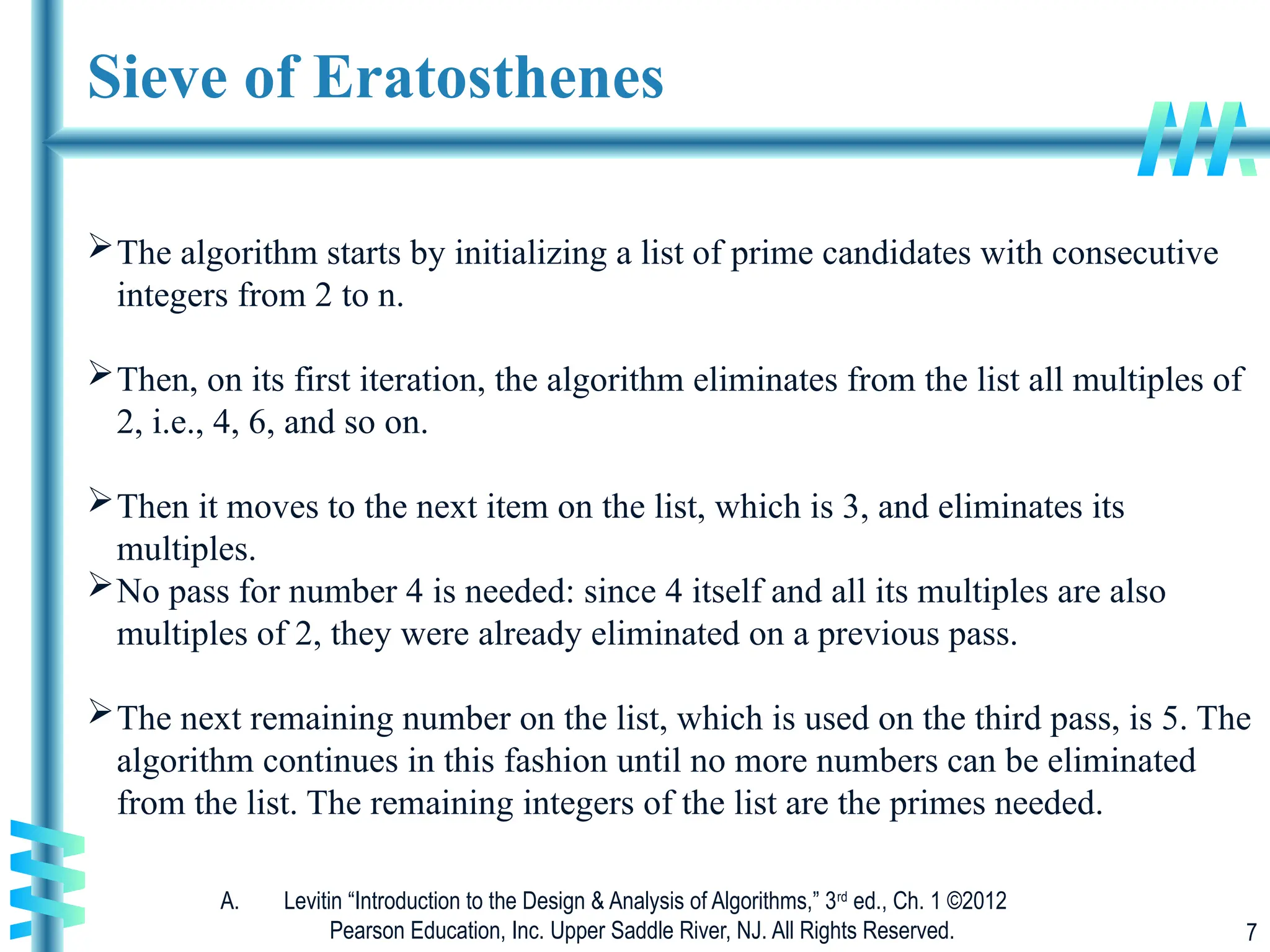
Sieve of Eratosthenes
Input: Integer n ≥ 2
Output: List of primes less than or equal to n
for p ← 2 to n do A[p] ← p
for p ← 2 to n do
if A[p] 0 //p hasn’t been previously eliminated from the list
j ← p* p
while j ≤ n do
A[j] ← 0 //mark element as eliminated
j ← j + p](https://image.slidesharecdn.com/module-1-250329084404-4b6d0f28/85/Analysis-Framework-Asymptotic-Notations-8-320.jpg)


![51
Cont..
Here is pseudocode of this algorithm.
ALGORITHM BubbleSort(A[0..n − 1])
//Sorts a given array by bubble sort
//Input: An array A[0..n − 1] of orderable elements
//Output: Array A[0..n − 1] sorted in non decreasing order
for i ←0 to n − 2 do
for j ←0 to n − 2 − i do
if A[j + 1]<A[j ]
swap A[j ] and A[j + 1]](https://image.slidesharecdn.com/module-1-250329084404-4b6d0f28/85/Analysis-Framework-Asymptotic-Notations-51-320.jpg)


![A. Levitin “Introduction to the Design & Analysis of Algorithms,” 3rd
ed., Ch. 1 ©2012
Pearson Education, Inc. Upper Saddle River, NJ. All Rights Reserved. 5
Other methods for gcd(m,n) [cont.]
Middle-school procedure
Step 1 Find the prime factorization of m
Step 2 Find the prime factorization of n
Step 3 Find all the common prime factors
Step 4 Compute the product of all the common prime factors
and return it as gcd(m,n)
Is this an algorithm?](https://image.slidesharecdn.com/module-1-250329084404-4b6d0f28/75/Analysis-Framework-Asymptotic-Notations-5-2048.jpg)
![A. Levitin “Introduction to the Design & Analysis of Algorithms,” 3rd
ed., Ch. 1 ©2012
Pearson Education, Inc. Upper Saddle River, NJ. All Rights Reserved. 8
Sieve of Eratosthenes
Input: Integer n ≥ 2
Output: List of primes less than or equal to n
for p ← 2 to n do A[p] ← p
for p ← 2 to n do
if A[p] 0 //p hasn’t been previously eliminated from the list
j ← p* p
while j ≤ n do
A[j] ← 0 //mark element as eliminated
j ← j + p](https://image.slidesharecdn.com/module-1-250329084404-4b6d0f28/75/Analysis-Framework-Asymptotic-Notations-8-2048.jpg)


![51
Cont..
Here is pseudocode of this algorithm.
ALGORITHM BubbleSort(A[0..n − 1])
//Sorts a given array by bubble sort
//Input: An array A[0..n − 1] of orderable elements
//Output: Array A[0..n − 1] sorted in non decreasing order
for i ←0 to n − 2 do
for j ←0 to n − 2 − i do
if A[j + 1]<A[j ]
swap A[j ] and A[j + 1]](https://image.slidesharecdn.com/module-1-250329084404-4b6d0f28/75/Analysis-Framework-Asymptotic-Notations-51-2048.jpg)