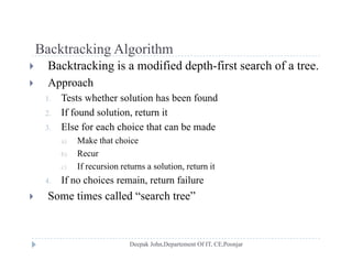
Download as PDF, PPTX
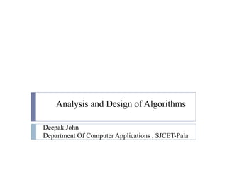
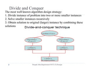
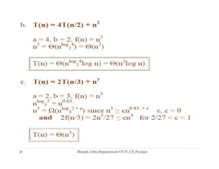
![Sequential Search, Unordered
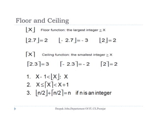
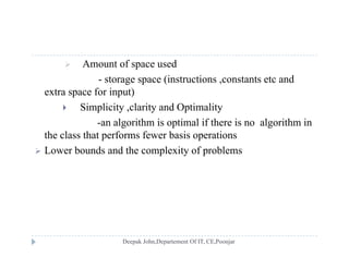
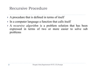
I t E K h E i ith t i i d d 0 1) dInput: E, n, K, where E is an array with n entries indexed 0, …, n-1), and
K is the item sought. For simplicity, we assume that K and the entries
of E are integers, as is n.
Output: Returns ans, the location of K in E (-1 if K is not found.)
Algorithm: Step (Specification)
int seqSearch(int[] E, int n, int K)
1. int ans, index;
2 1 // A f il2. ans = -1; // Assume failure.
3. for (index = 0; index < n; index++)
4 if (K == E[index])4. if (K E[index])
5. ans = index; // Success!
6. break; // Done!;
7. return ans;](https://image.slidesharecdn.com/anlysisanddesignofalgorithms-part1-130312001535-phpapp01/85/Anlysis-and-design-of-algorithms-part-1-12-320.jpg)
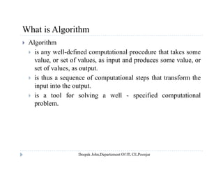
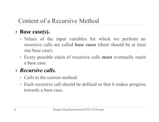
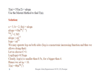
![o-notationo notation
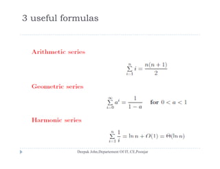
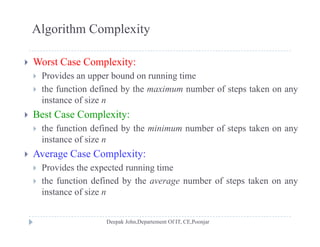
For a given function g(n), the set little-o:
f(n)=o(g(n)) there exist positive constants c and n0 where c > 0, n0 > 0
such that for all n n0, we have 0 f(n) < cg(n).
f(n) becomes insignificant relative to g(n) as n approaches infinity:f( ) g g( ) pp y
lim [f(n) / g(n)] = 0
n
g(n) is an upper bound for f(n) that is not asymptotically tightg(n) is an upper bound for f(n) that is not asymptotically tight.](https://image.slidesharecdn.com/anlysisanddesignofalgorithms-part1-130312001535-phpapp01/85/Anlysis-and-design-of-algorithms-part-1-21-320.jpg)
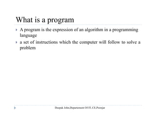
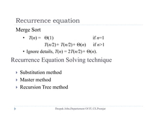
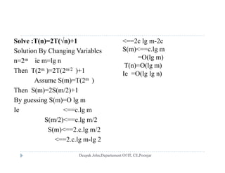
![-notation
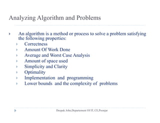
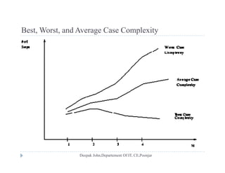
f(n)=(g(n)) there exist positive constants c and n0 where c > 0, n0 > 0
notation
For a given function g(n), the set little-omega:
such that for all n n0, we have 0 cg(n) < f(n)}.
f(n) becomes arbitrarily large relative to g(n) as n approaches infinity:
lim [f(n) / g(n)] = .
n
g(n) is a lower bound for f(n) that is not asymptotically tight.g( ) f( ) y p y g](https://image.slidesharecdn.com/anlysisanddesignofalgorithms-part1-130312001535-phpapp01/85/Anlysis-and-design-of-algorithms-part-1-22-320.jpg)

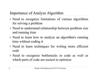
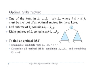
![Optimal Binary Search Trees
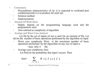
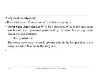
Problem
Given sequence K = k1 < k2 <··· < kn of n sorted keys, with a Given sequence K k1 k2 kn of n sorted keys, with a
search probability pi for each key ki.
Want to build a binary search tree (BST) with minimum expected
hsearch cost.
Actual cost = number of items examined.
For key k cost = depth (k )+1 where depth (k ) = depth of k in For key ki, cost = depthT(ki)+1, where depthT(ki) = depth of ki in
BST T .
• Expected Search Cost
n
pk
TE
)(depth1
]incostsearch[
i
iiT pk
1
)(depth1](https://image.slidesharecdn.com/anlysisanddesignofalgorithms-part1-130312001535-phpapp01/85/Anlysis-and-design-of-algorithms-part-1-60-320.jpg)
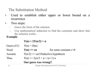
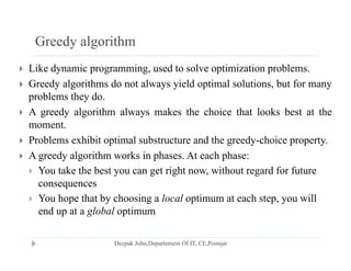
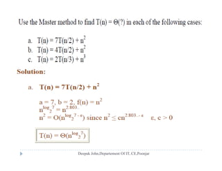
![Example
Consider 5 keys with search probabilities:
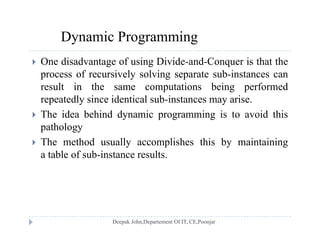
p1 = 0.25, p2 = 0.2, p3 = 0.05, p4 = 0.2, p5 = 0.3.p1 p2 p3 p4 p5
k2 i depthT(ki) depthT(ki)·pi
1 1 0.25
k1 k4
2 0 0
3 2 0.1
4 1 0.2
k3 k5
5 2 0.6
1.15
Therefore, E[search cost] = 2.15.](https://image.slidesharecdn.com/anlysisanddesignofalgorithms-part1-130312001535-phpapp01/85/Anlysis-and-design-of-algorithms-part-1-61-320.jpg)
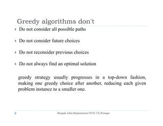
![ExampleExample
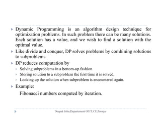
p1 = 0.25, p2 = 0.2, p3 = 0.05, p4 = 0.2, p5 = 0.3.
i depthT(ki) depthT(ki)·pi
1 1 0.25
k2
2 0 0
3 3 0.15
4 2 0.4
5 1 0 3
k1 k5
5 1 0.3
1.10
k4
Therefore, E[search cost] = 2.10.
k3 This tree turns out to be optimal for this set of keys3 This tree turns out to be optimal for this set of keys.](https://image.slidesharecdn.com/anlysisanddesignofalgorithms-part1-130312001535-phpapp01/85/Anlysis-and-design-of-algorithms-part-1-62-320.jpg)
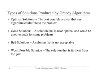
![Step 2:Recursive Solutionp
Find optimal BST for ki,...,kj, where i ≥ 1, j ≤ n, j ≥ i1.
When j = i1, the tree is empty.
Define e[i, j ] = expected search cost of optimal BST for ki,...,kj.
If j = i1, then e[i, j ] = 0.
If j ≥ i,
Select a root kr, for some i ≤ r ≤ j .
Recursively make an optimal BSTs
f k k th l ft bt d for ki,..,kr1 as the left subtree, and
for kr+1,..,kj as the right subtree.](https://image.slidesharecdn.com/anlysisanddesignofalgorithms-part1-130312001535-phpapp01/85/Anlysis-and-design-of-algorithms-part-1-65-320.jpg)
![Recursive Solution
When the OPT subtree becomes a subtree of a node:
Depth of every node in OPT subtree goes up by 1.
E t d h t i b (i j) i th f ll th Expected search cost increases by w(i,j) ,is the sum of all the
probabilities in the subtree
If kr is the root of an optimal BST for ki,..,kj :r p i j
e[i, j ] = e[i, r1] + e[r+1, j] + w(i, j).
But, we don’t know kr. Hence,](https://image.slidesharecdn.com/anlysisanddesignofalgorithms-part1-130312001535-phpapp01/85/Anlysis-and-design-of-algorithms-part-1-66-320.jpg)
![Step 3:Computing the expected search costStep 3:Computing the expected search cost
For each subproblem (i,j), store:For each subproblem (i,j), store:
expected search cost in a table use only entries e[i, j ], where j ≥
i1.
root[i, j ] = root of subtree with keys ki,..,kj, for 1 ≤ i ≤ j ≤ n.
w[1..n+1, 0..n] = sum of probabilities[ ] p
w[i, i1] = 0 for 1 ≤ i ≤ n.
w[i, j ] = w[i, j-1] + pj for 1 ≤ i ≤ j ≤ n.](https://image.slidesharecdn.com/anlysisanddesignofalgorithms-part1-130312001535-phpapp01/85/Anlysis-and-design-of-algorithms-part-1-67-320.jpg)


![Sequential Search, Unordered
I t E K h E i ith t i i d d 0 1) dInput: E, n, K, where E is an array with n entries indexed 0, …, n-1), and
K is the item sought. For simplicity, we assume that K and the entries
of E are integers, as is n.
Output: Returns ans, the location of K in E (-1 if K is not found.)
Algorithm: Step (Specification)
int seqSearch(int[] E, int n, int K)
1. int ans, index;
2 1 // A f il2. ans = -1; // Assume failure.
3. for (index = 0; index < n; index++)
4 if (K == E[index])4. if (K E[index])
5. ans = index; // Success!
6. break; // Done!;
7. return ans;](https://image.slidesharecdn.com/anlysisanddesignofalgorithms-part1-130312001535-phpapp01/75/Anlysis-and-design-of-algorithms-part-1-12-2048.jpg)
![o-notationo notation
For a given function g(n), the set little-o:
f(n)=o(g(n)) there exist positive constants c and n0 where c > 0, n0 > 0
such that for all n n0, we have 0 f(n) < cg(n).
f(n) becomes insignificant relative to g(n) as n approaches infinity:f( ) g g( ) pp y
lim [f(n) / g(n)] = 0
n
g(n) is an upper bound for f(n) that is not asymptotically tightg(n) is an upper bound for f(n) that is not asymptotically tight.](https://image.slidesharecdn.com/anlysisanddesignofalgorithms-part1-130312001535-phpapp01/75/Anlysis-and-design-of-algorithms-part-1-21-2048.jpg)
![-notation
f(n)=(g(n)) there exist positive constants c and n0 where c > 0, n0 > 0
notation
For a given function g(n), the set little-omega:
such that for all n n0, we have 0 cg(n) < f(n)}.
f(n) becomes arbitrarily large relative to g(n) as n approaches infinity:
lim [f(n) / g(n)] = .
n
g(n) is a lower bound for f(n) that is not asymptotically tight.g( ) f( ) y p y g](https://image.slidesharecdn.com/anlysisanddesignofalgorithms-part1-130312001535-phpapp01/75/Anlysis-and-design-of-algorithms-part-1-22-2048.jpg)

![Optimal Binary Search Trees
Problem
Given sequence K = k1 < k2 <··· < kn of n sorted keys, with a Given sequence K k1 k2 kn of n sorted keys, with a
search probability pi for each key ki.
Want to build a binary search tree (BST) with minimum expected
hsearch cost.
Actual cost = number of items examined.
For key k cost = depth (k )+1 where depth (k ) = depth of k in For key ki, cost = depthT(ki)+1, where depthT(ki) = depth of ki in
BST T .
• Expected Search Cost
n
pk
TE
)(depth1
]incostsearch[
i
iiT pk
1
)(depth1](https://image.slidesharecdn.com/anlysisanddesignofalgorithms-part1-130312001535-phpapp01/75/Anlysis-and-design-of-algorithms-part-1-60-2048.jpg)
![Example
Consider 5 keys with search probabilities:
p1 = 0.25, p2 = 0.2, p3 = 0.05, p4 = 0.2, p5 = 0.3.p1 p2 p3 p4 p5
k2 i depthT(ki) depthT(ki)·pi
1 1 0.25
k1 k4
2 0 0
3 2 0.1
4 1 0.2
k3 k5
5 2 0.6
1.15
Therefore, E[search cost] = 2.15.](https://image.slidesharecdn.com/anlysisanddesignofalgorithms-part1-130312001535-phpapp01/75/Anlysis-and-design-of-algorithms-part-1-61-2048.jpg)
![ExampleExample
p1 = 0.25, p2 = 0.2, p3 = 0.05, p4 = 0.2, p5 = 0.3.
i depthT(ki) depthT(ki)·pi
1 1 0.25
k2
2 0 0
3 3 0.15
4 2 0.4
5 1 0 3
k1 k5
5 1 0.3
1.10
k4
Therefore, E[search cost] = 2.10.
k3 This tree turns out to be optimal for this set of keys3 This tree turns out to be optimal for this set of keys.](https://image.slidesharecdn.com/anlysisanddesignofalgorithms-part1-130312001535-phpapp01/75/Anlysis-and-design-of-algorithms-part-1-62-2048.jpg)
![Step 2:Recursive Solutionp
Find optimal BST for ki,...,kj, where i ≥ 1, j ≤ n, j ≥ i1.
When j = i1, the tree is empty.
Define e[i, j ] = expected search cost of optimal BST for ki,...,kj.
If j = i1, then e[i, j ] = 0.
If j ≥ i,
Select a root kr, for some i ≤ r ≤ j .
Recursively make an optimal BSTs
f k k th l ft bt d for ki,..,kr1 as the left subtree, and
for kr+1,..,kj as the right subtree.](https://image.slidesharecdn.com/anlysisanddesignofalgorithms-part1-130312001535-phpapp01/75/Anlysis-and-design-of-algorithms-part-1-65-2048.jpg)
![Recursive Solution
When the OPT subtree becomes a subtree of a node:
Depth of every node in OPT subtree goes up by 1.
E t d h t i b (i j) i th f ll th Expected search cost increases by w(i,j) ,is the sum of all the
probabilities in the subtree
If kr is the root of an optimal BST for ki,..,kj :r p i j
e[i, j ] = e[i, r1] + e[r+1, j] + w(i, j).
But, we don’t know kr. Hence,](https://image.slidesharecdn.com/anlysisanddesignofalgorithms-part1-130312001535-phpapp01/75/Anlysis-and-design-of-algorithms-part-1-66-2048.jpg)
![Step 3:Computing the expected search costStep 3:Computing the expected search cost
For each subproblem (i,j), store:For each subproblem (i,j), store:
expected search cost in a table use only entries e[i, j ], where j ≥
i1.
root[i, j ] = root of subtree with keys ki,..,kj, for 1 ≤ i ≤ j ≤ n.
w[1..n+1, 0..n] = sum of probabilities[ ] p
w[i, i1] = 0 for 1 ≤ i ≤ n.
w[i, j ] = w[i, j-1] + pj for 1 ≤ i ≤ j ≤ n.](https://image.slidesharecdn.com/anlysisanddesignofalgorithms-part1-130312001535-phpapp01/75/Anlysis-and-design-of-algorithms-part-1-67-2048.jpg)


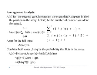
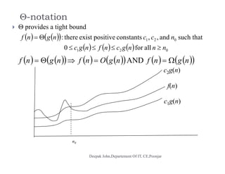
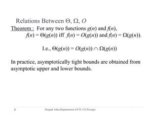
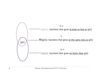
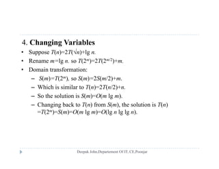
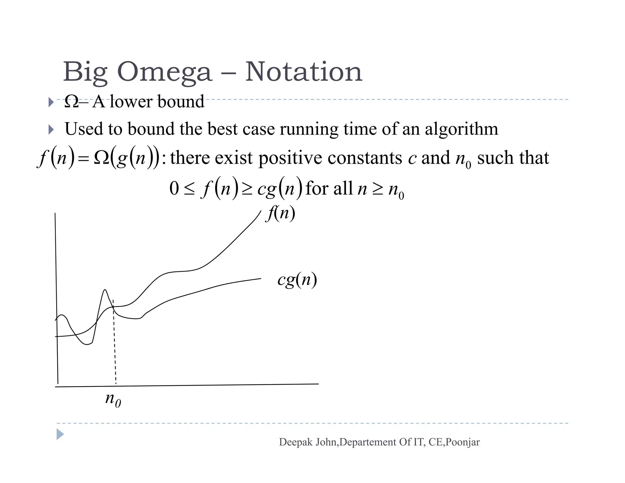
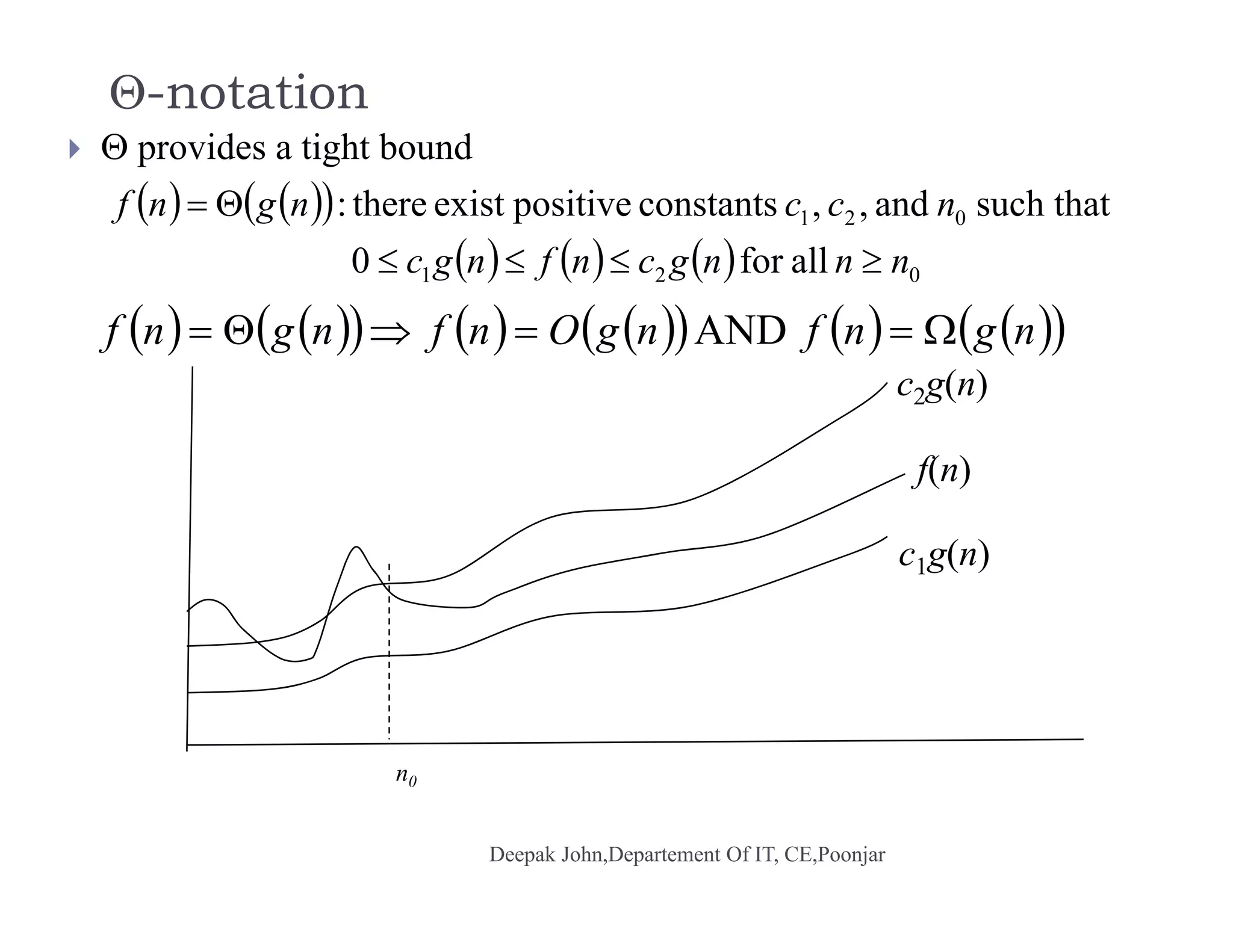
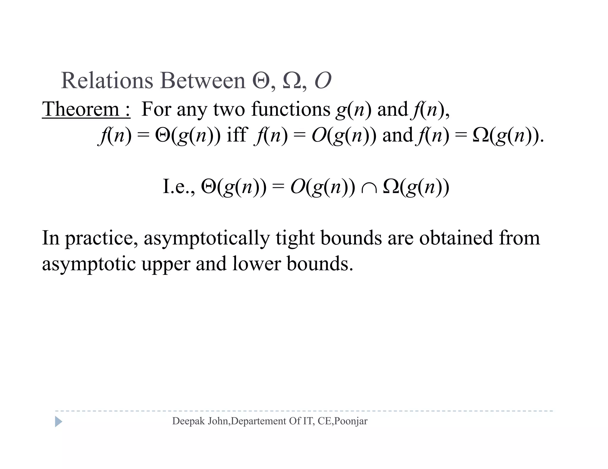
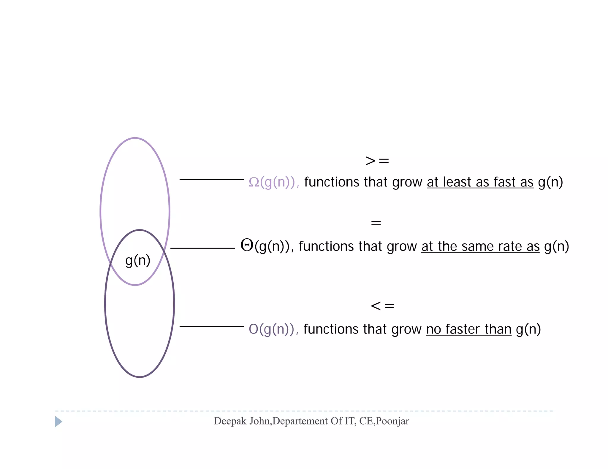
The document provides an in-depth analysis of algorithms, defining their structures and importance in problem-solving within computer applications. It covers the concepts of algorithm design, complexity analysis, including best, worst, and average case scenarios, as well as asymptotic notations such as Big O, Omega, and Theta for measuring algorithm efficiency. Additionally, it explains recursive algorithms and their analysis through techniques like the substitution method and the master method.
Analysis and Design of Algorithms, by Deepak John, focusing on algorithmic foundations.
Algorithms as procedures transforming input to output; programs as algorithm expressions in code.
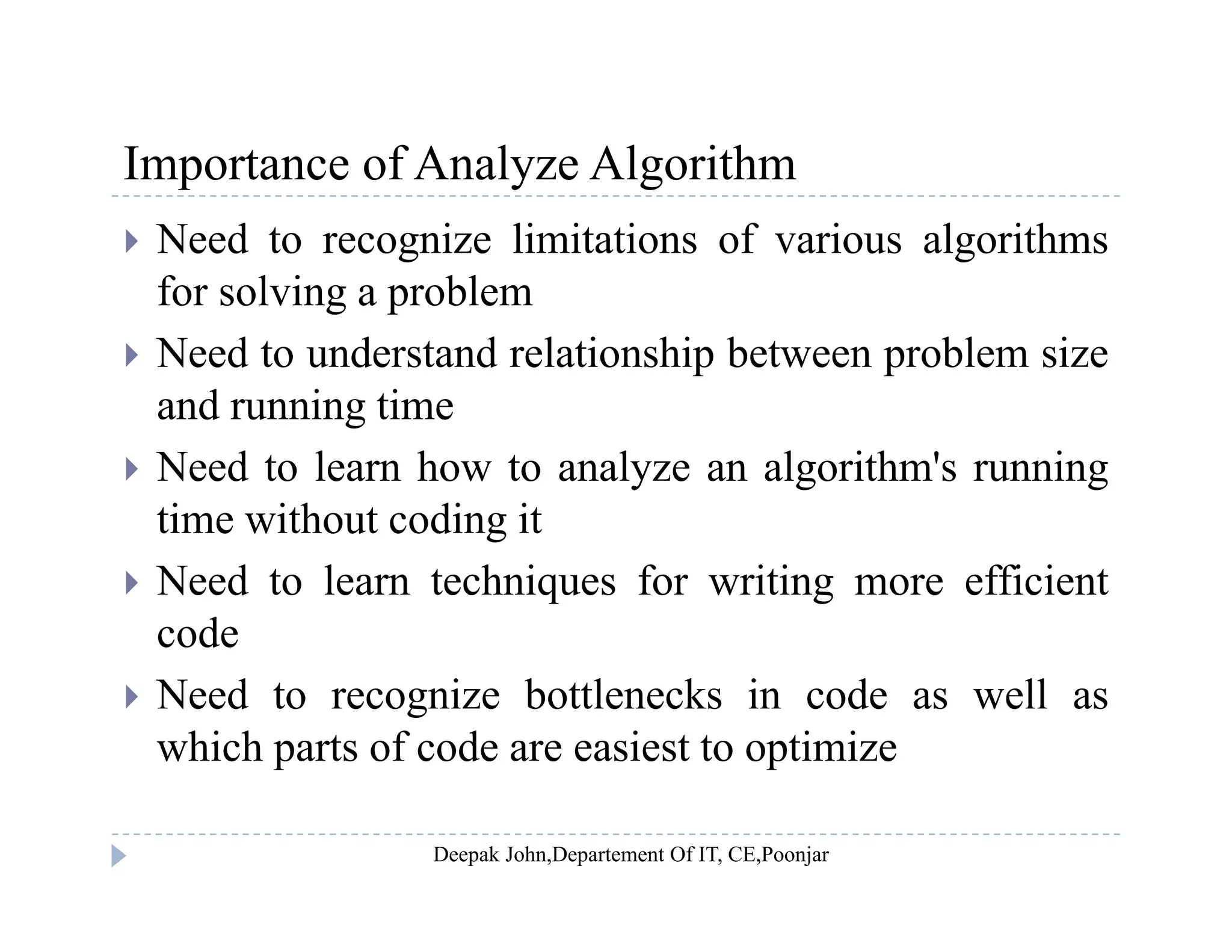
The necessity of understanding algorithm limits, size vs. time relationships, efficiency, and optimization.
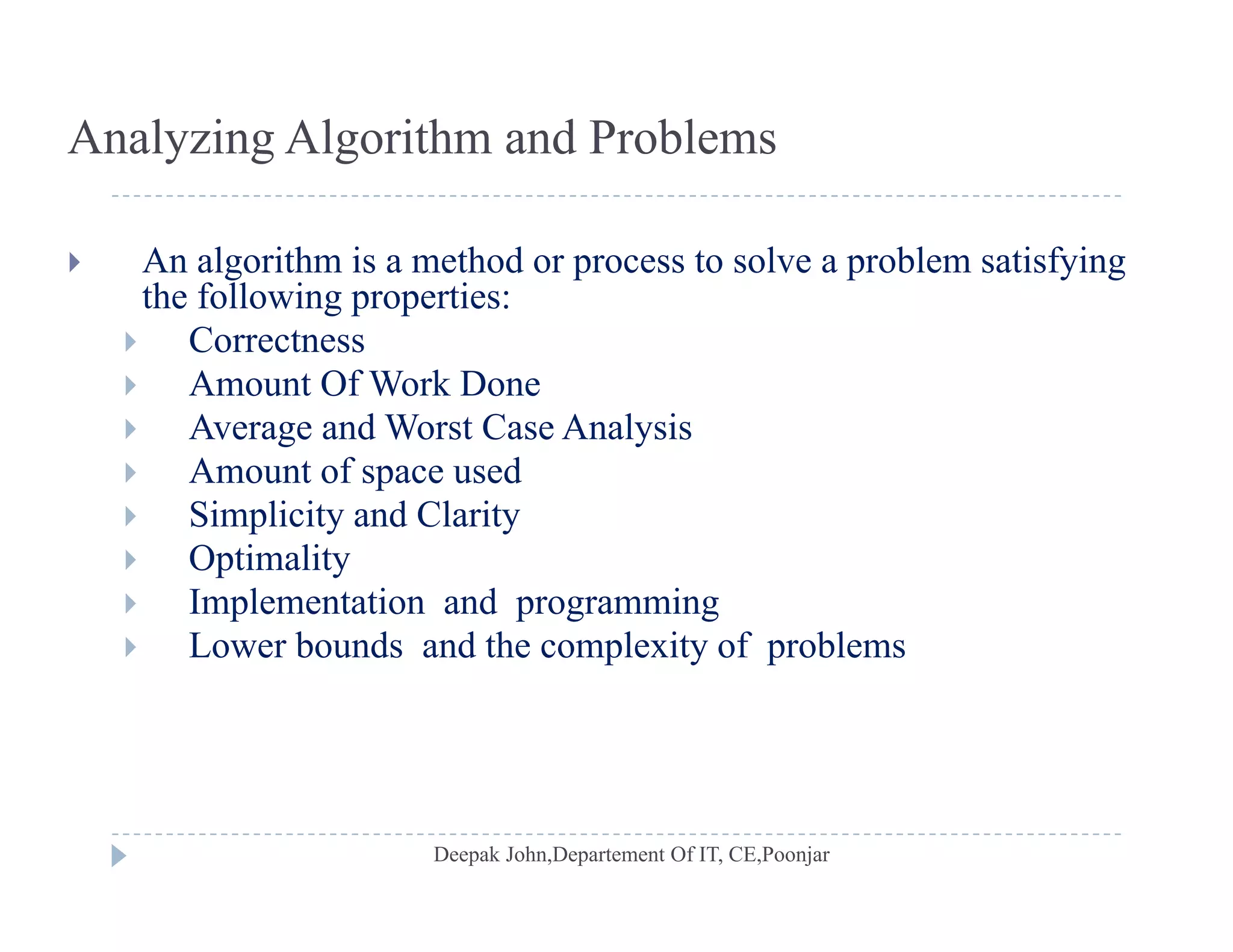
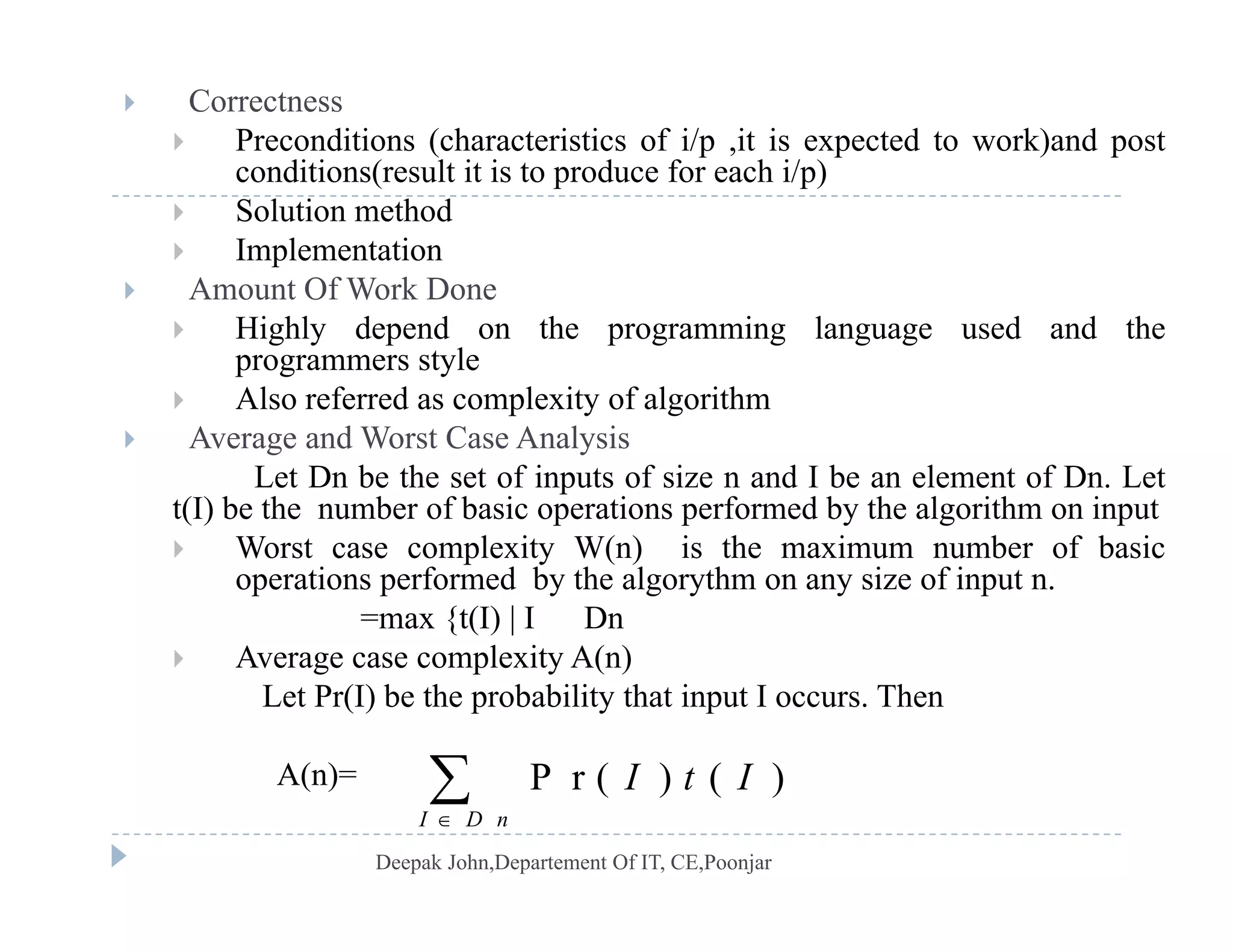
Key properties for analyzing algorithms: correctness, work done, case analysis, space usage, and complexity.
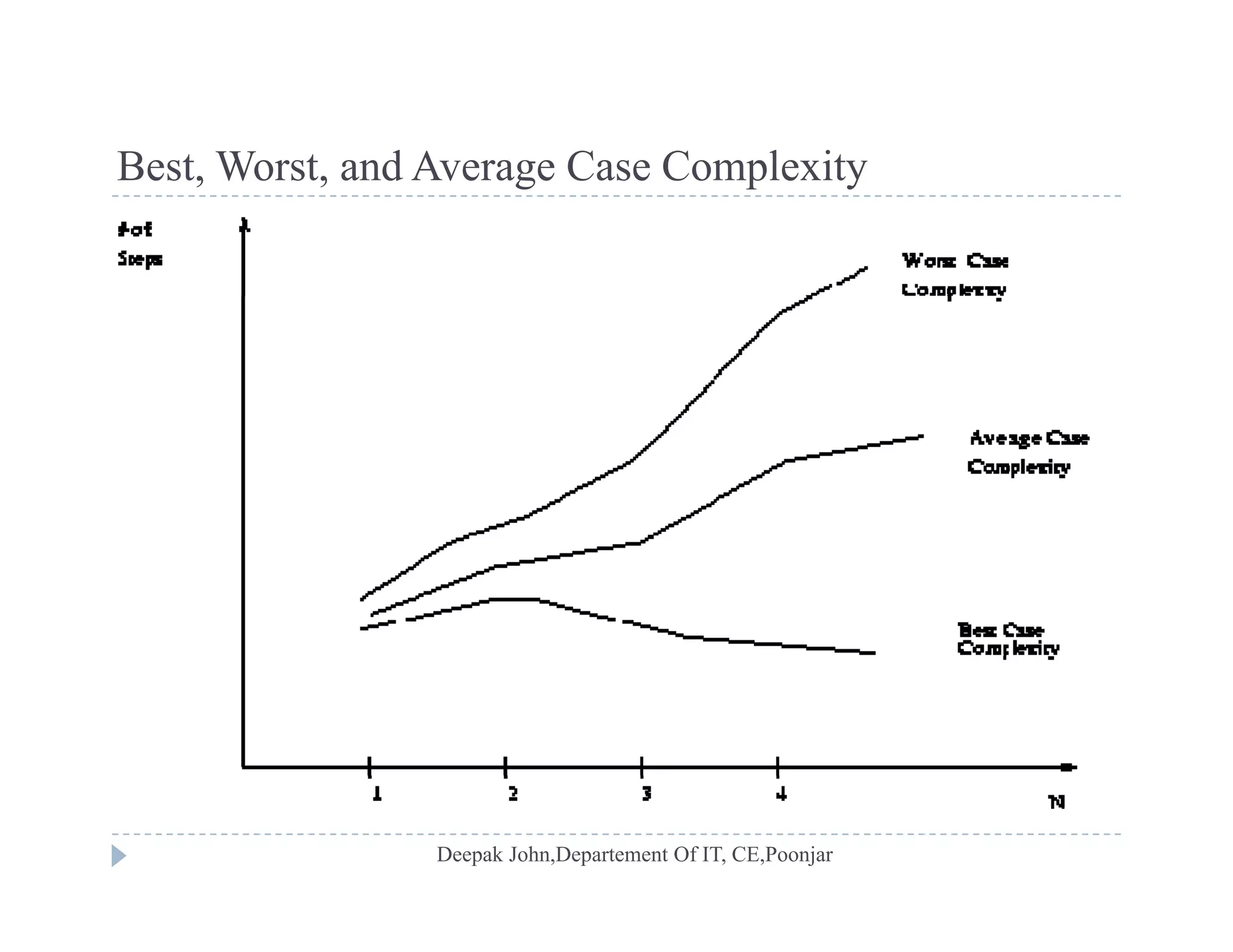
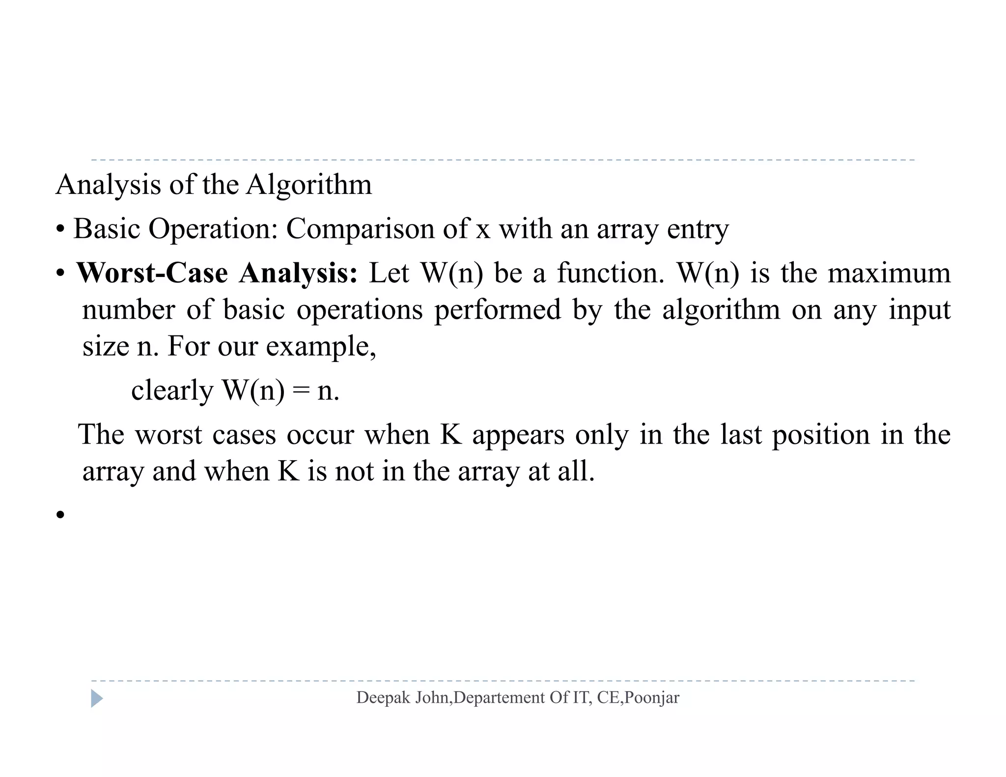
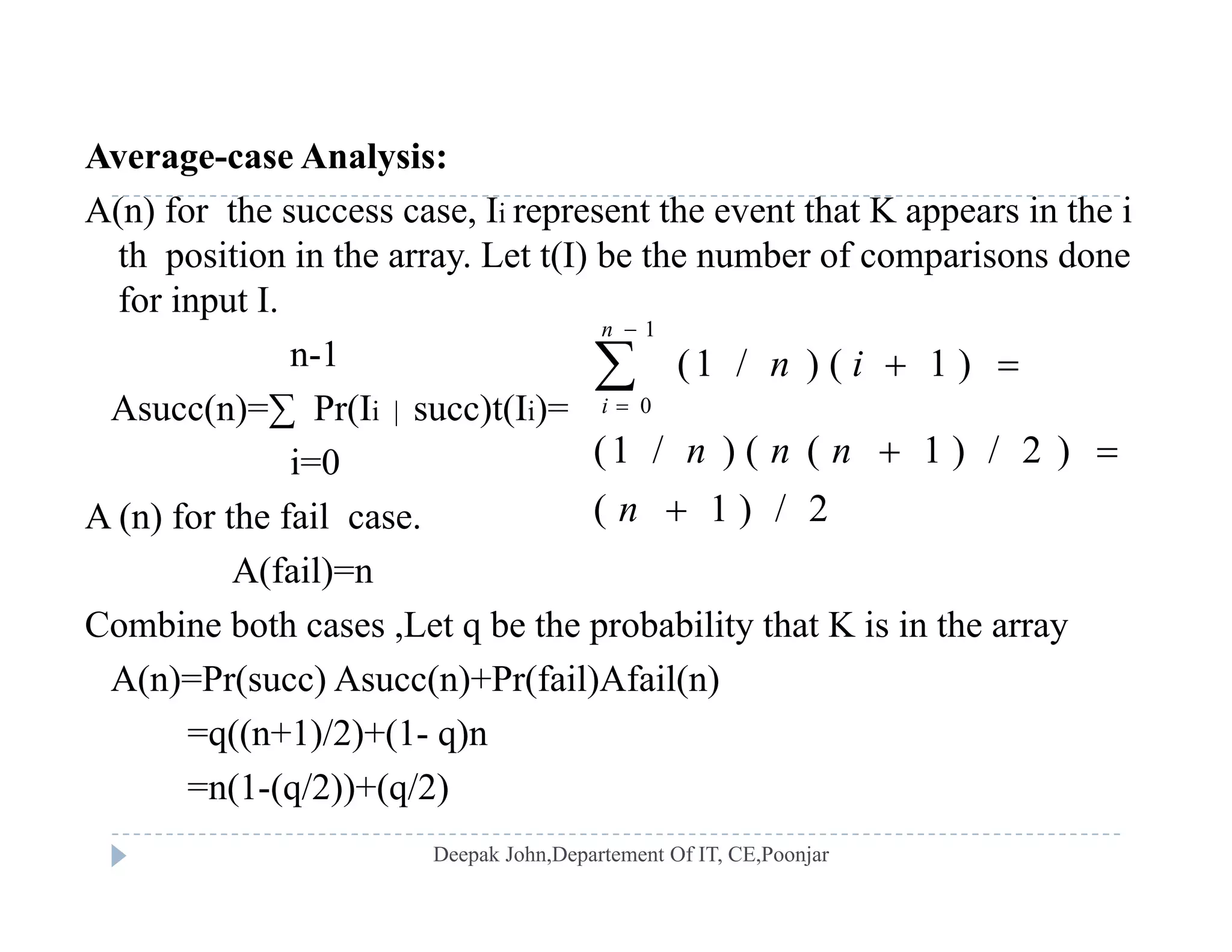
Discussion of worst, best, and average case complexities for algorithms in context.
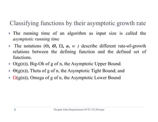
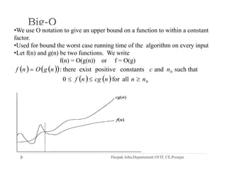
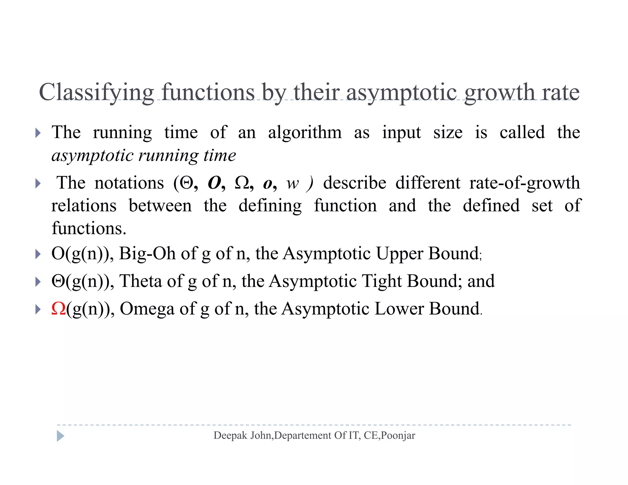
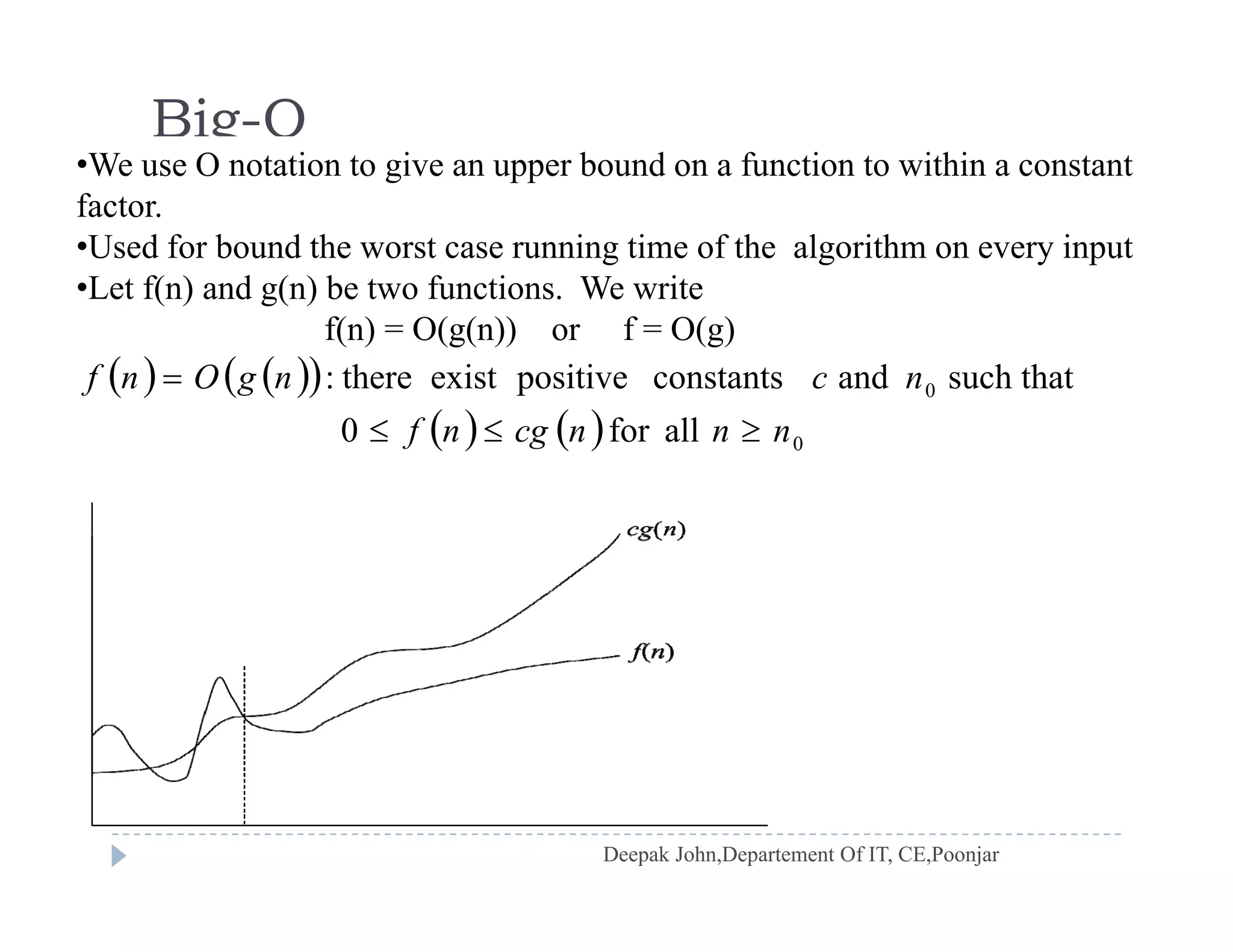
Worst-case, average-case complexities with examples of searching algorithms and their analysis.Classifications of functions based on growth rates: Big O, Theta, Omega, little o, and little ω.
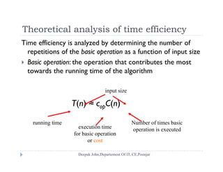
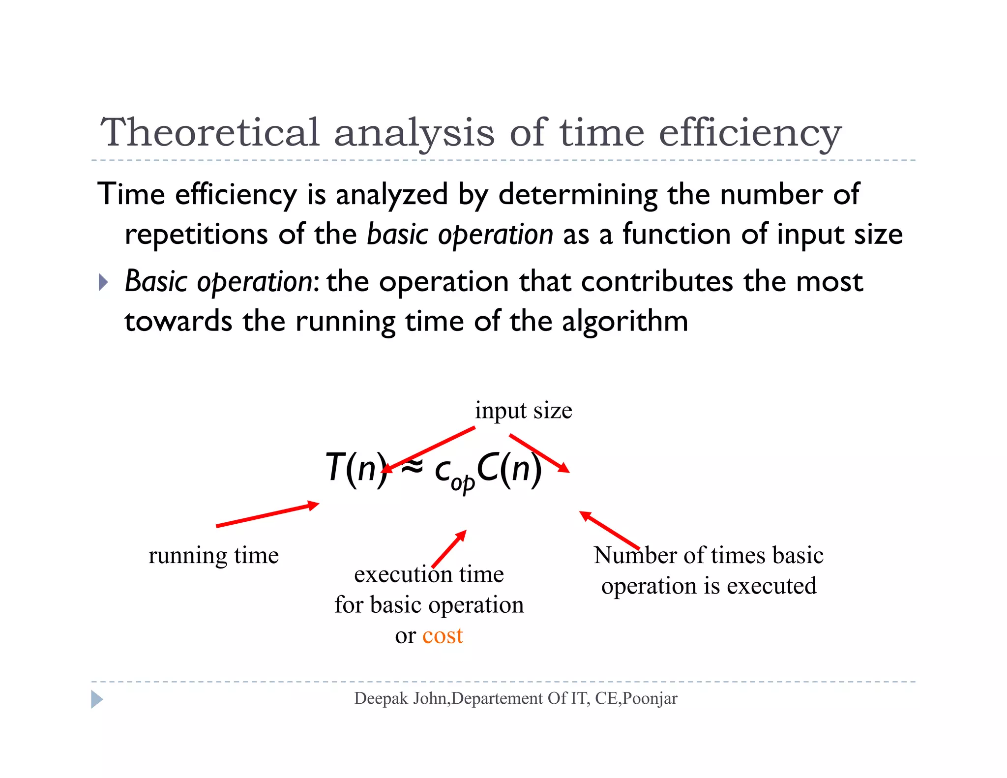
Understanding time efficiency by counting basic operations' repetitions relative to input size.
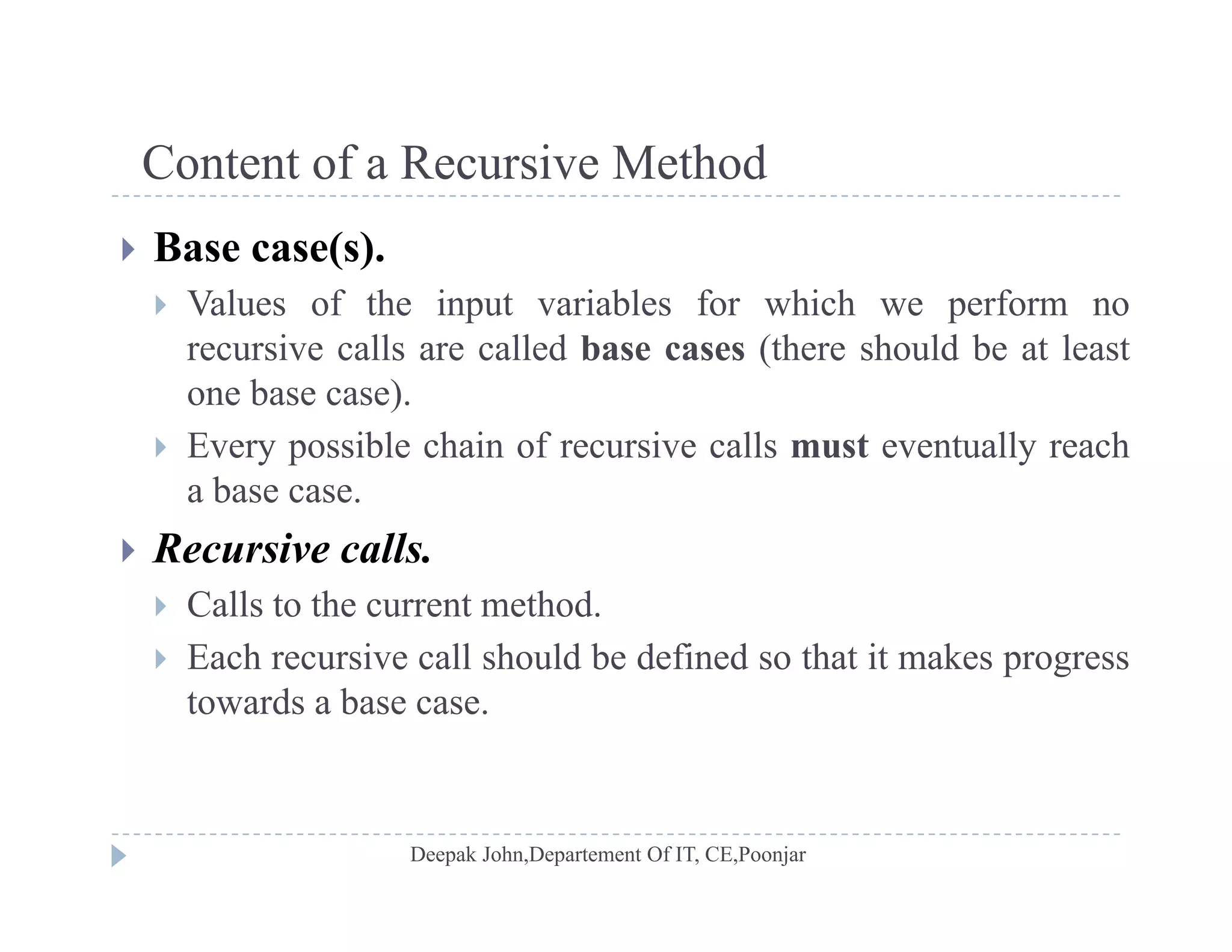
Definition of recursive methods and critical base cases required for effective recursion.
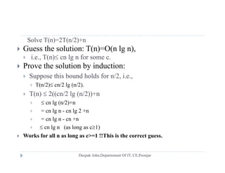
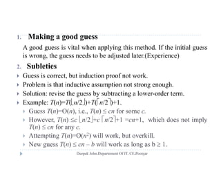
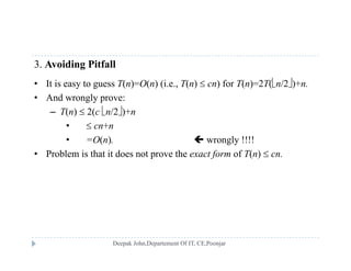
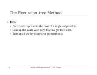
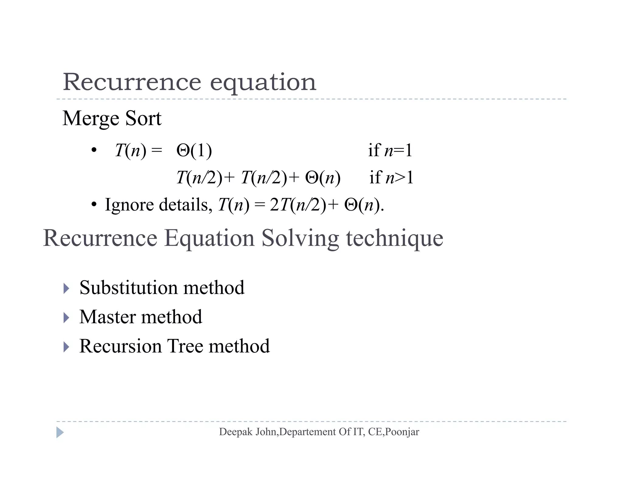
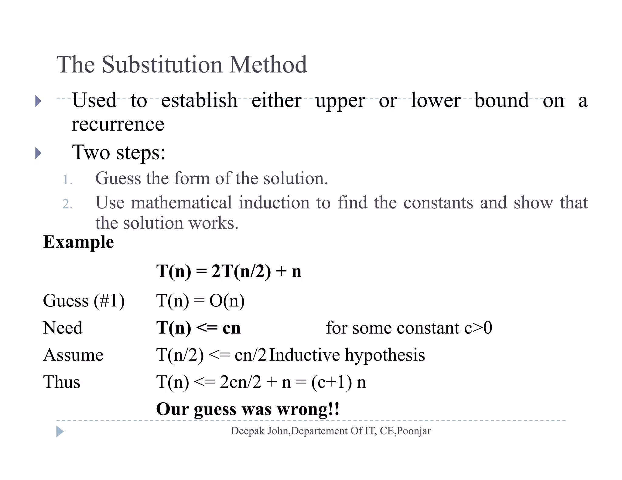
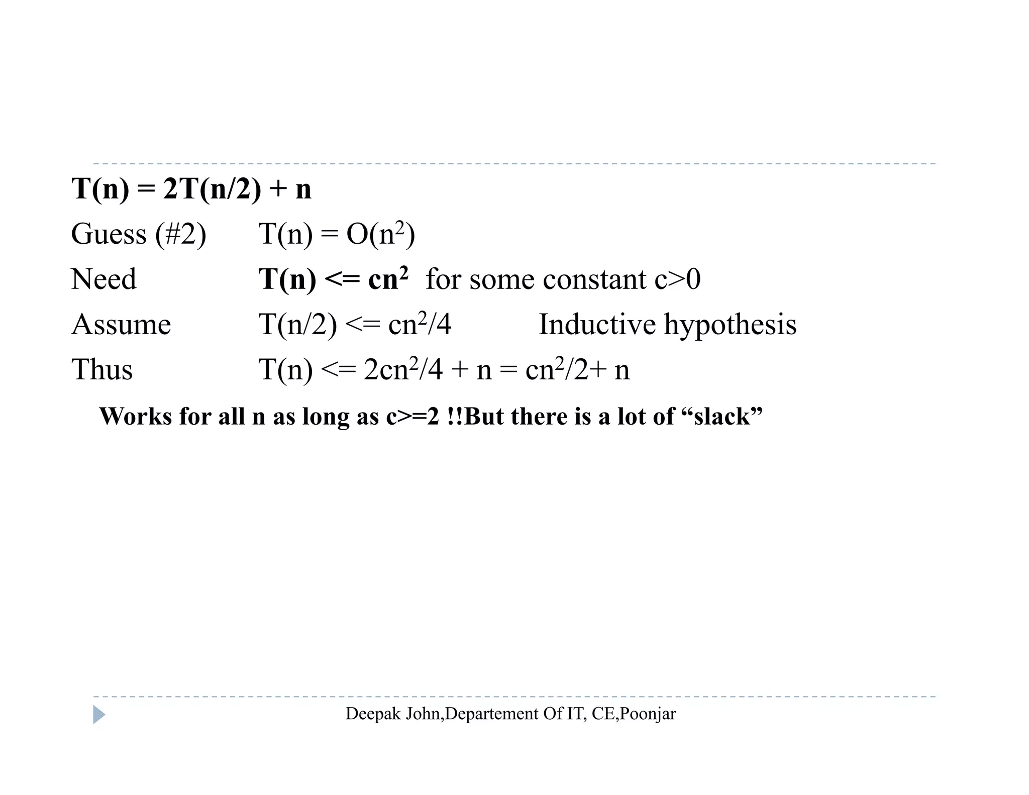
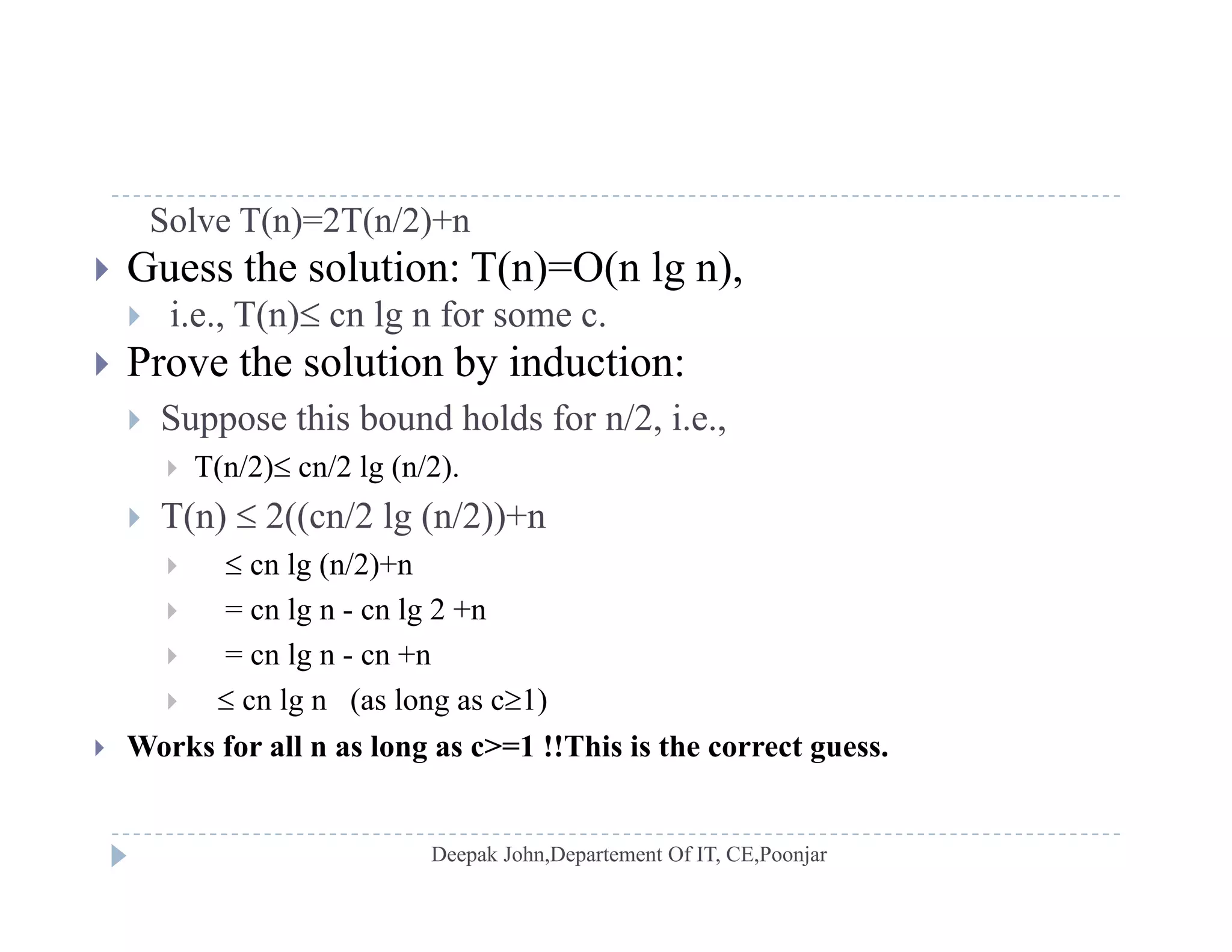
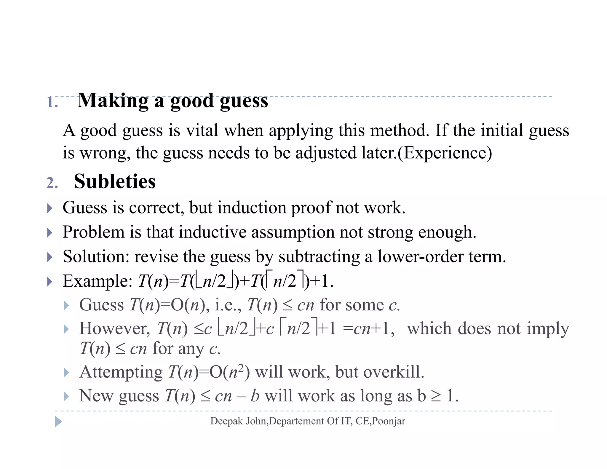
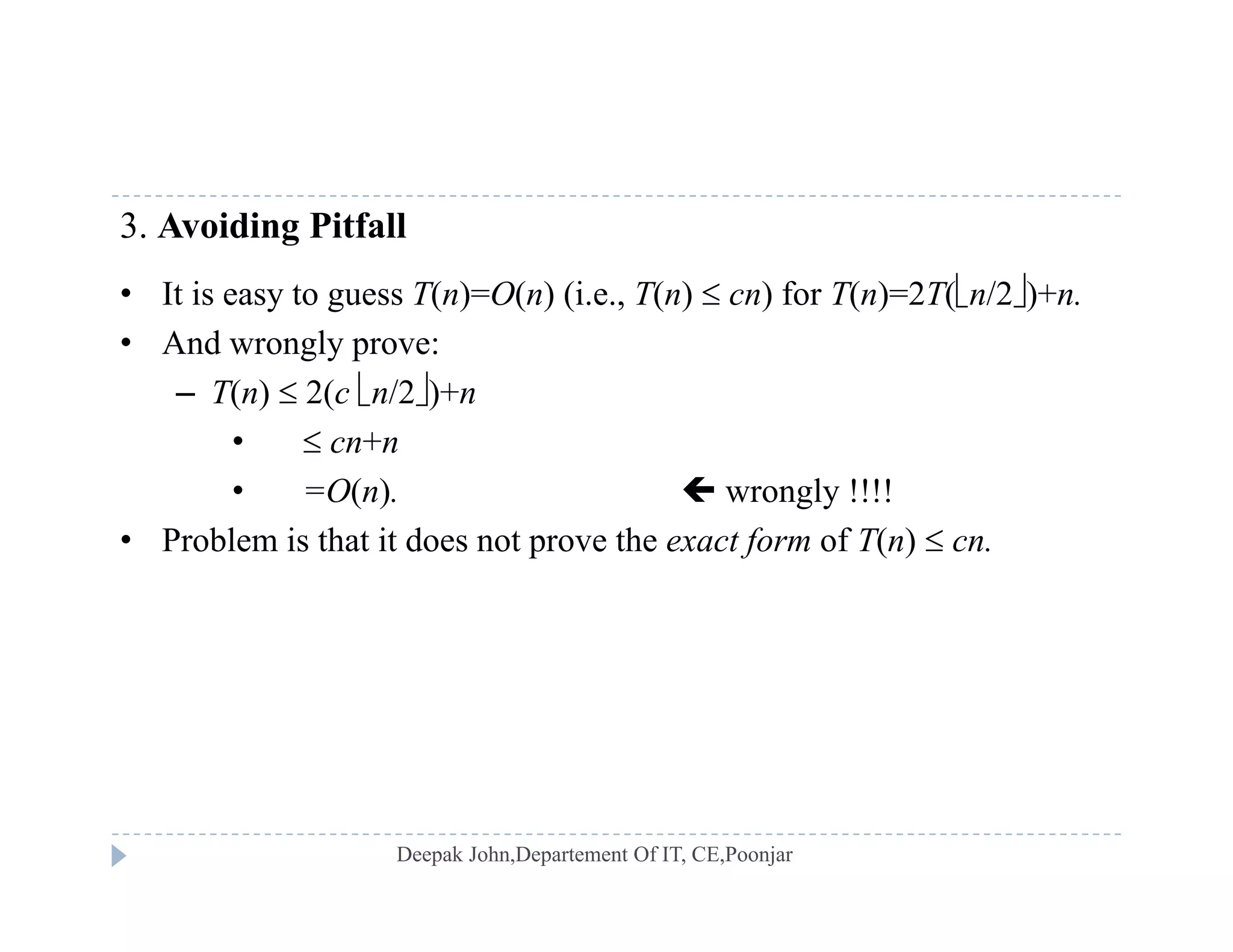
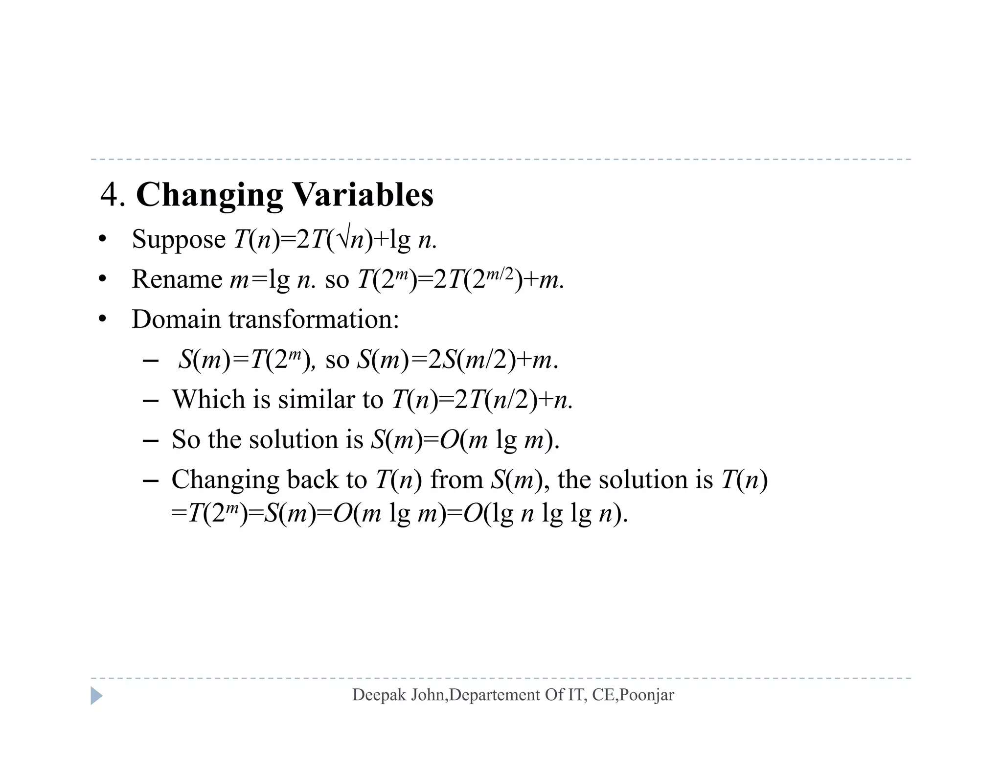
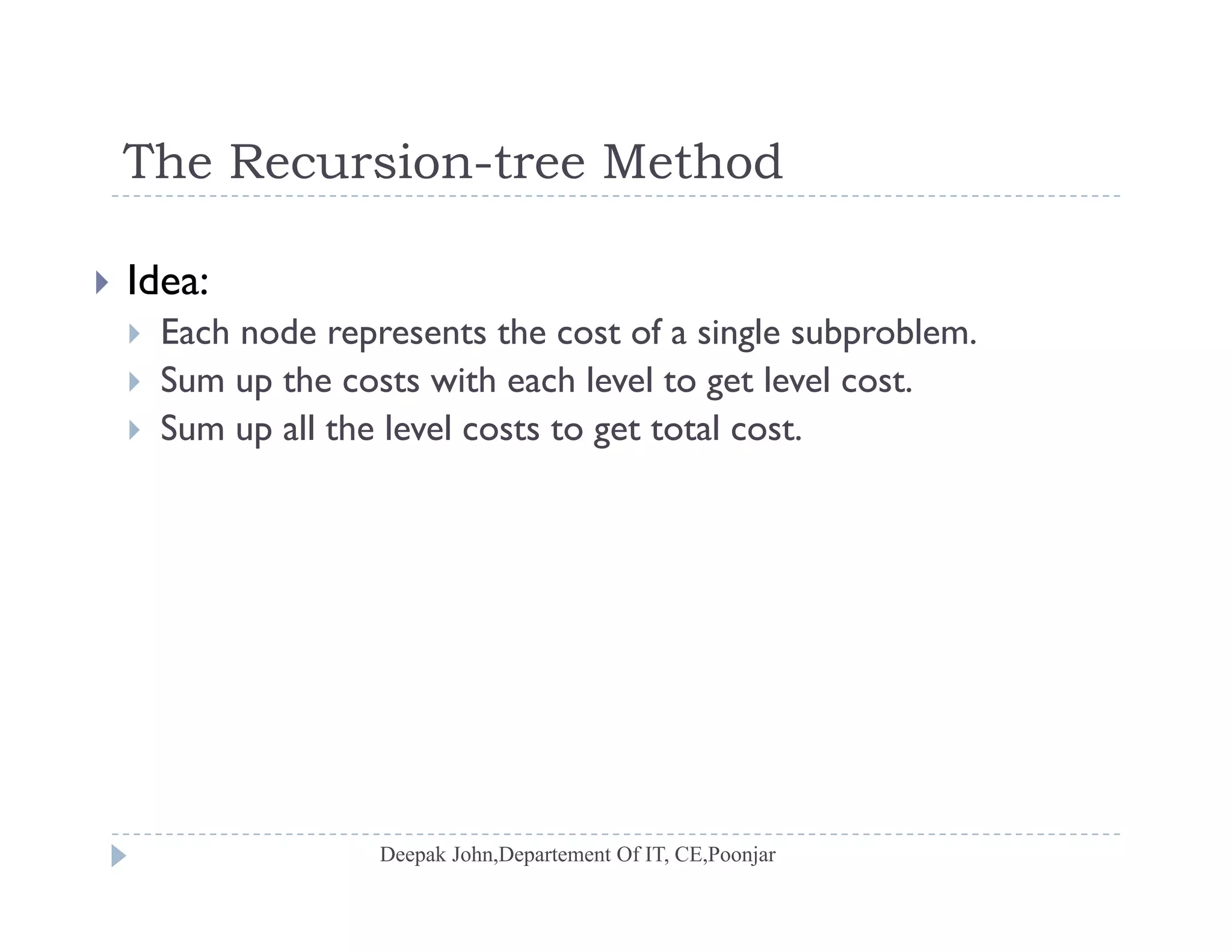
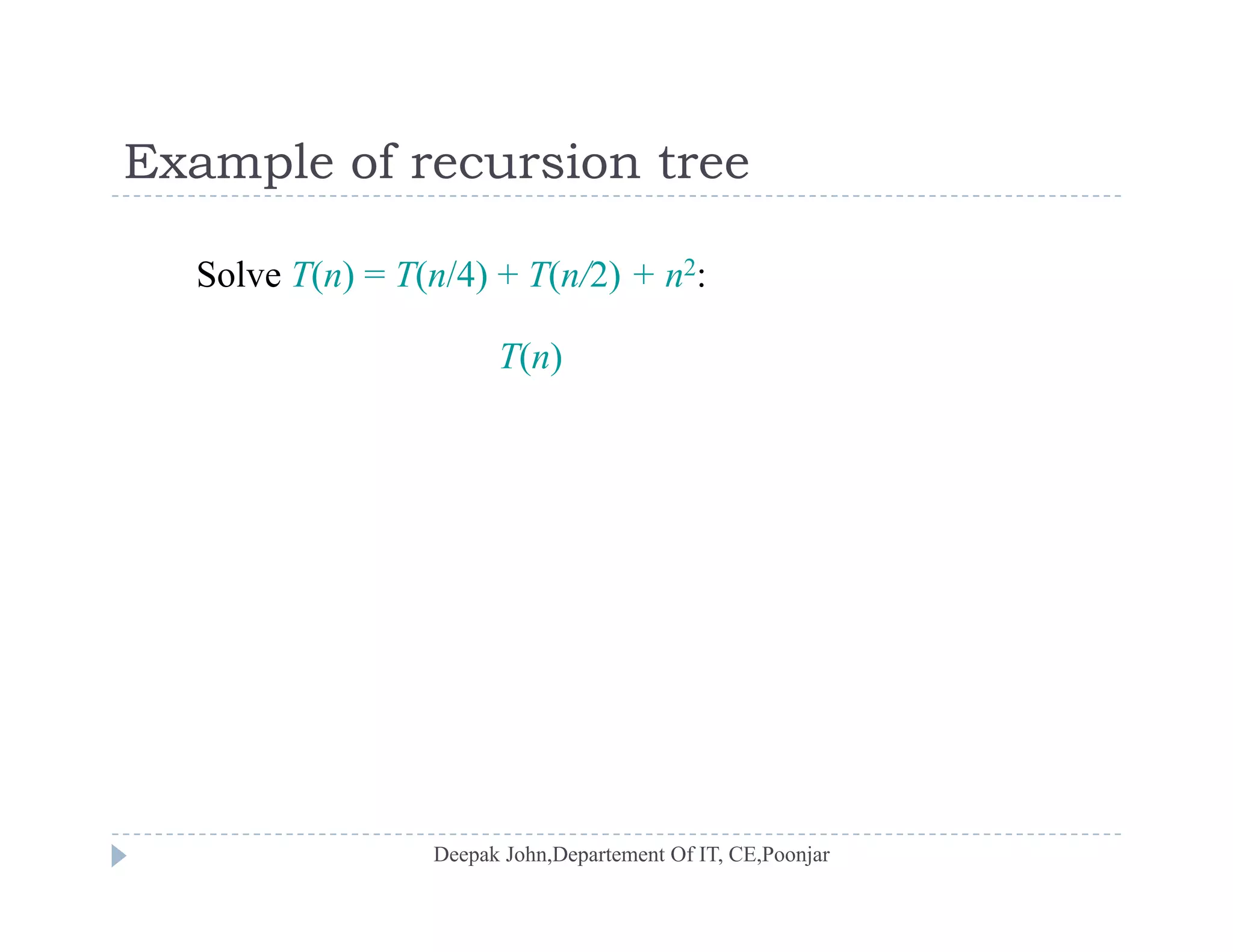
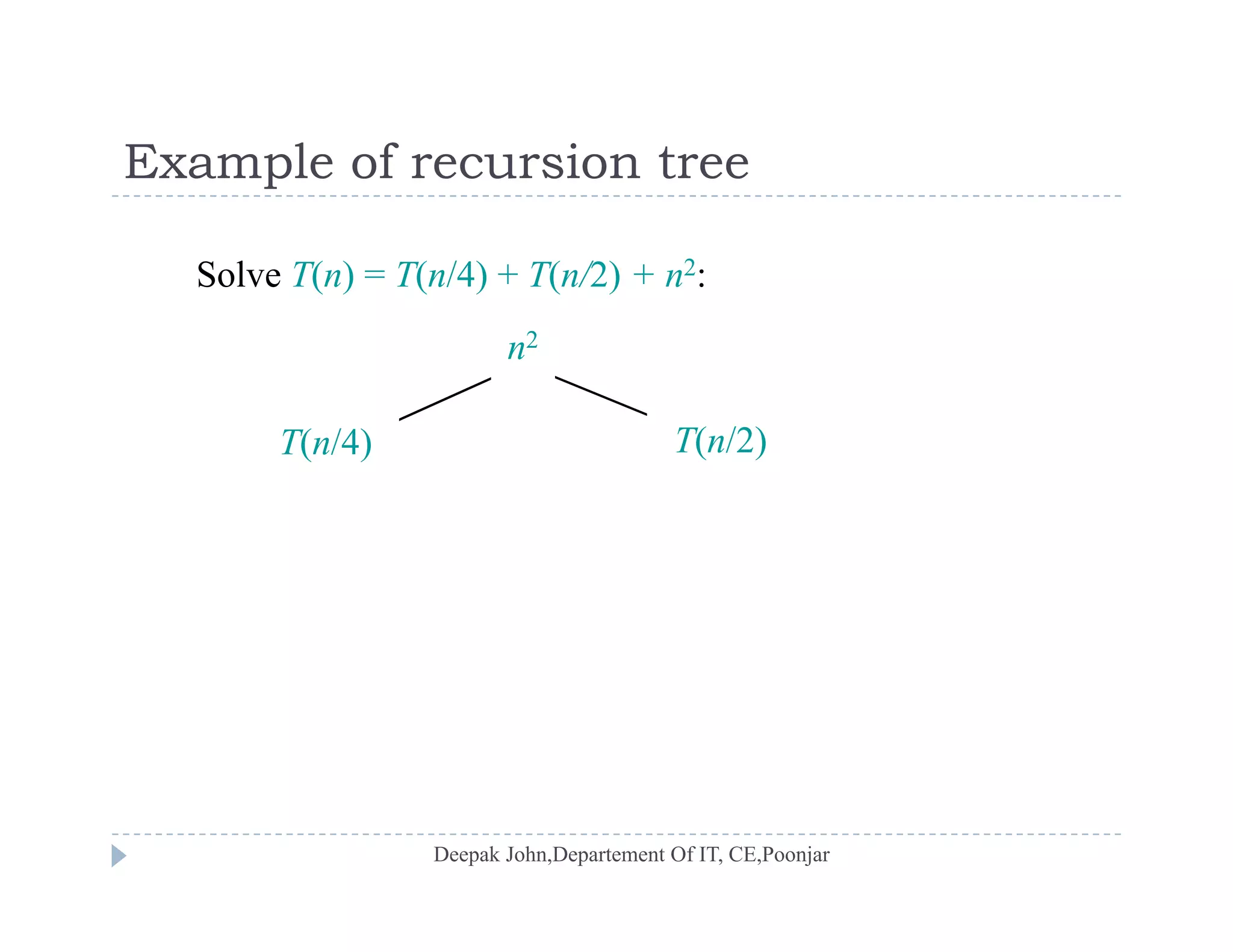
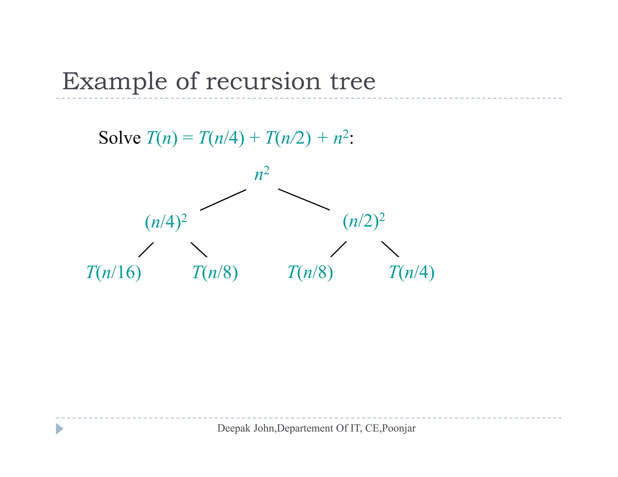
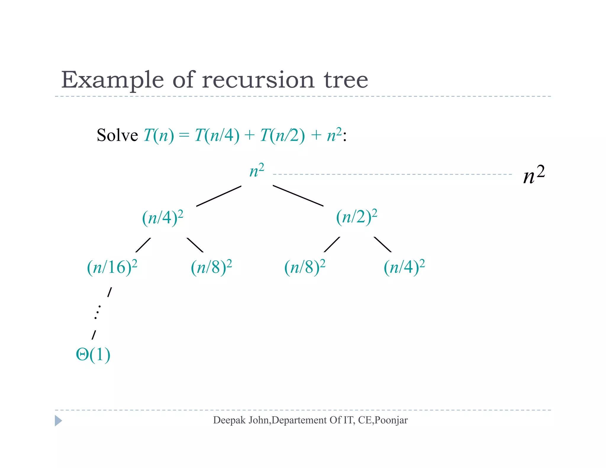
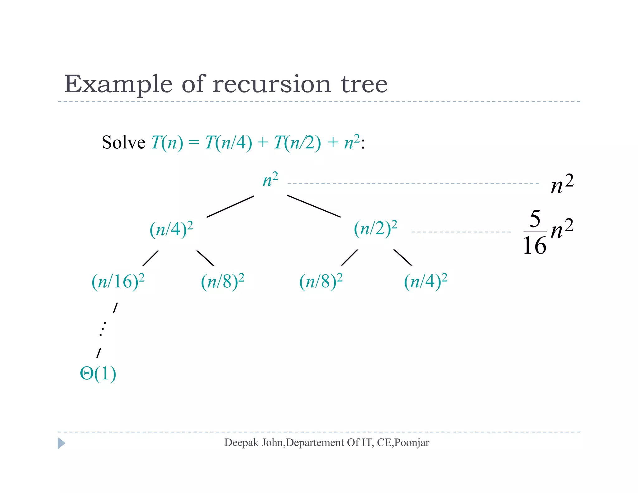
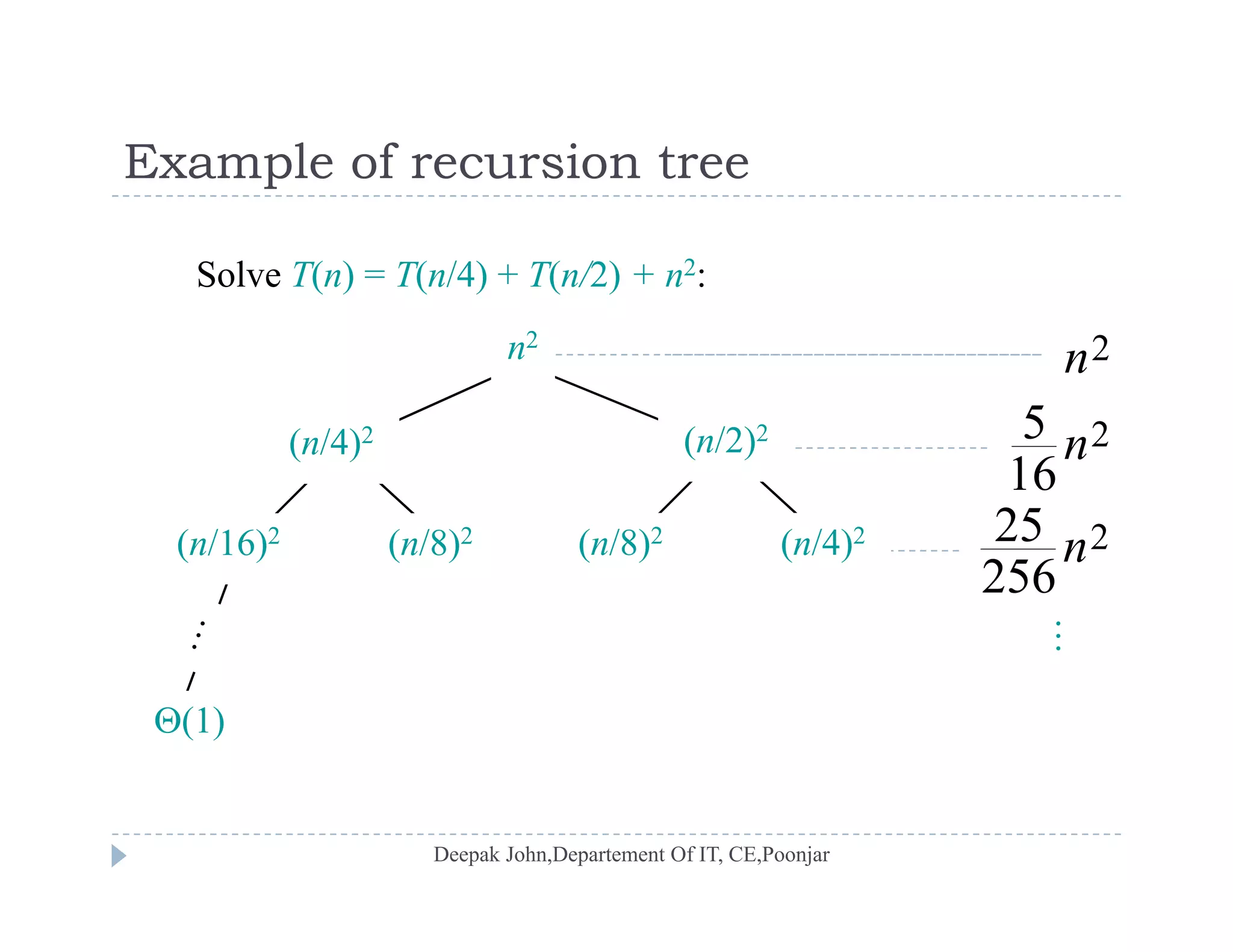
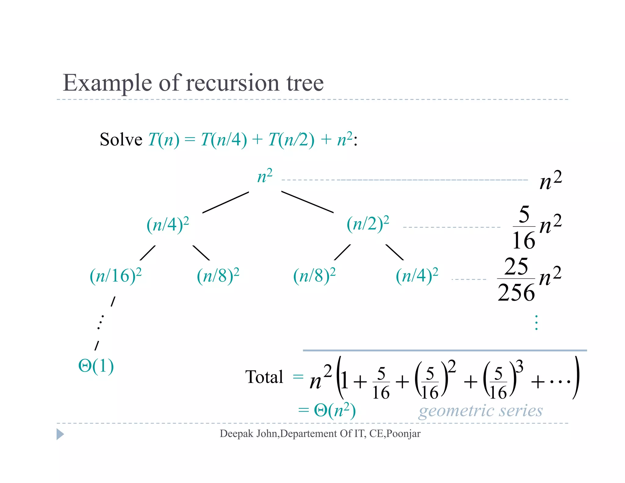
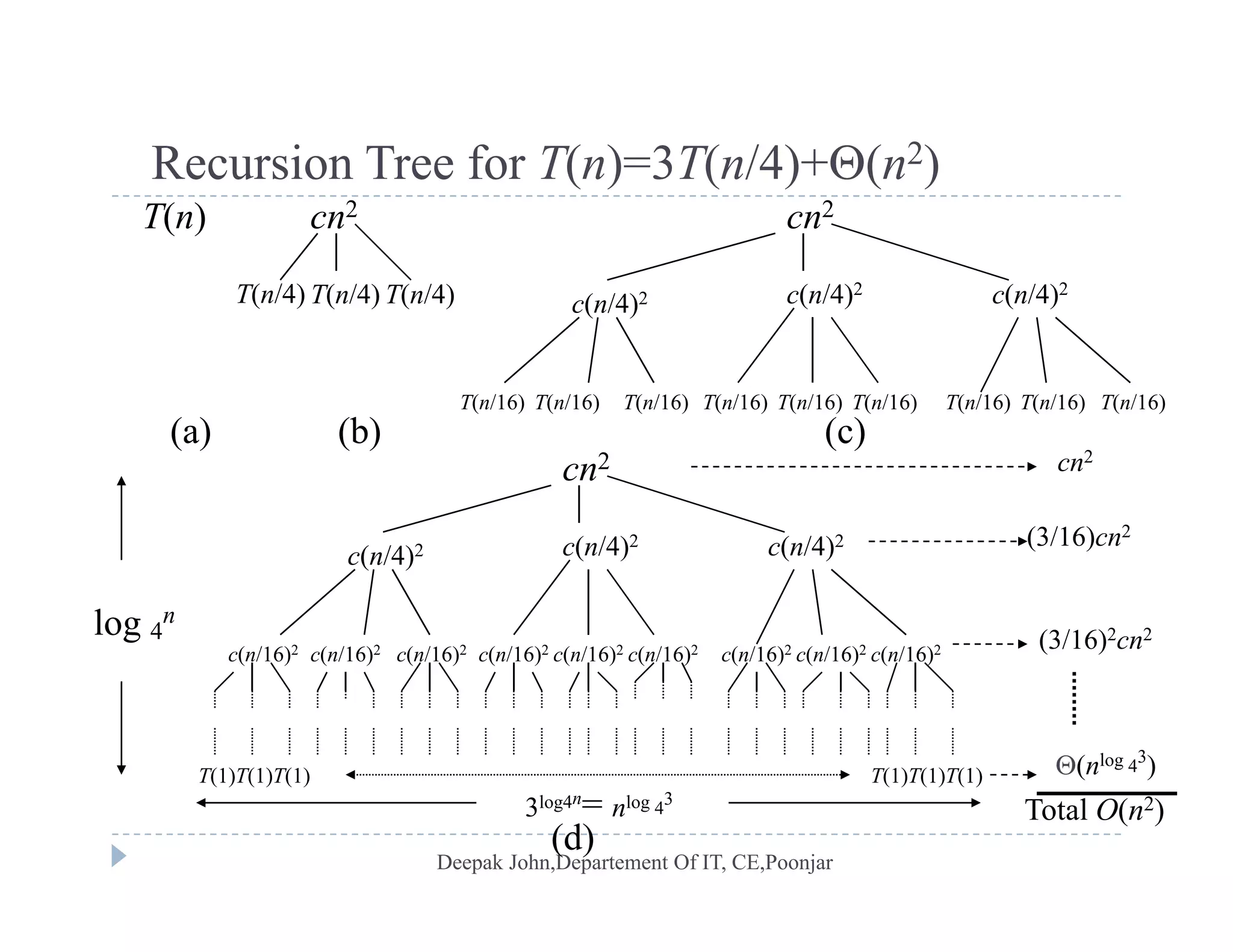
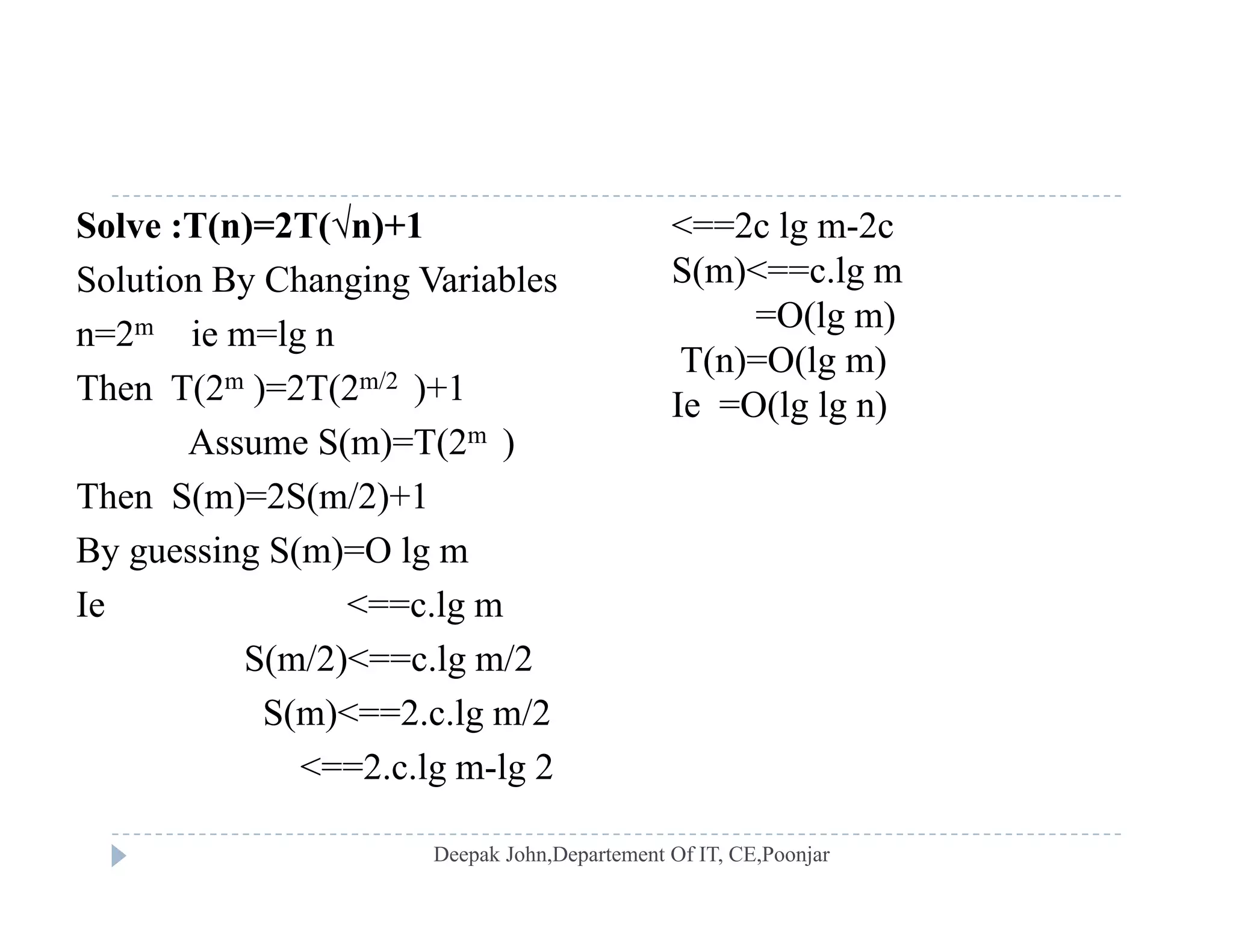
Techniques for solving recurrence relations, including substitution and tree method approaches.
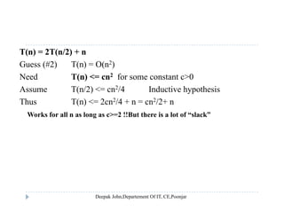
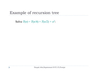
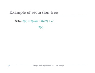
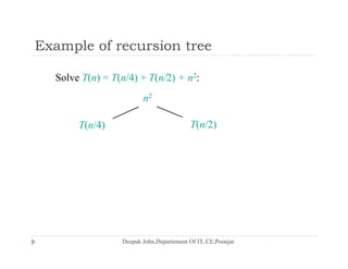
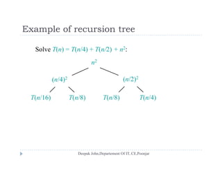
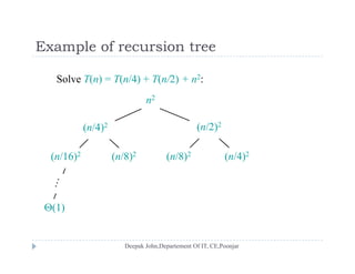
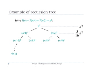
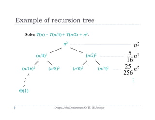
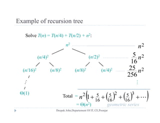
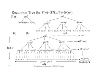
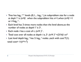
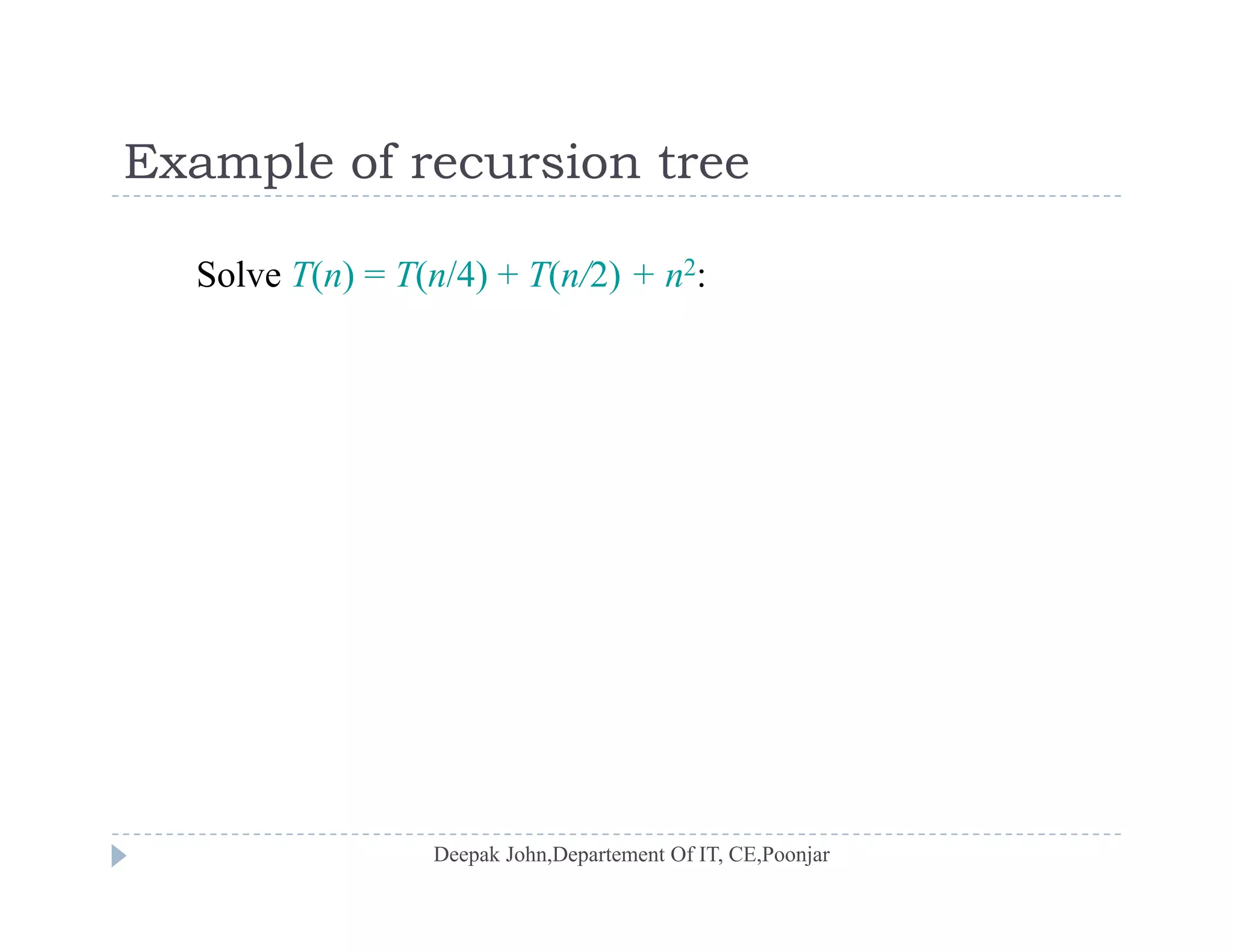
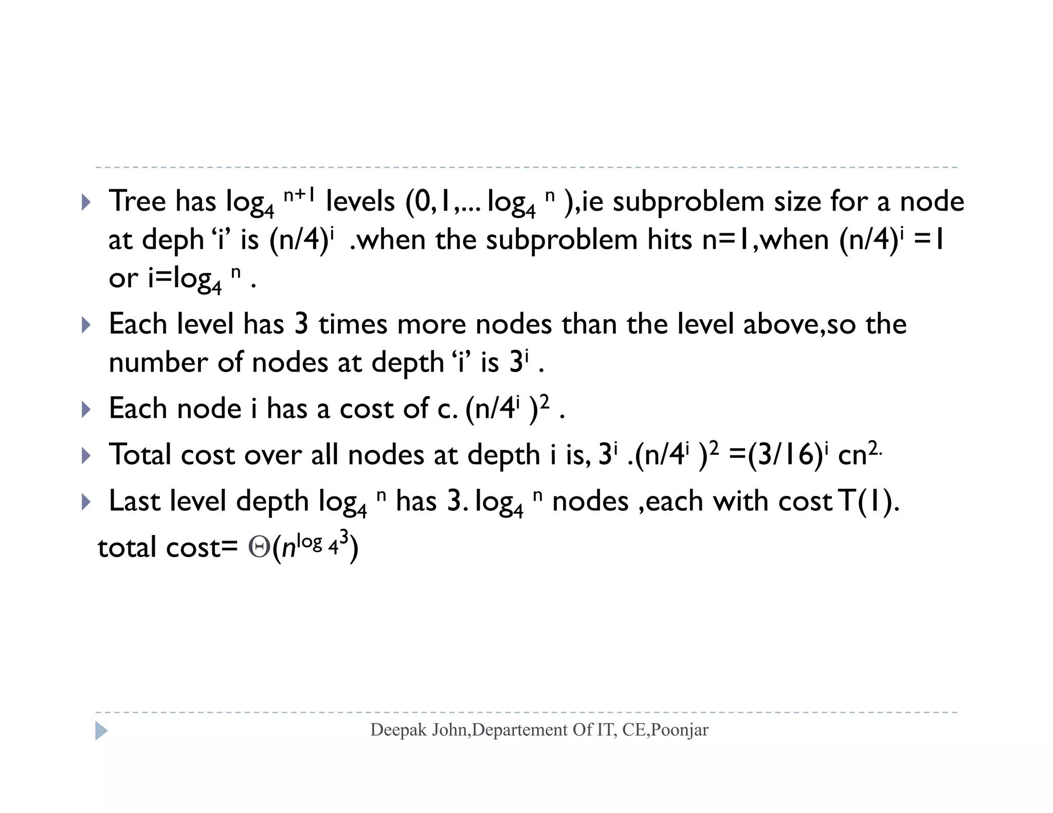
Illustrating the recursion tree method for understanding costs of recursive algorithms, exemplified.
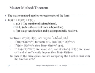
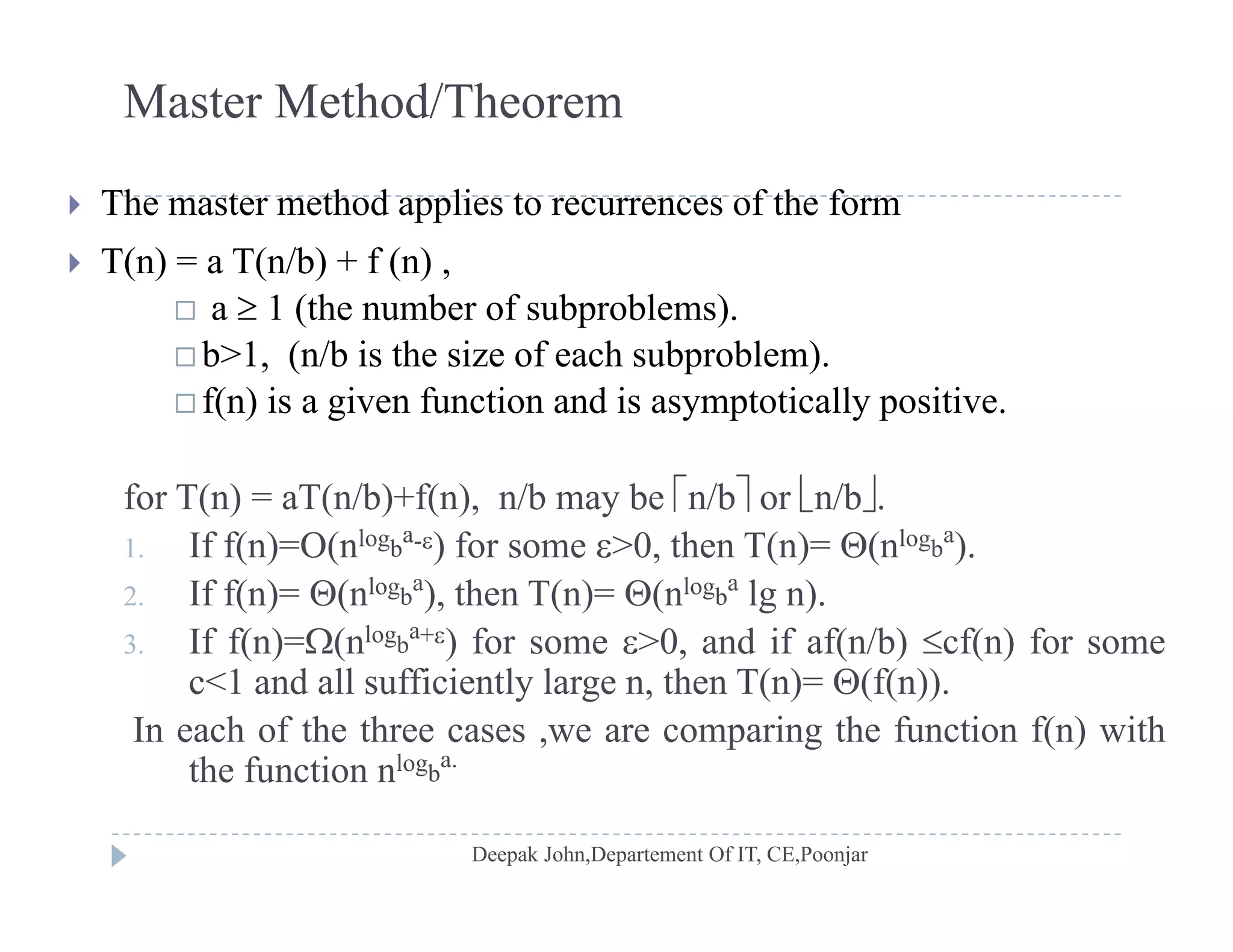
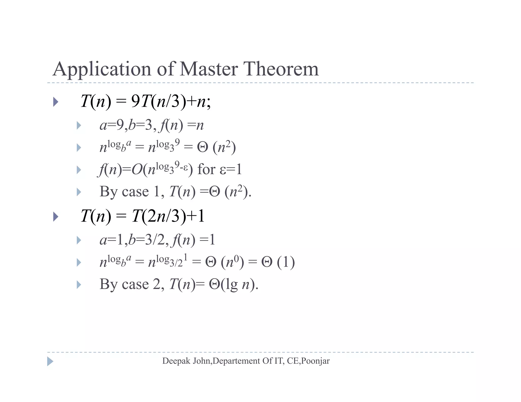
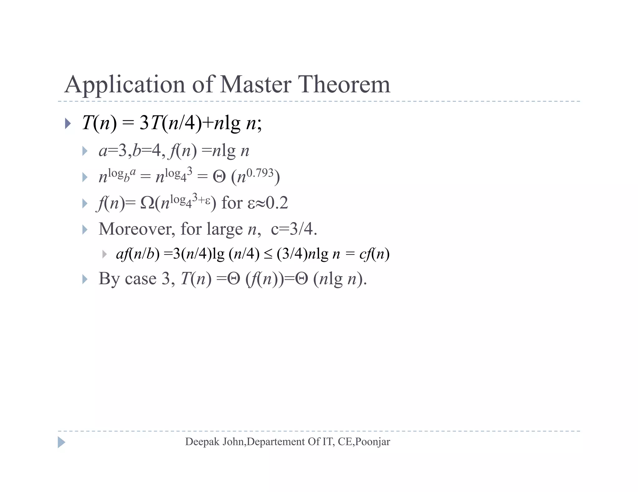
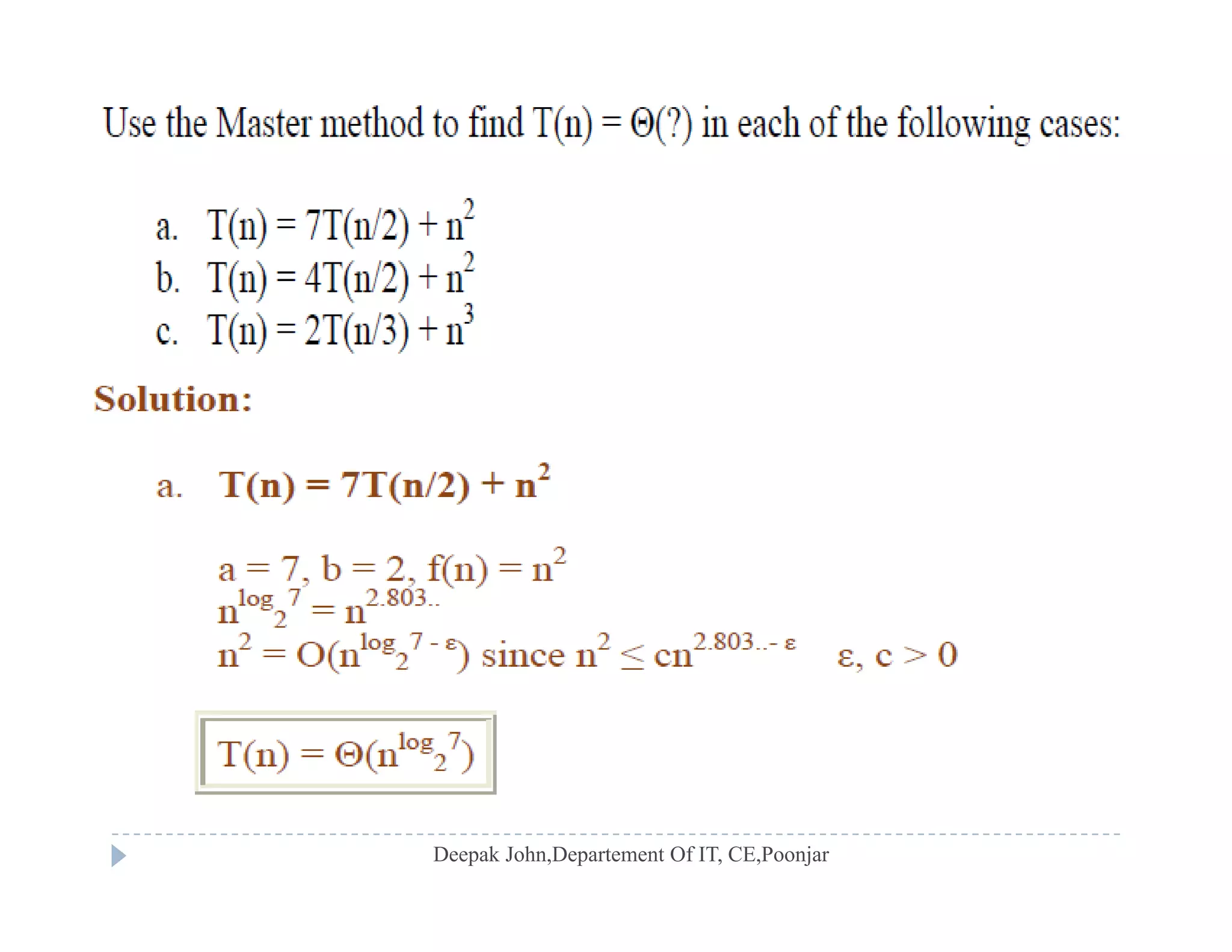
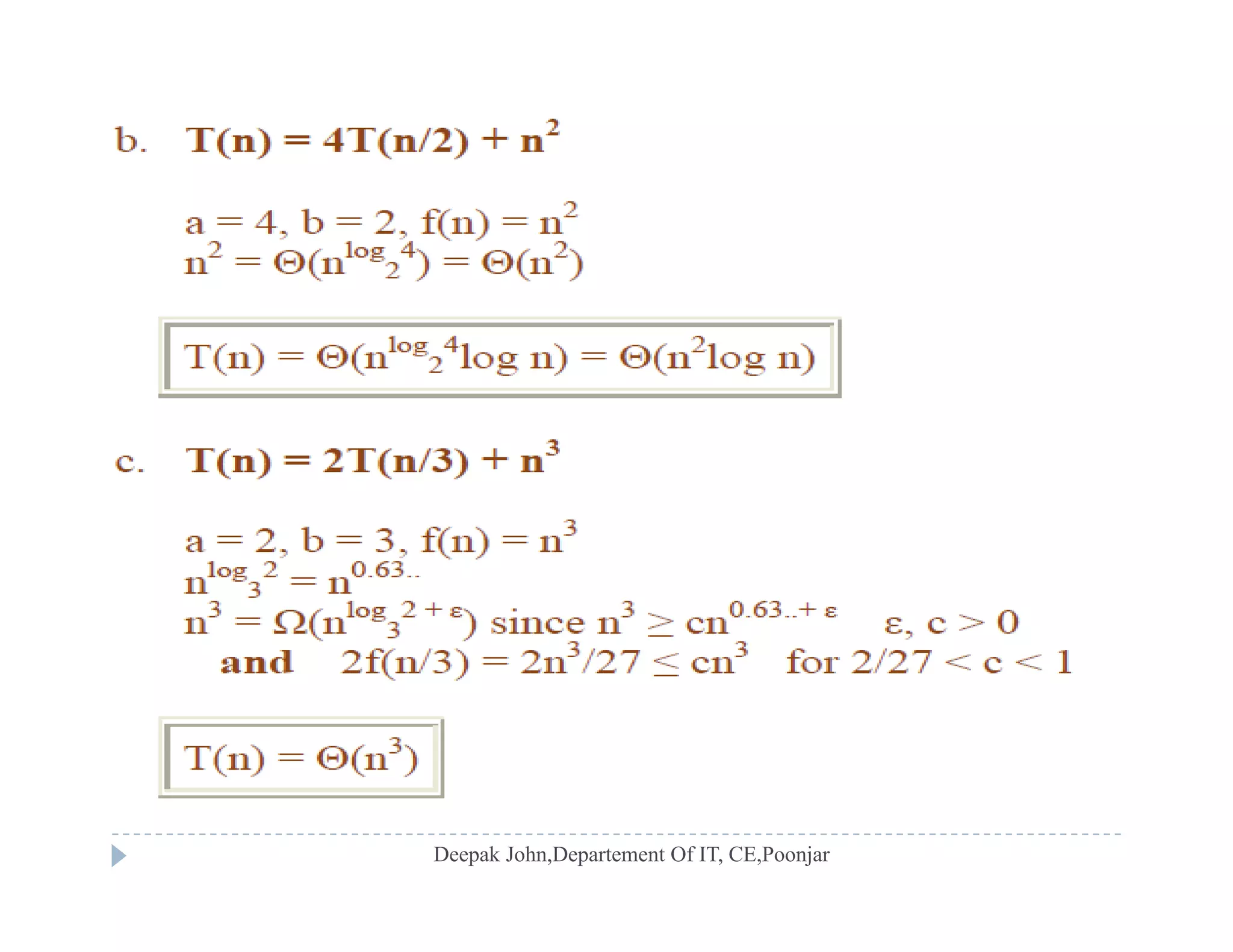
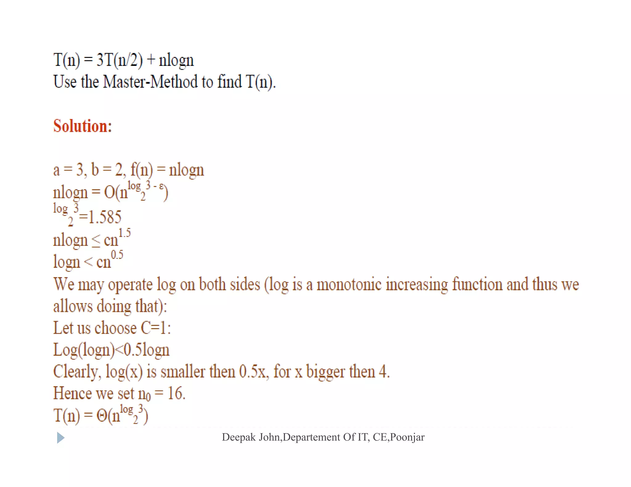
Application of Master Theorem to analyze recurrences, examples provided with different cases.
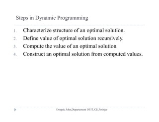
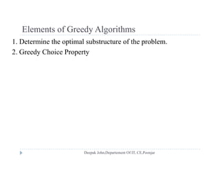
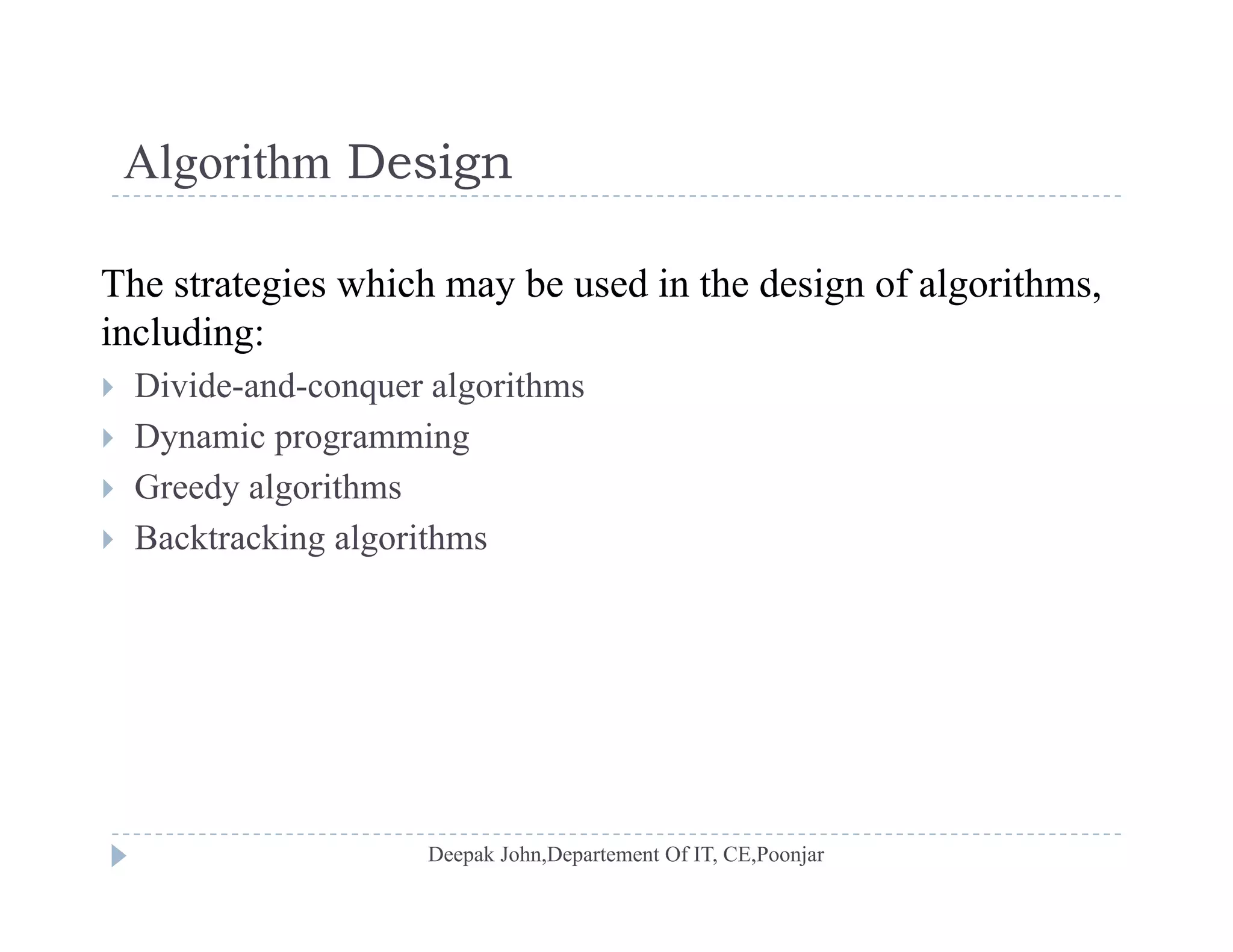
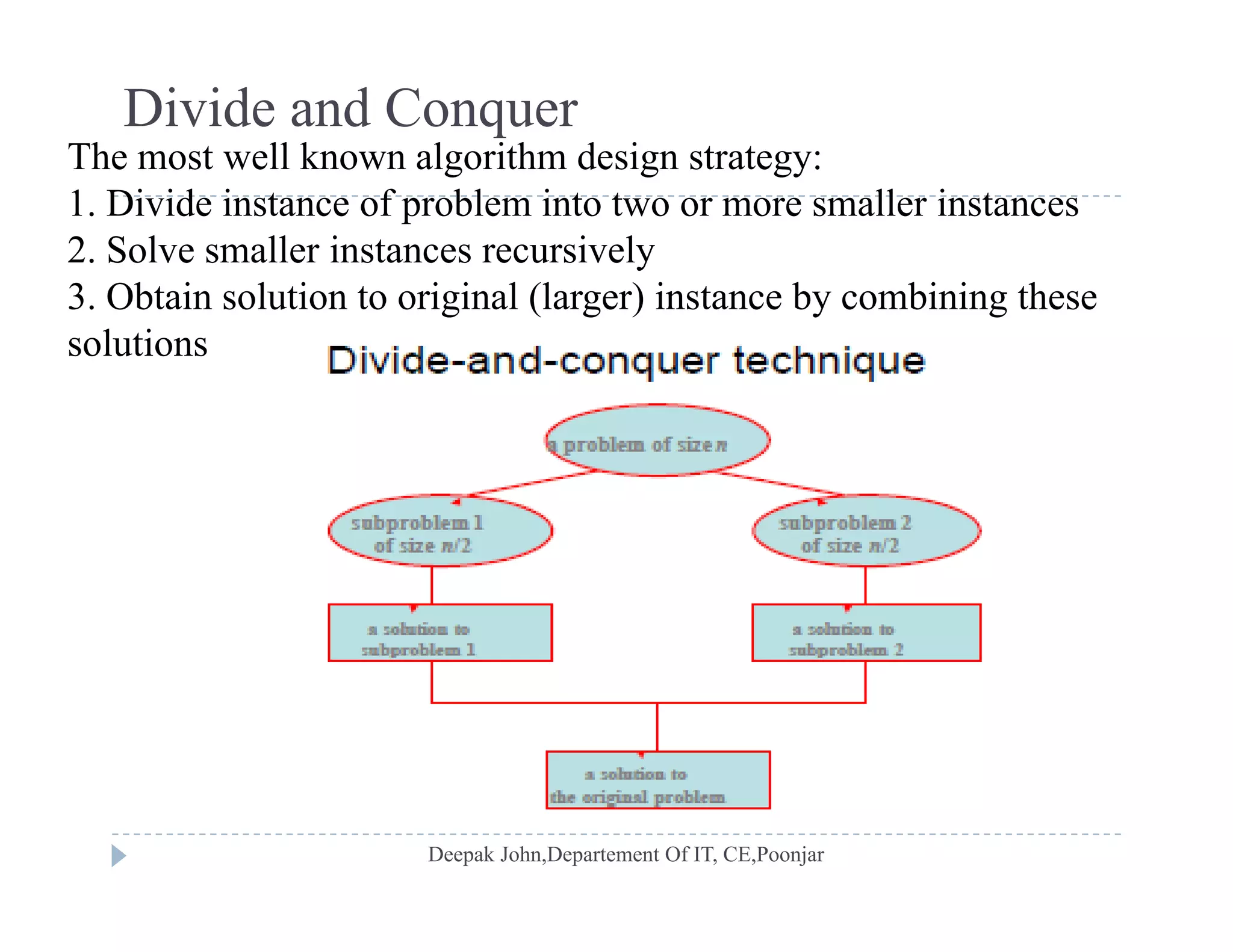
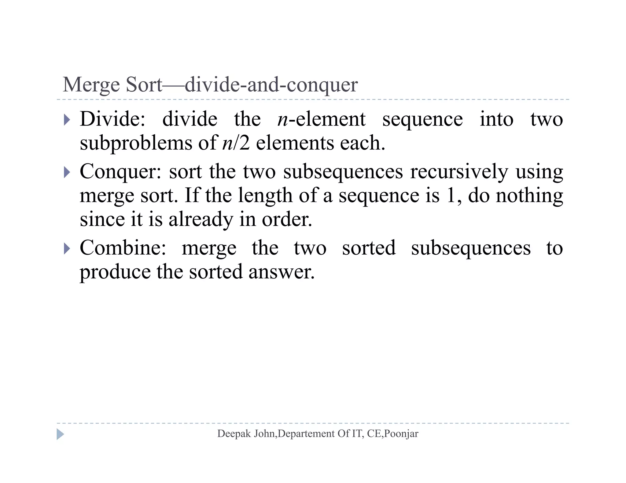
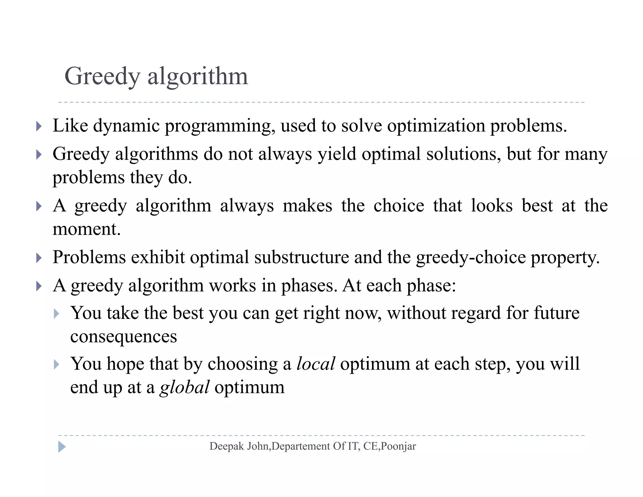
Overview of algorithm design strategies including divide-and-conquer, dynamic programming, and greedy algorithms.
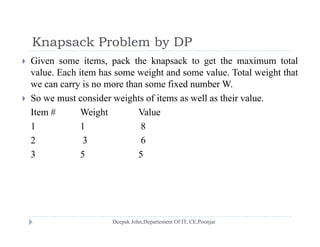
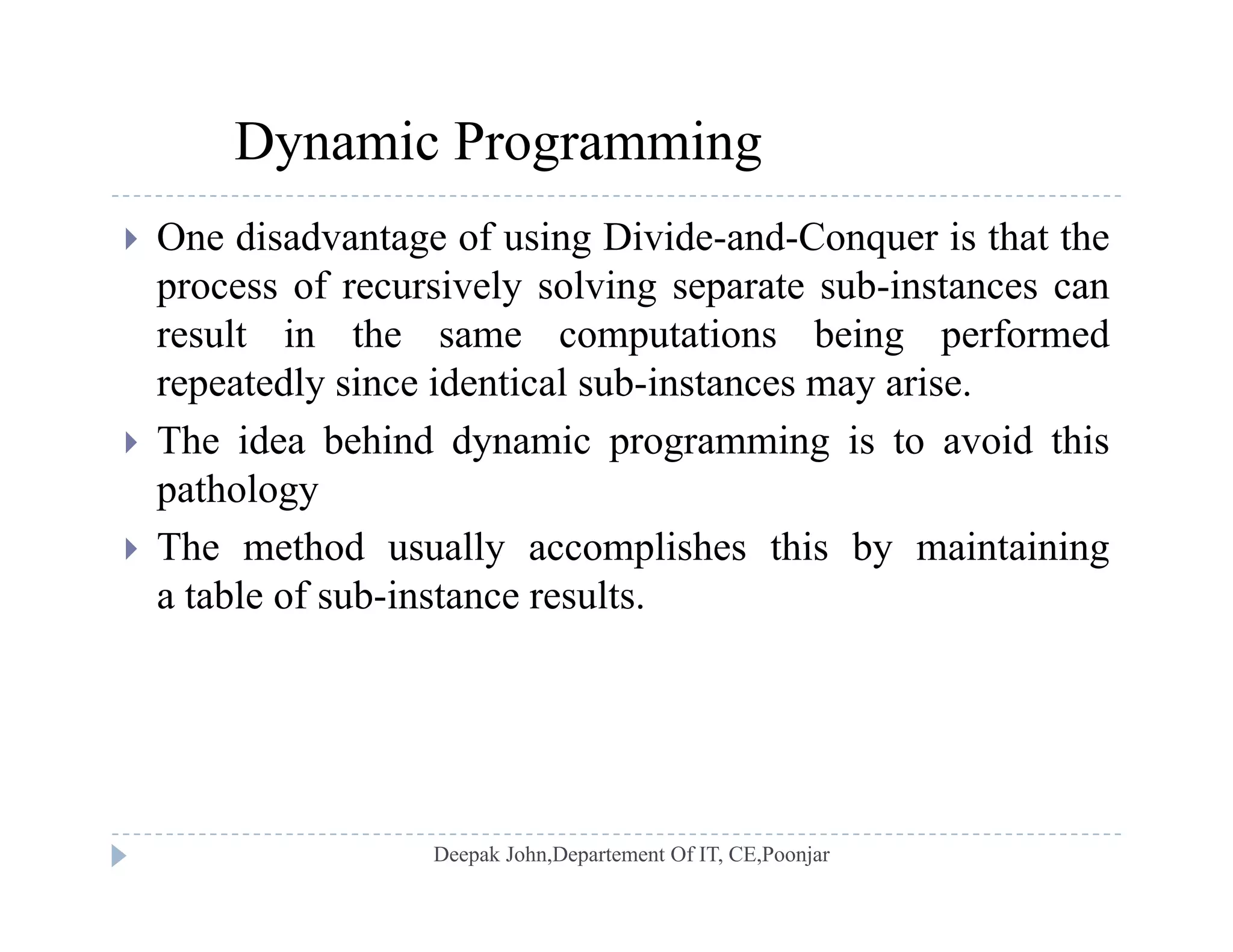
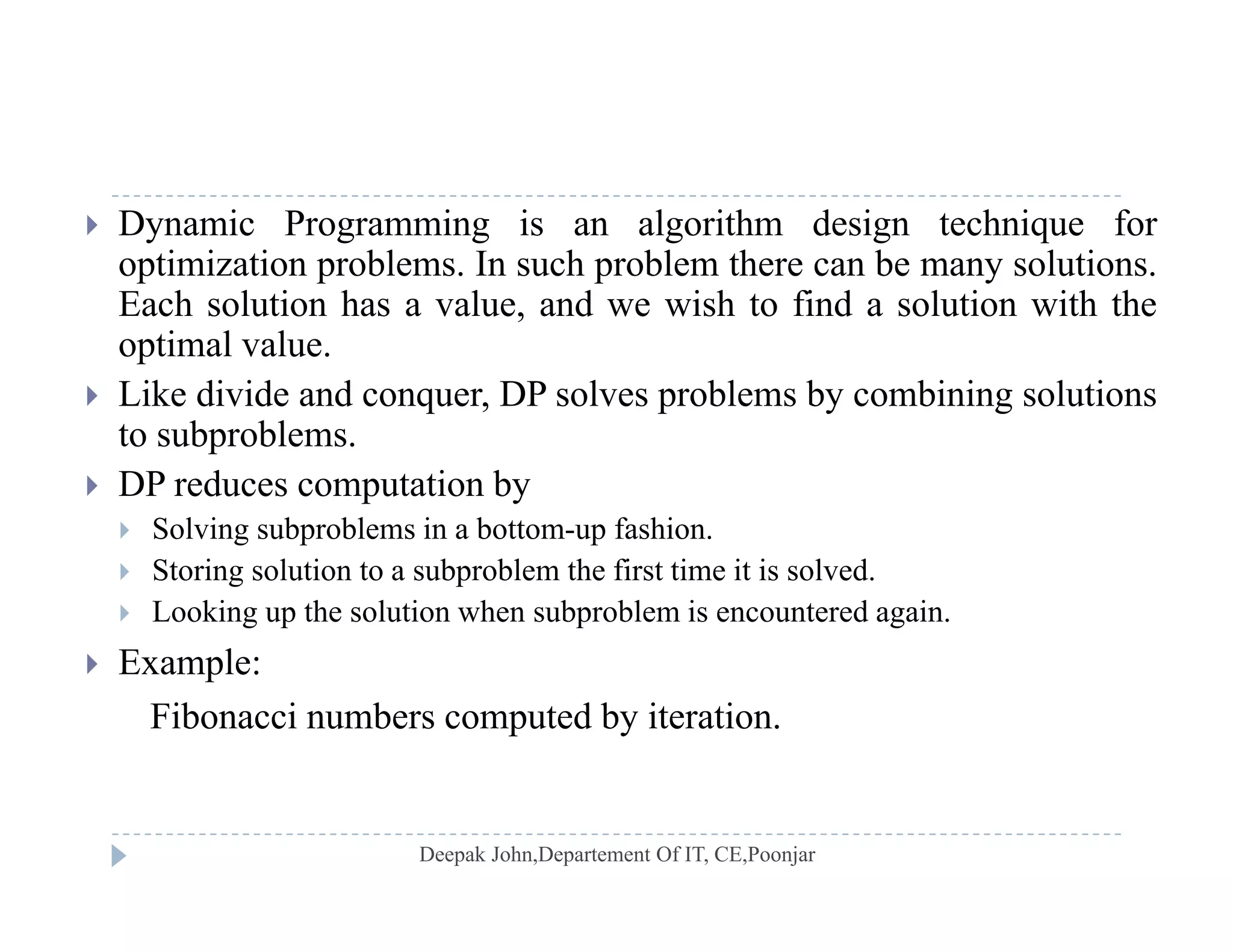
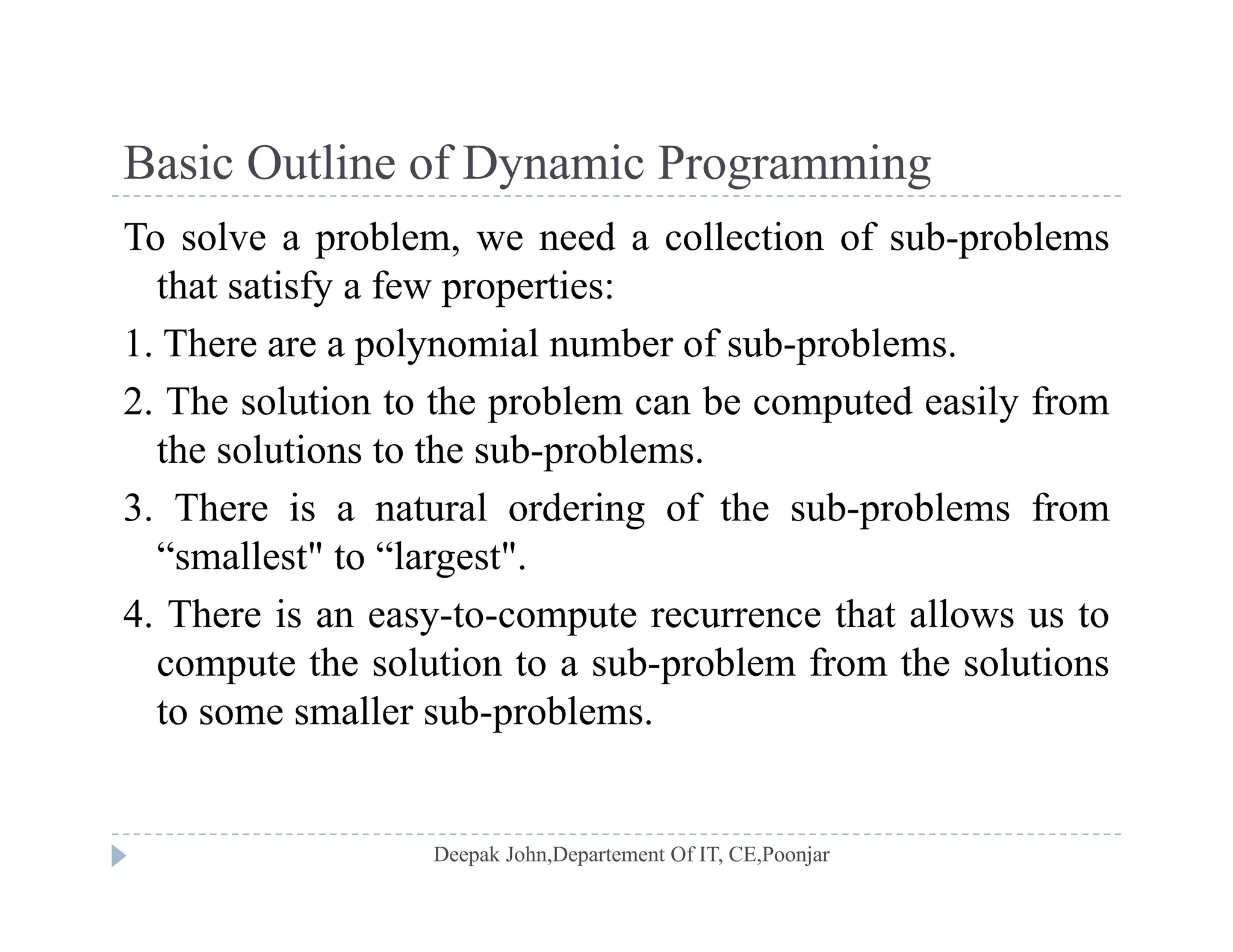
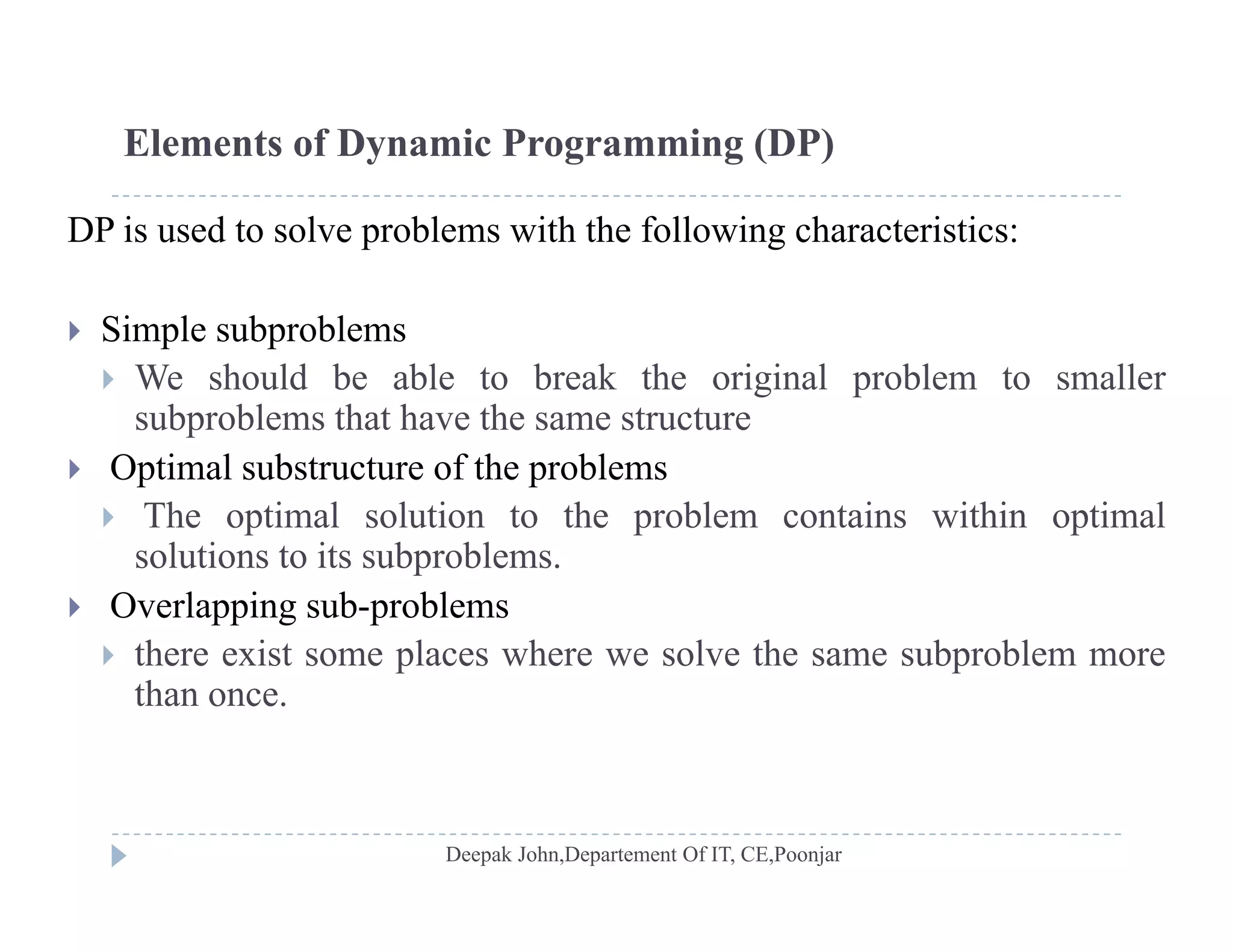
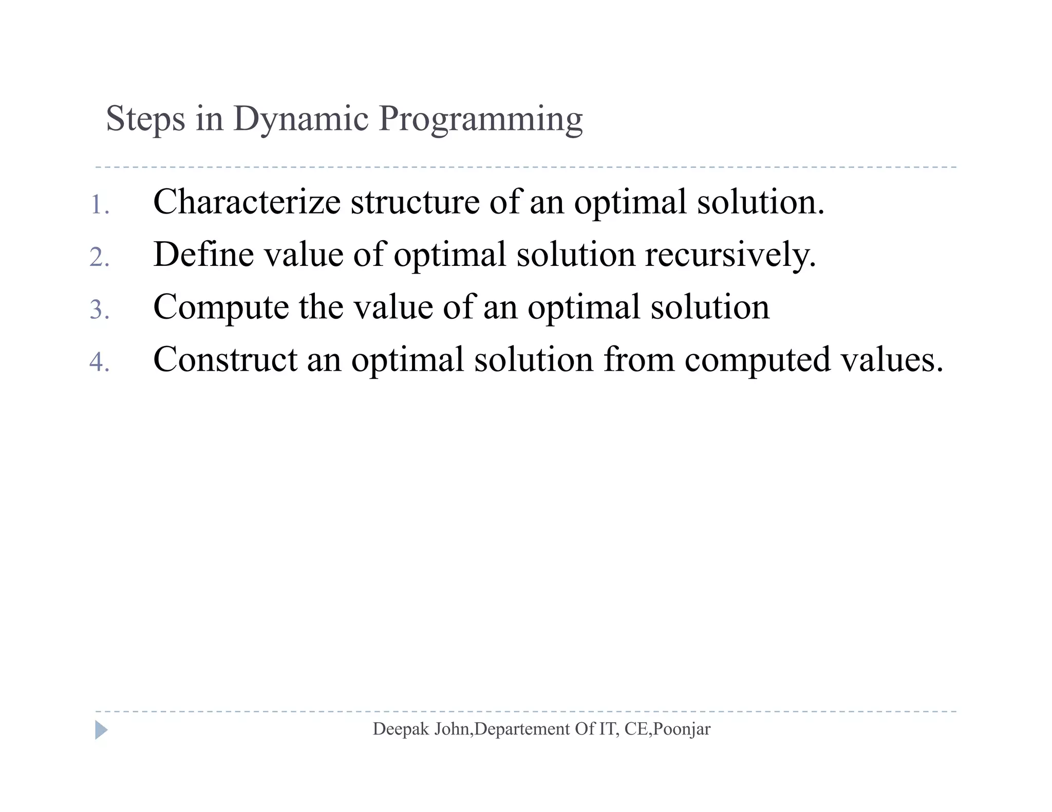
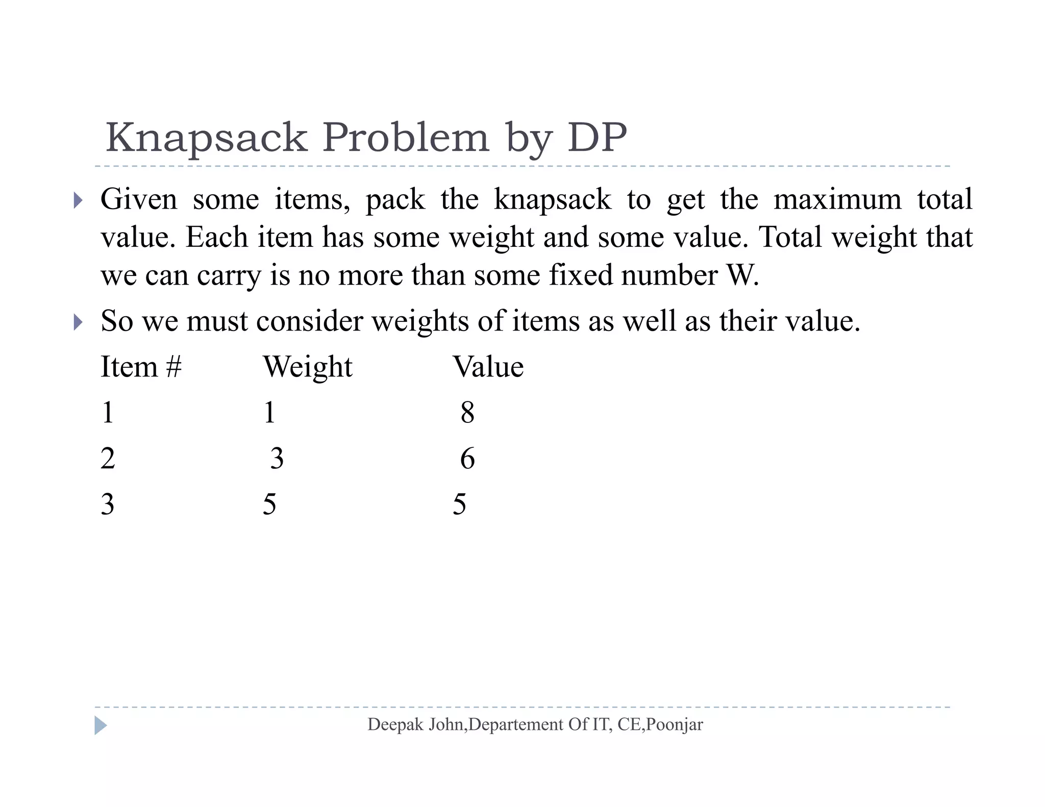
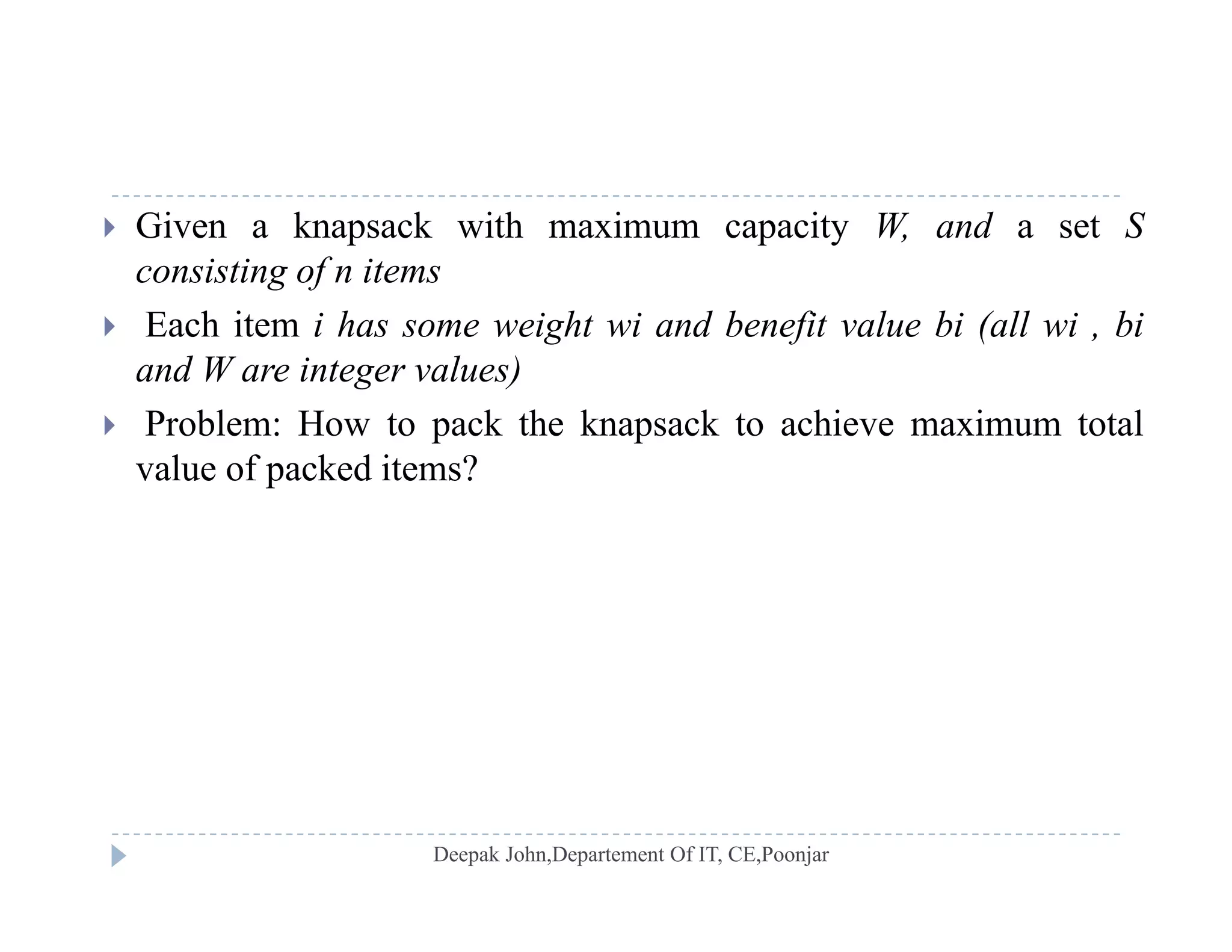
Dynamic programming techniques, their structure, and the knapsack problem as an example.
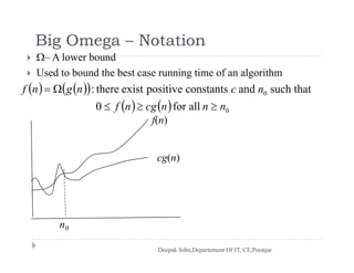
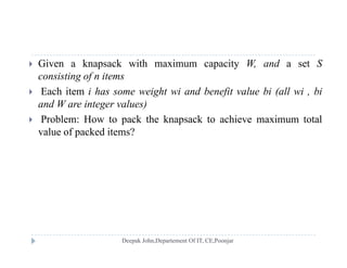
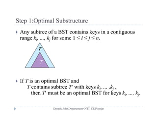
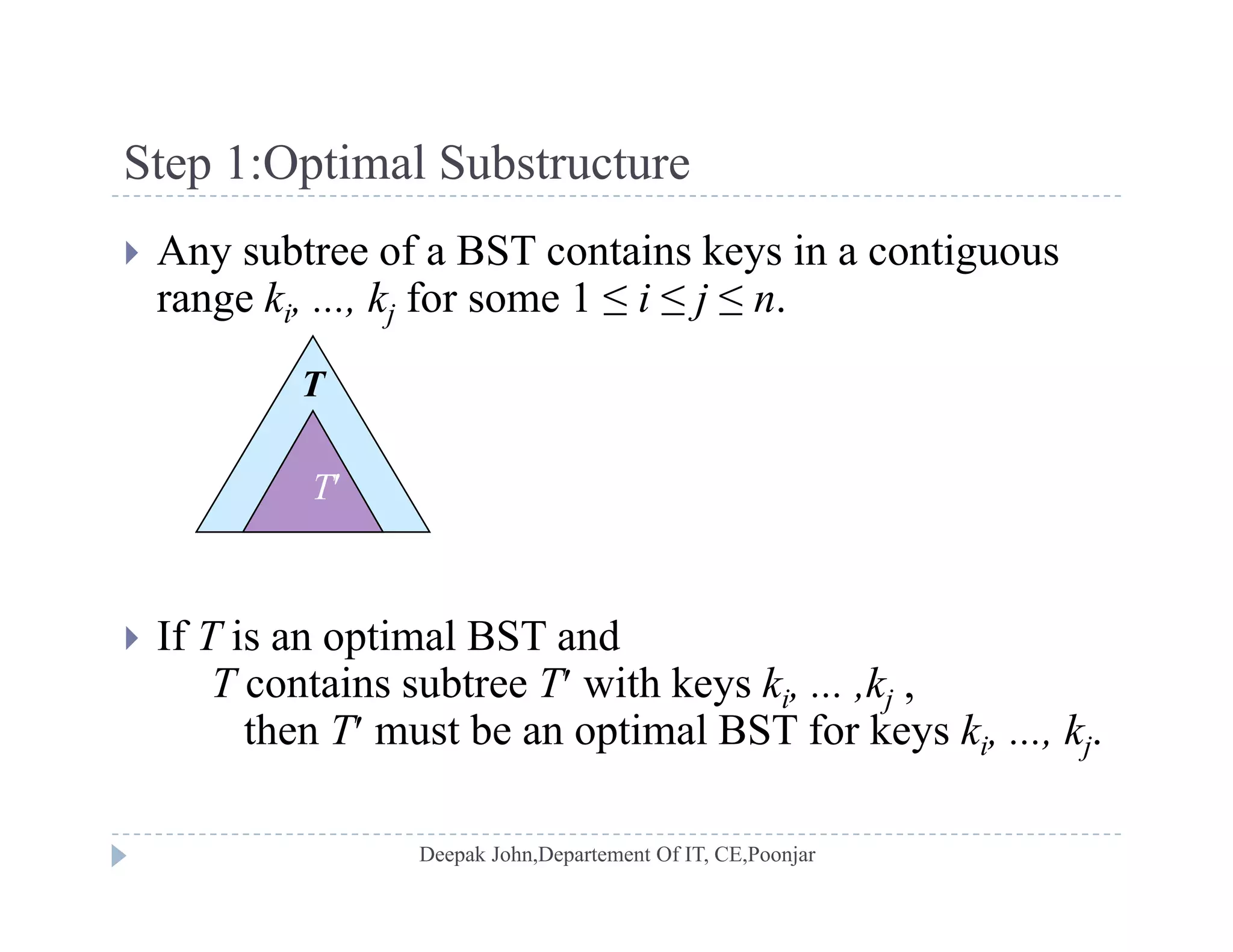
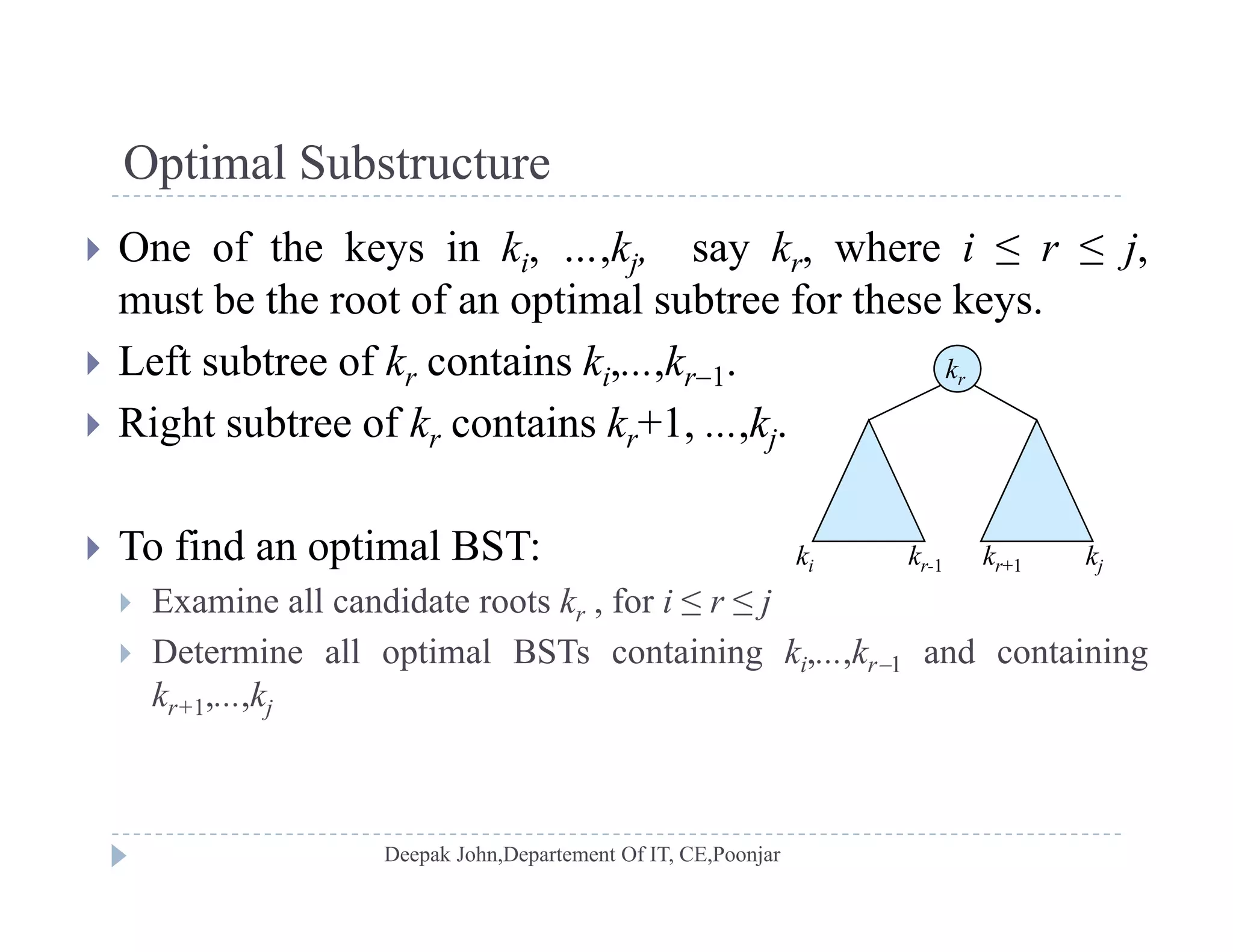
Exploring binary search trees, search costs, and optimal construction strategies.
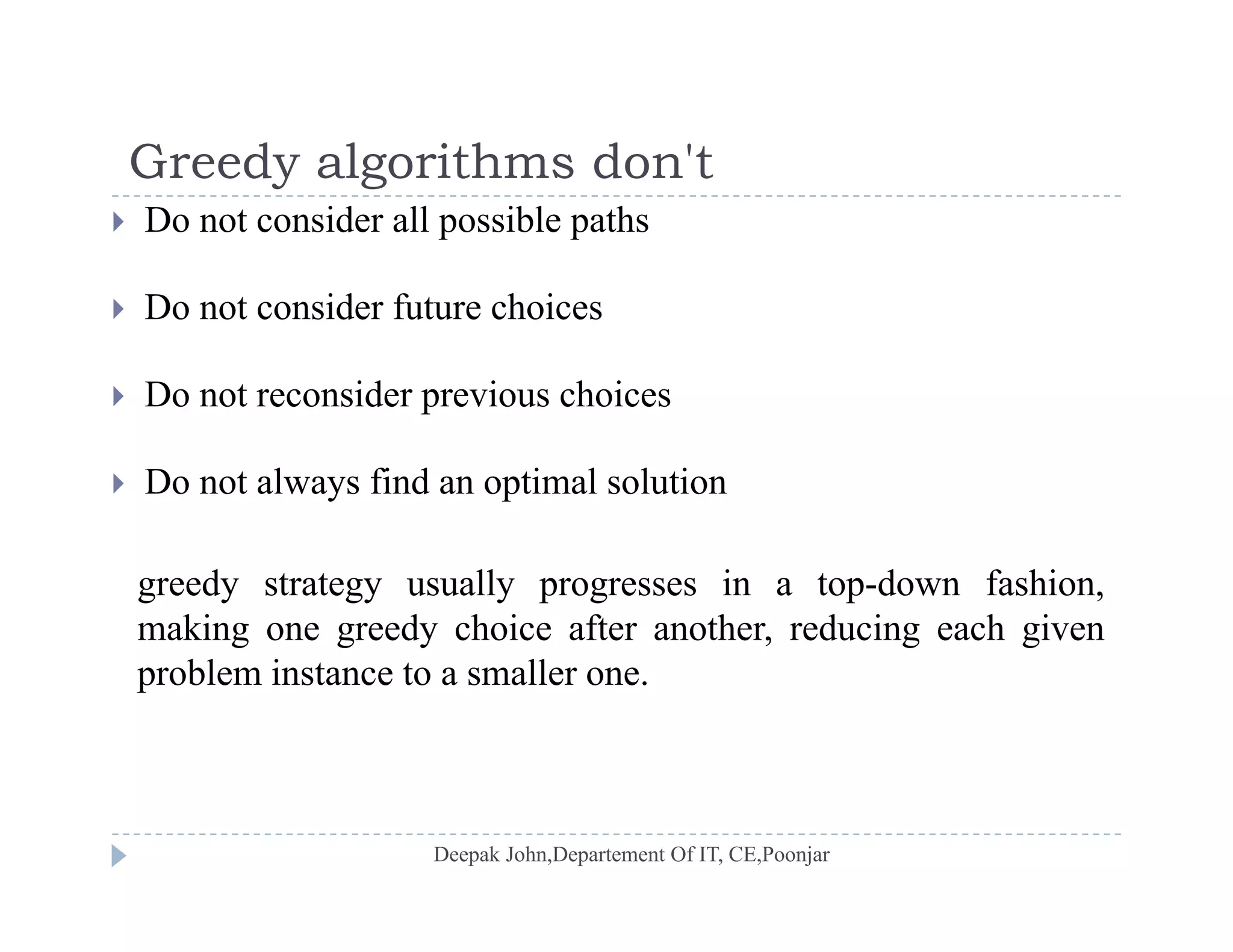
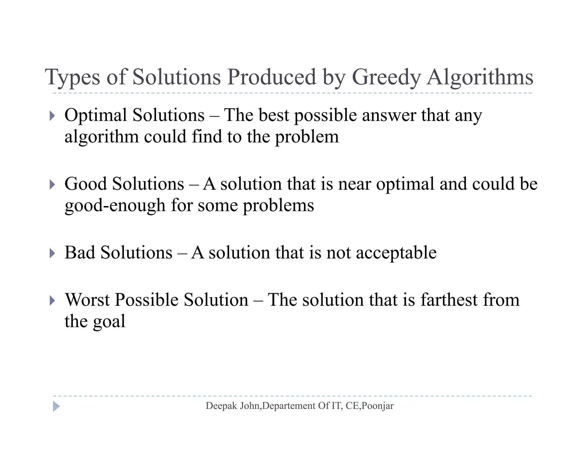
Steps to construct optimal Binary Search Trees: optimal substructure, recursive solutions, and expected cost.Introduction to greedy algorithms, their decision-making process, and the types of solutions they produce.
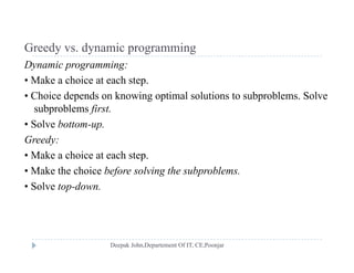
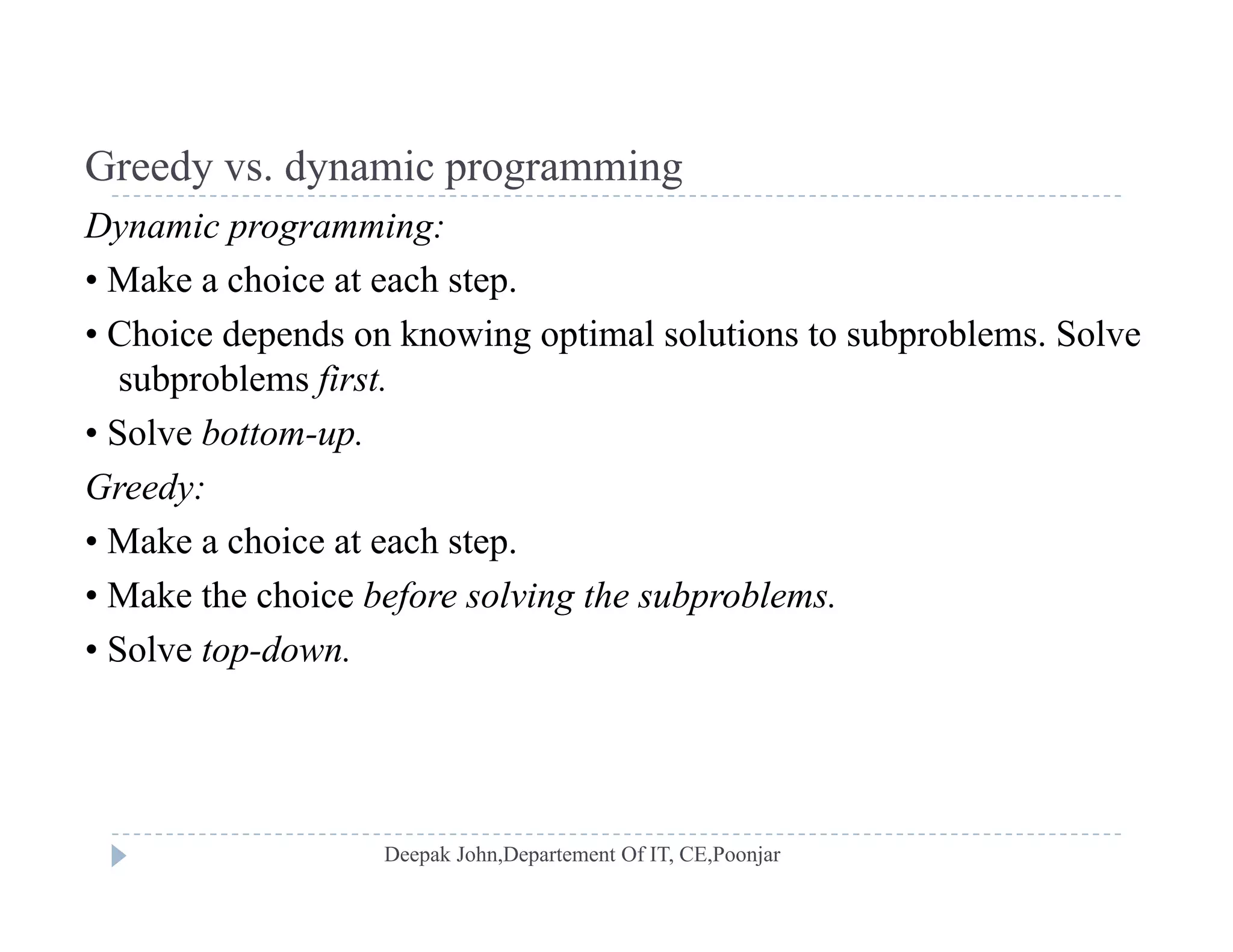
Key differences between greedy algorithms and dynamic programming in problem-solving approaches.
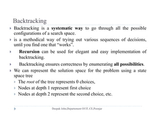
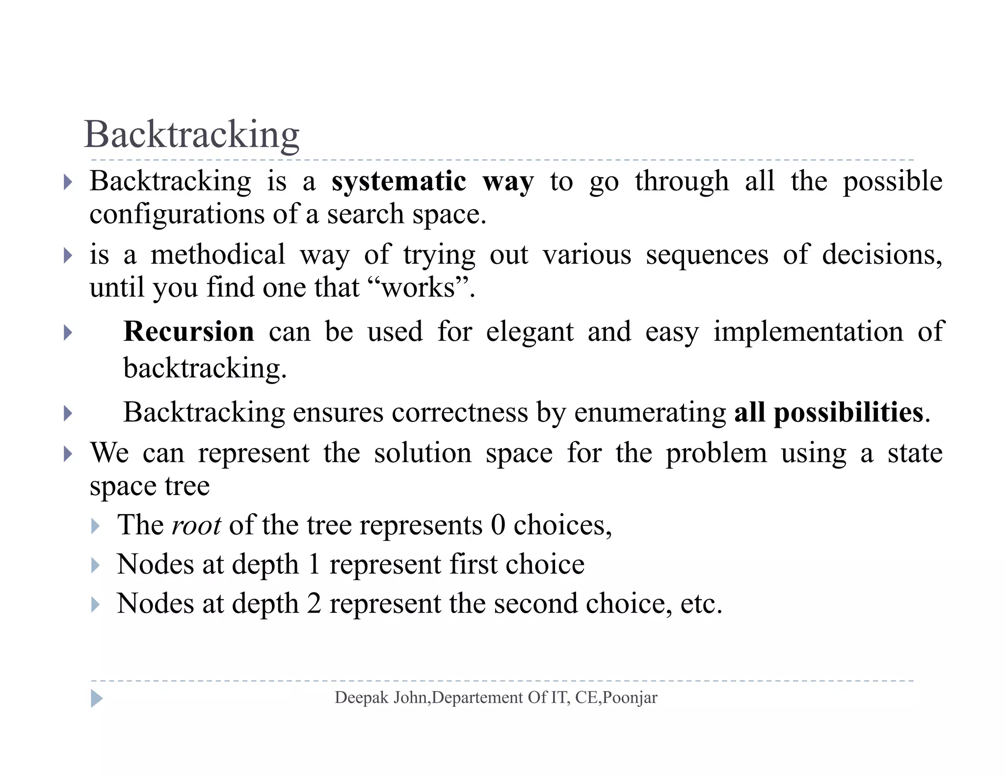
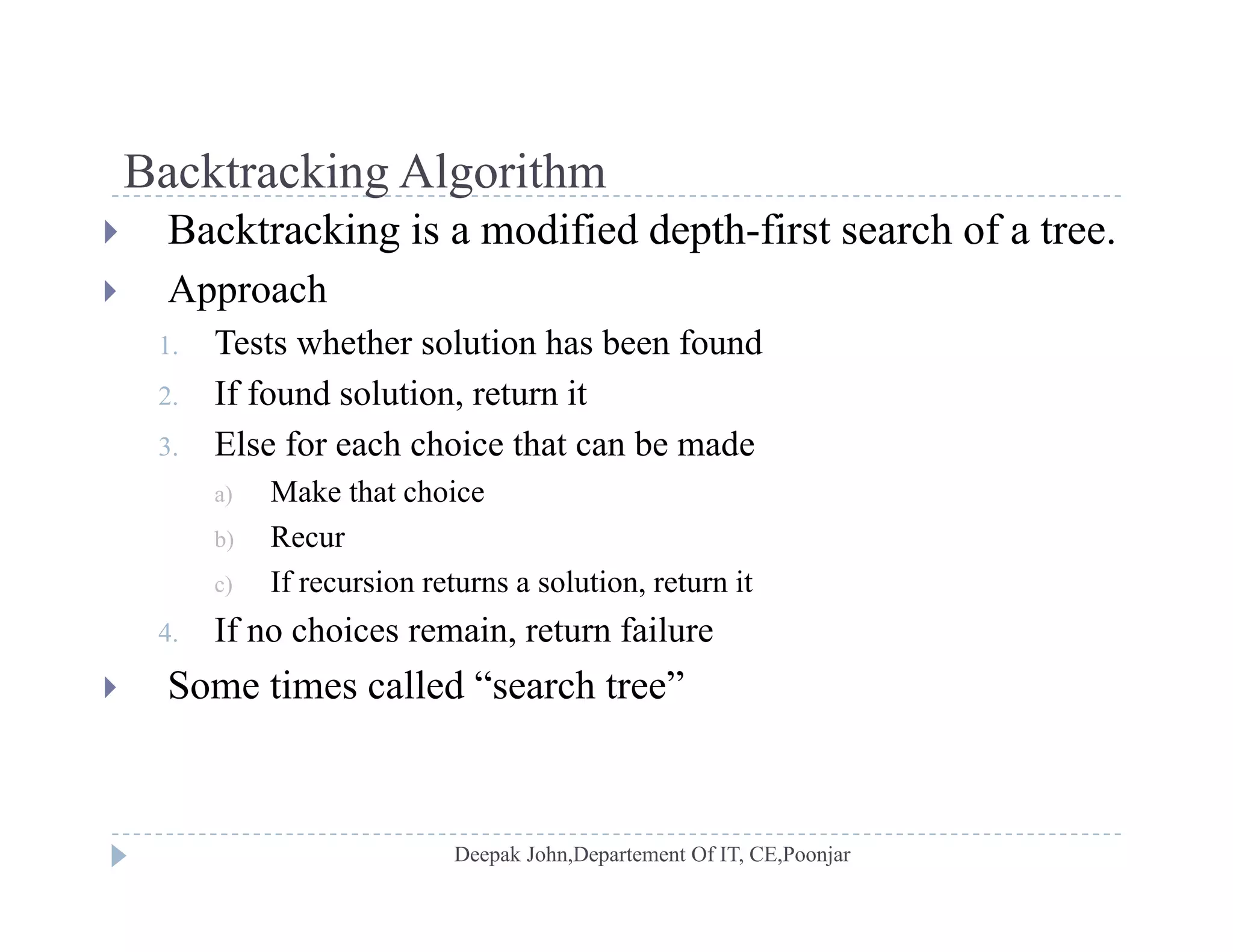
Understanding backtracking as a systematic method for exploring search spaces through recursion.
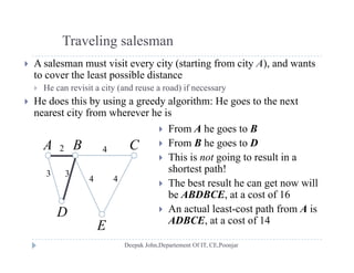
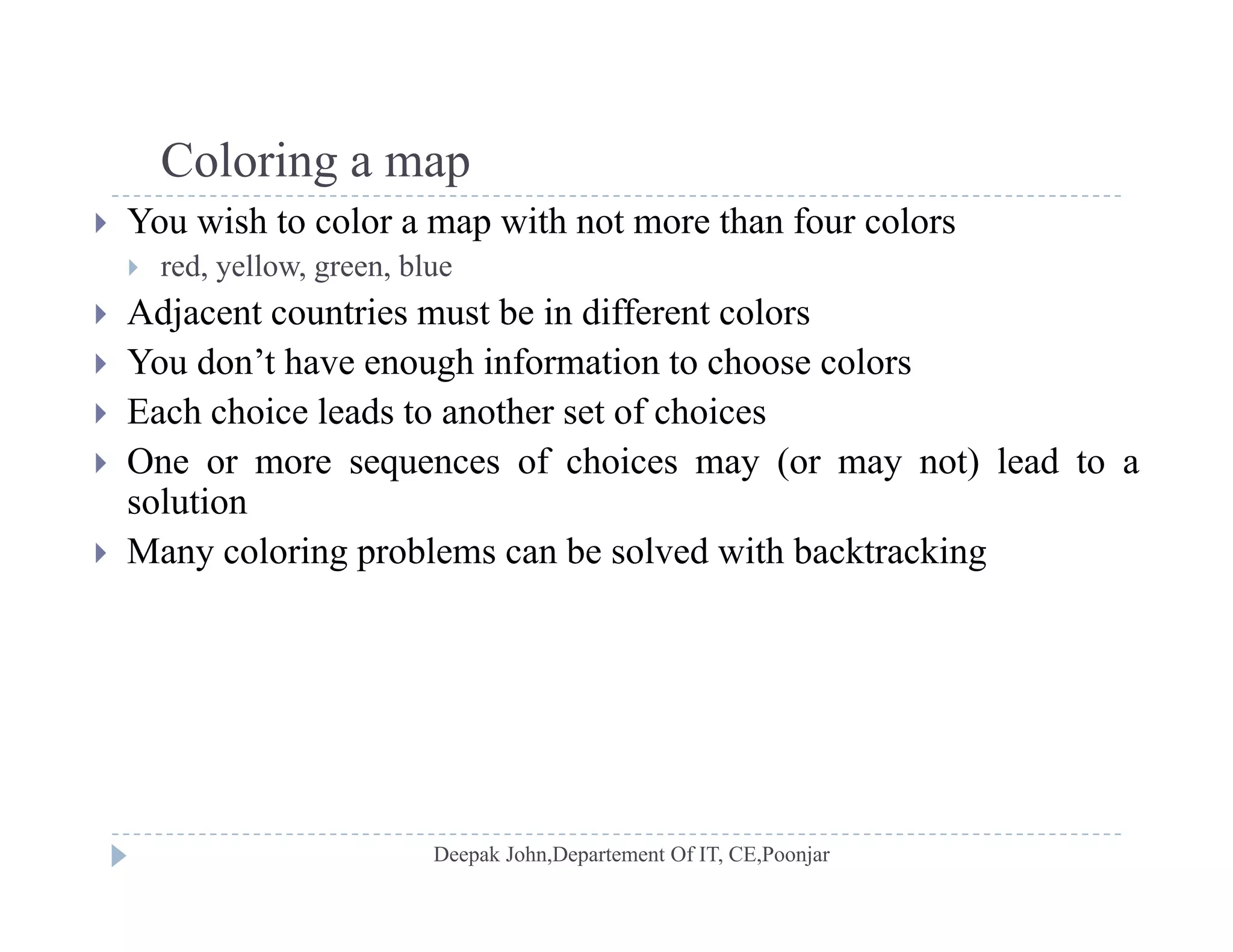
Examples illustrating backtracking, like map coloring, and solving recursion for T(n) equations.


