The document discusses problem-solving agents in artificial intelligence, particularly how they navigate environments to achieve goals through a structured four-phase process: goal formulation, problem formulation, search, and execution. It provides examples of standardized problems such as grid worlds, vacuum environments, and puzzles, outlining their state spaces, initial states, actions, and transition models. Additionally, the text illustrates real-world applications in route-finding and optimization challenges like the traveling salesperson problem and VLSI layout problems.
November 6, 20241
Artificial Intelligence
BCS515B
Module 2
Solving Problems by Searching
2.
November 6, 20242
Solving Problems By Searching
• In which we see how an agent can look ahead to find a sequence of
actions that will eventually achieve its goal.
• When correct action to take is not immediately obvious, an agent
may need to plan ahead: to consider a sequence of actions that
form a path to a goal state. Such an agent is called problem-solving
agent and the computational process it undertakes is called search.
3.
November 6, 20243
Problem Solving Agents
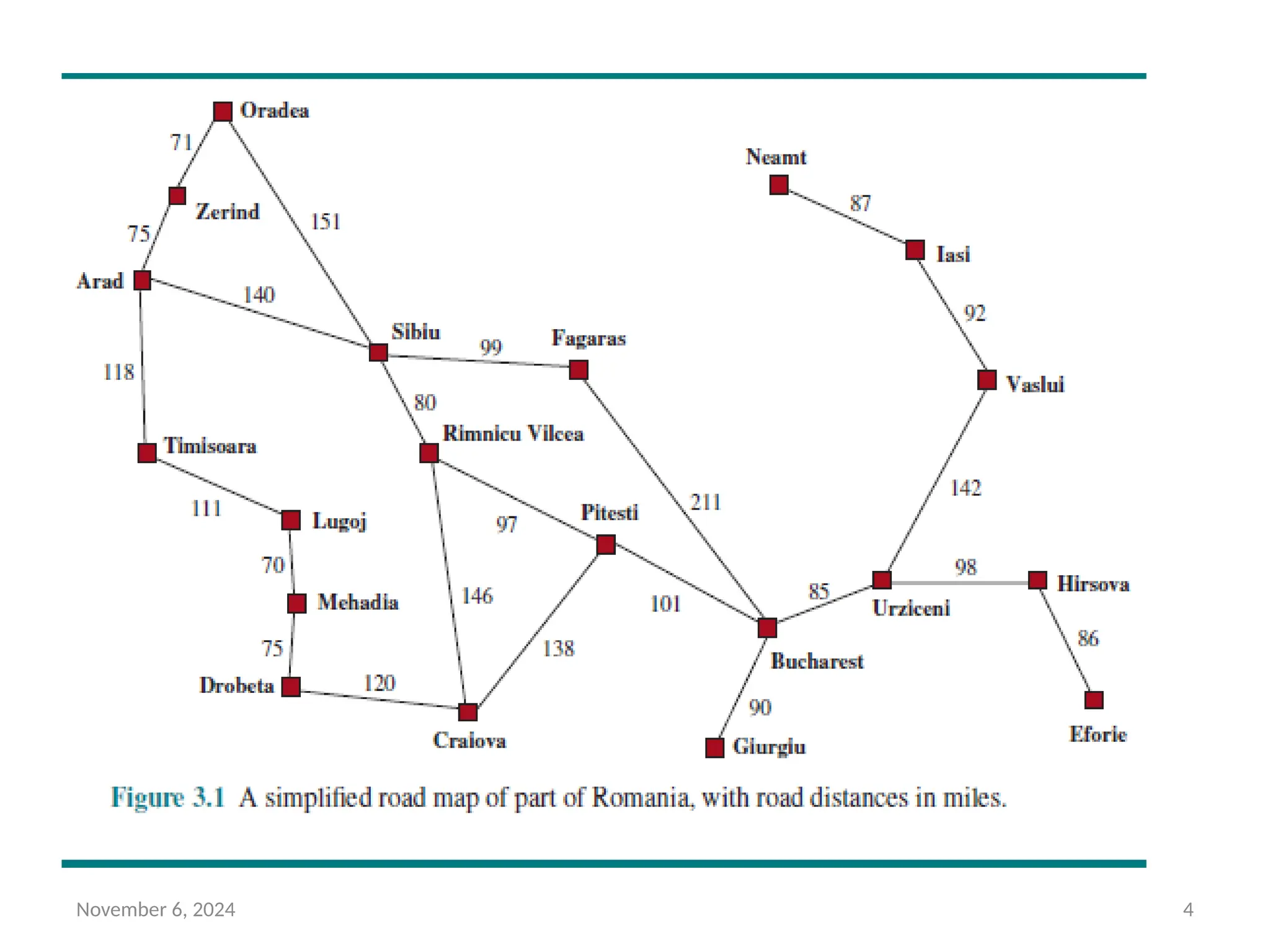
• Imagine an agent enjoying a touring vacation in Romania.
• Suppose agent currently in the city of Arad and has a
nonrefundable ticket to fly out of Bucharest the following day.
• The agent observes street signs and sees that there are three
roads leading out of Arad: one toward Sibiu, one to Timisoara,
and one to Zerind.
• If the agent has no additional information—that is, if the
environment is unknown—then the agent can do no better than
to execute one of the actions at random.
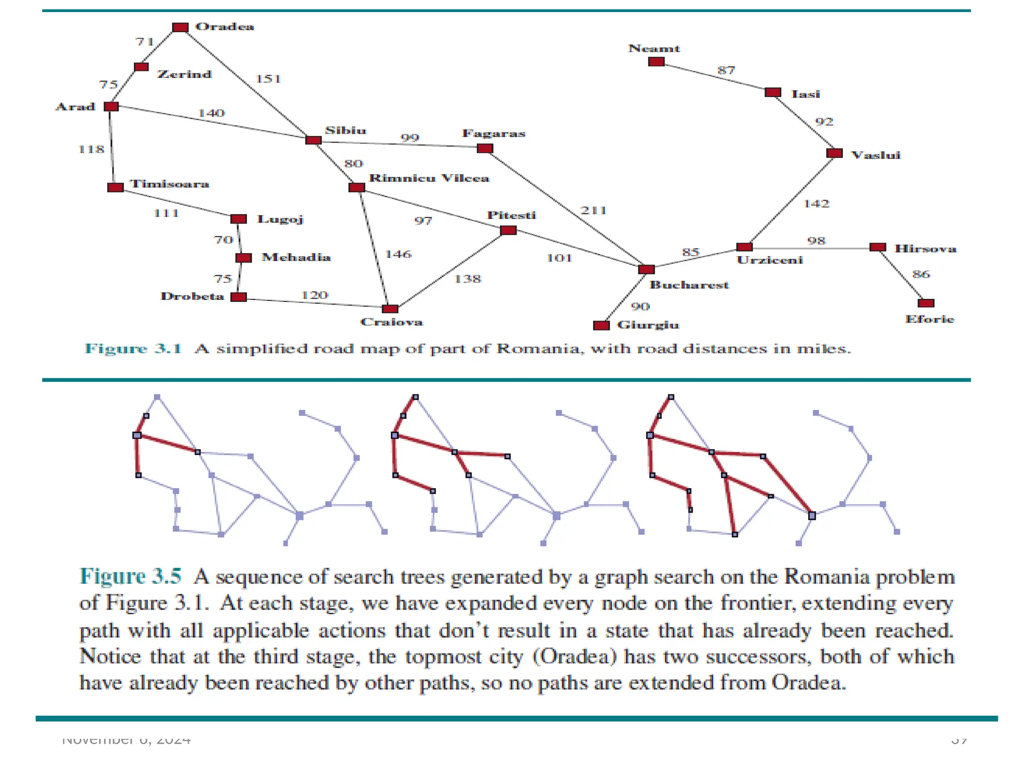
• We assume agent has the information about the world such as a
map in figure 3.1
November 6, 20245
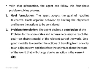
• With that information, the agent can follow this four-phase
problem-solving process:
1. Goal formulation: The agent adopts the goal of reaching
Bucharest. Goals organize behavior by limiting the objectives
and hence the actions to be considered.
2. Problem formulation: The agent devises a description of the
Problem formulation states and actions necessary to reach the
goal—an abstract model of the relevant part of the world. One
good model is to consider the actions of traveling from one city
to an adjacent city, and therefore the only fact about the state
of the world that will change due to an action is the current
city.
6.
November 6, 20246
3. Search: Before taking any action in the real world, the agent
simulates sequences of actions in its model, searching until it
finds a sequence of actions that reaches the goal. Such a
sequence is called a solution. The agent might have to simulate
multiple sequences that do not reach the goal, but eventually
it will find a solution (such as going from Arad to Sibiu to
Fagaras to Bucharest), or it will find that no solution is possible.
4. Execution: The agent can now execute the actions in the
solution, one at a time.
7.
November 6, 20247
• It is an important property that in a fully observable,
deterministic, known environment, the solution to any problem
is a fixed sequence of actions: drive to Sibiu, then Fagaras, then
Bucharest.
• Because the solution is guaranteed to lead to the goal. Control
theorists call this an open-loop system: ignoring the percepts
breaks the loop between agent and environment.
• If there is a chance that the model is incorrect, or the
environment is nondeterministic, then the agent would be safer
using a closed-loop approach that monitors the percepts.
8.
November 6, 20248
Search problems and solutions
A search problem can be defined formally as follows:
• A set of possible states that the environment can be in. We call this the
state space.
• The initial state that the agent starts in. For example: Arad.
• A set of one or more goal states. Sometimes there is one goal state (e.g.,
Bucharest), sometimes there is a small set of alternative goal states, and
sometimes the goal is defined by a property that applies to many states
( infinite), ex: vacuum –cleaner world.
• We can account for all three of these possibilities by specifying an IS-
GOAL method for a problem
9.
November 6, 20249
Search problems and solutions cont….
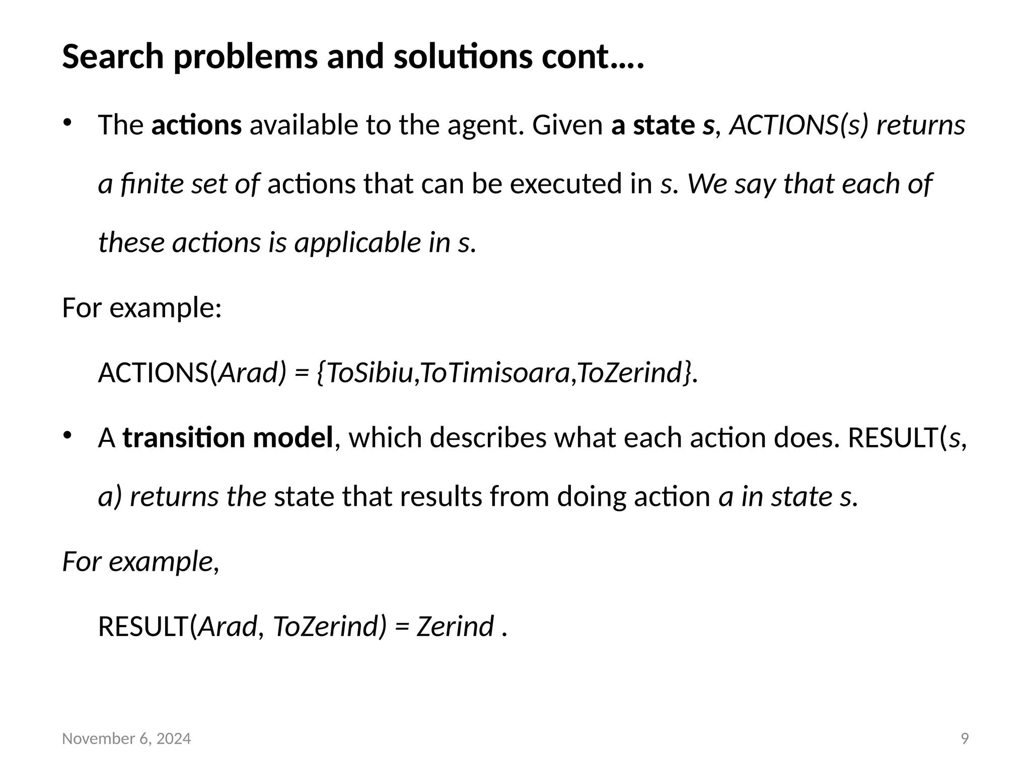
• The actions available to the agent. Given a state s, ACTIONS(s) returns
a finite set of actions that can be executed in s. We say that each of
these actions is applicable in s.
For example:
ACTIONS(Arad) = {ToSibiu,ToTimisoara,ToZerind}.
• A transition model, which describes what each action does. RESULT(s,
a) returns the state that results from doing action a in state s.
For example,
RESULT(Arad, ToZerind) = Zerind .
10.
November 6, 202410
Search problems and solutions cont….
• An action cost function, denoted by ACTION-COST(s,a, s ) when
′
we are programming or c(s,a, s ) when we are doing math, that
′
gives the numeric cost of applying action a in state s to reach
state s .
′
• A problem-solving agent should use a cost function that reflects
its own performance measure; for example, for route-finding
agents, the cost of an action might be the length in miles (as
seen in Figure 3.1), or it might be the time it takes to complete
the action.
11.
November 6, 202411
• A sequence of actions forms a path, and a solution is a path from
the initial state to a goal state.
• We assume that action costs are additive; that is, the total cost of
a path is the sum of the individual action costs.
• An optimal solution has the lowest path cost among all solutions.
• The state space can be represented as a graph in which the
vertices are states and the directed edges between them are
actions.
• The map of Romania shown in Figure 3.1 is such a graph, where
each road indicates two actions, one in each direction.
12.
November 6, 202412
Formulating problems
• Our formulation of the problem of getting to Bucharest is a
model—an abstract mathematical description—and not the real
thing.
• The process of removing detail from a representation is called
abstraction. A good problem formulation has the right level of
detail.
• Level of abstraction: The choice of a good abstraction involves
removing as much detail as possible while retaining validity and
ensuring that the abstract actions are easy to carry out.
Example in our case,
• The action “drive from Arad to Sibiu” can be carried out without
further search or planning by a driver with average skill.
13.
November 6, 202413
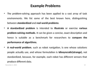
Example Problems
• The problem-solving approach has been applied to a vast array of task
environments. We list some of the best known here, distinguishing
between standardized and real-world problems.
• A standardized problem is intended to illustrate or exercise various
problem-solving methods. It can be given a concise, exact description and
hence is suitable as a benchmark for researchers to compare the
performance of algorithms.
• A real-world problem, such as robot navigation, is one whose solutions
people actually use, and whose formulation is idiosyncratic(strange), not
standardized, because, for example, each robot has different sensors that
produce different data.
14.
November 6, 202414
Standardized problems
A grid world problem
• A grid world problem is a two-dimensional rectangular array
of square cells in which agents can move from cell to cell.
Typically the agent can move to any obstacle-free adjacent
cell—horizontally or vertically and in some problems
diagonally.
• Cells can contain objects, which the agent can pick up, push,
or otherwise act upon; a wall or other impassible obstacle in
a cell prevents an agent from moving into that cell.
November 6, 202416
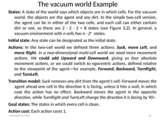
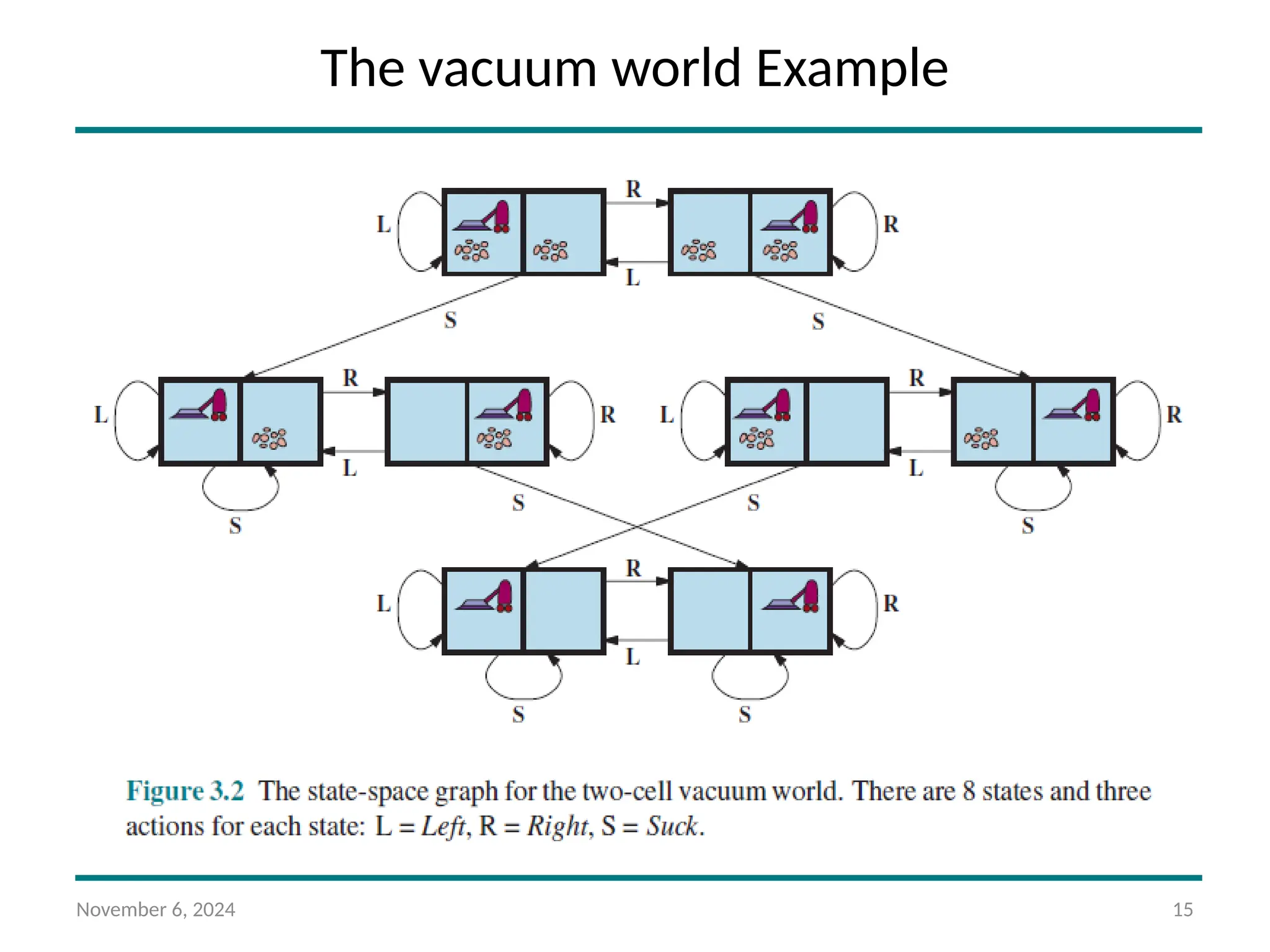
States: A state of the world says which objects are in which cells. For the vacuum
world, the objects are the agent and any dirt. In the simple two-cell version,
the agent can be in either of the two cells, and each call can either contain
dirt or not, so there are 2 · 2 · 2 = 8 states (see Figure 3.2). In general, a
vacuum environment with n cells has n · 2n
states.
Initial state: Any state can be designated as the initial state.
Actions: In the two-cell world we defined three actions: Suck, move Left, and
move Right. In a two-dimensional multi-cell world we need more movement
actions. We could add Upward and Downward, giving us four absolute
movement actions, or we could switch to egocentric actions, defined relative
to the viewpoint of the agent—for example, Forward, Backward, TurnRight,
and TurnLeft.
Transition model: Suck removes any dirt from the agent’s cell; Forward moves the
agent ahead one cell in the direction it is facing, unless it hits a wall, in which
case the action has no effect. Backward moves the agent in the opposite
direction, while TurnRight and TurnLeft change the direction it is facing by 90◦.
Goal states: The states in which every cell is clean.
Action cost: Each action costs 1.
The vacuum world Example
17.
November 6, 202417
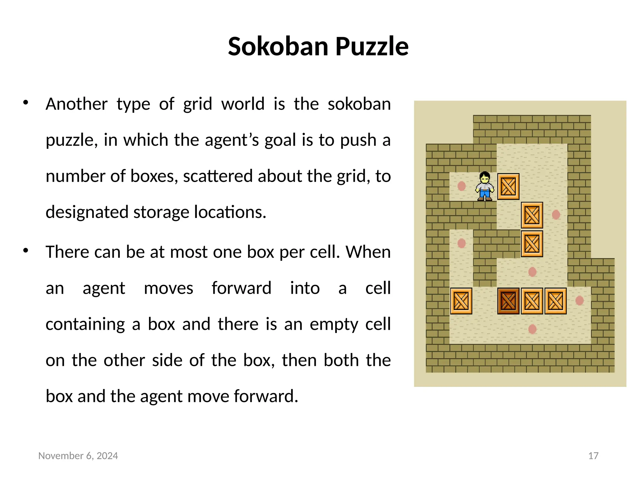
Sokoban Puzzle
• Another type of grid world is the sokoban
puzzle, in which the agent’s goal is to push a
number of boxes, scattered about the grid, to
designated storage locations.
• There can be at most one box per cell. When
an agent moves forward into a cell
containing a box and there is an empty cell
on the other side of the box, then both the
box and the agent move forward.
18.
November 6, 202418
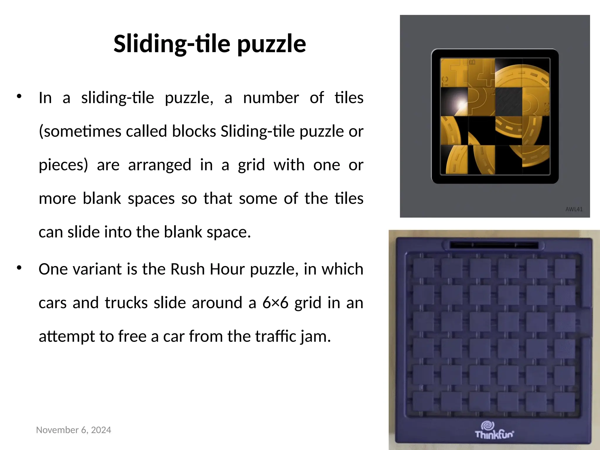
Sliding-tile puzzle
• In a sliding-tile puzzle, a number of tiles
(sometimes called blocks Sliding-tile puzzle or
pieces) are arranged in a grid with one or
more blank spaces so that some of the tiles
can slide into the blank space.
• One variant is the Rush Hour puzzle, in which
cars and trucks slide around a 6×6 grid in an
attempt to free a car from the traffic jam.
19.
November 6, 202419
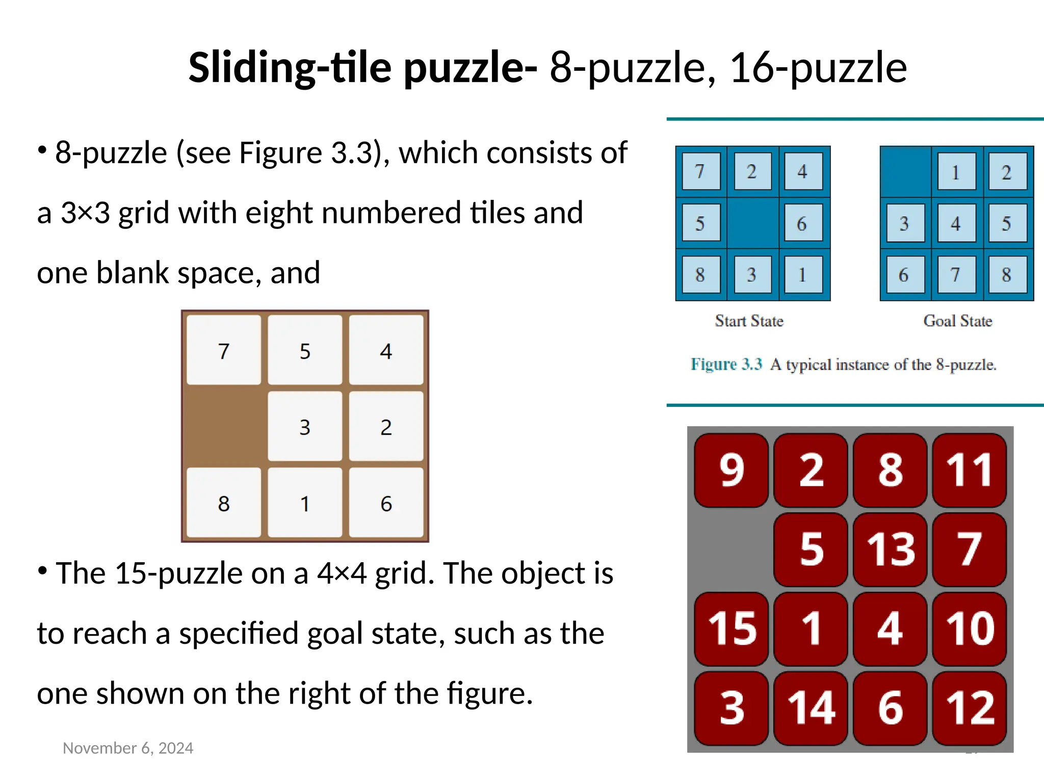
Sliding-tile puzzle- 8-puzzle, 16-puzzle
• 8-puzzle (see Figure 3.3), which consists of
a 3×3 grid with eight numbered tiles and
one blank space, and
• The 15-puzzle on a 4×4 grid. The object is
to reach a specified goal state, such as the
one shown on the right of the figure.
20.
November 6, 202420
The standard formulation of the 8 puzzle is as follows:
• States: A state description specifies the location of each of the tiles.
• Initial state: Any state can be designated as the initial state.
• Actions: While in the physical world it is a tile that slides, the simplest way
of describing an action is to think of the blank space moving Left, Right,
Up, or Down. If the blank is at an edge or corner then not all actions will be
applicable.
• Transition model: Maps a state and action to a resulting state; for example,
if we apply Left to the start state in Figure 3.3, the resulting state has the 5
and the blank switched.
• Goal state: Although any state could be the goal, we typically specify a
state with the numbers in order, as in Figure 3.3.
• Action cost: Each action costs 1.
21.
November 6, 202421
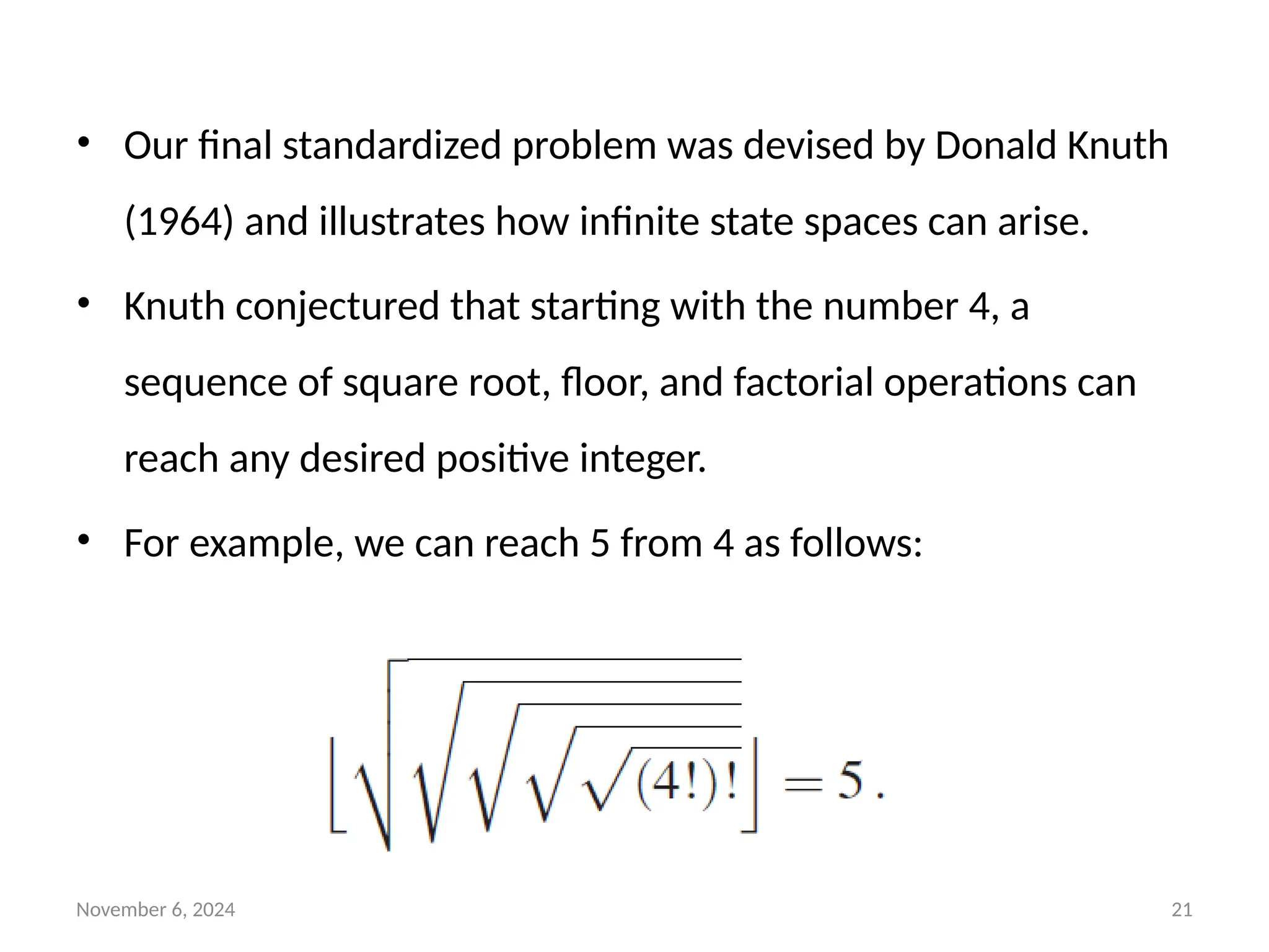
• Our final standardized problem was devised by Donald Knuth
(1964) and illustrates how infinite state spaces can arise.
• Knuth conjectured that starting with the number 4, a
sequence of square root, floor, and factorial operations can
reach any desired positive integer.
• For example, we can reach 5 from 4 as follows:
22.
November 6, 202422
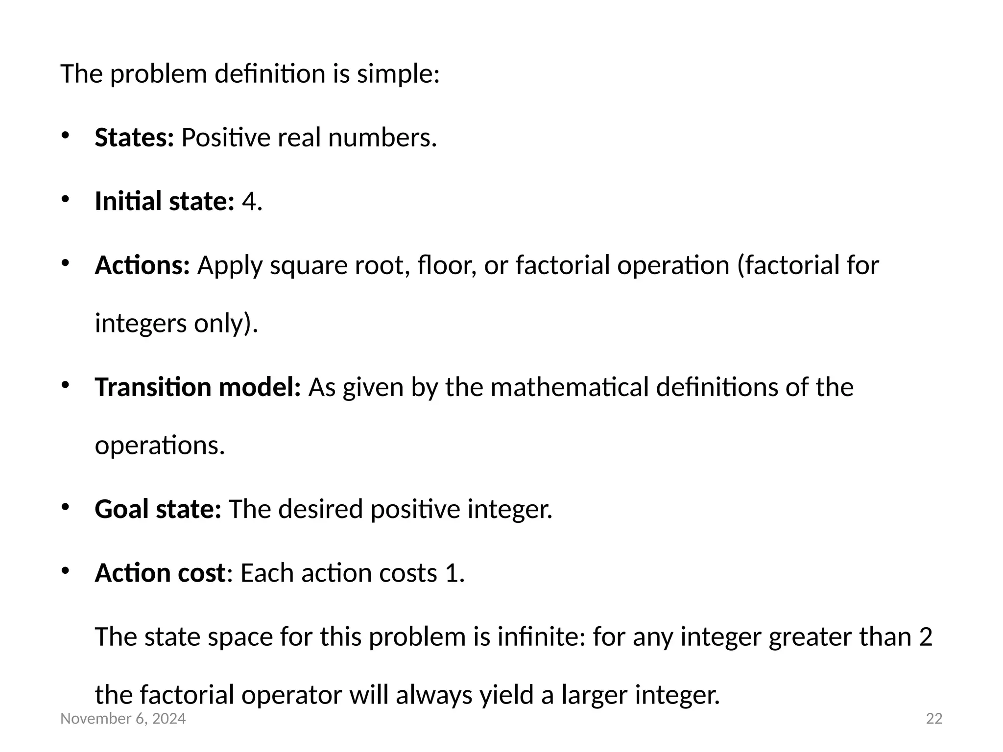
The problem definition is simple:
• States: Positive real numbers.
• Initial state: 4.
• Actions: Apply square root, floor, or factorial operation (factorial for
integers only).
• Transition model: As given by the mathematical definitions of the
operations.
• Goal state: The desired positive integer.
• Action cost: Each action costs 1.
The state space for this problem is infinite: for any integer greater than 2
the factorial operator will always yield a larger integer.
23.
November 6, 202423
8-queens problem
• The goal of the 8-queens problem is to place eight queens on
a chessboard such that no queen attacks any other. (A queen
attacks any piece in the same row, column or diagonal.)
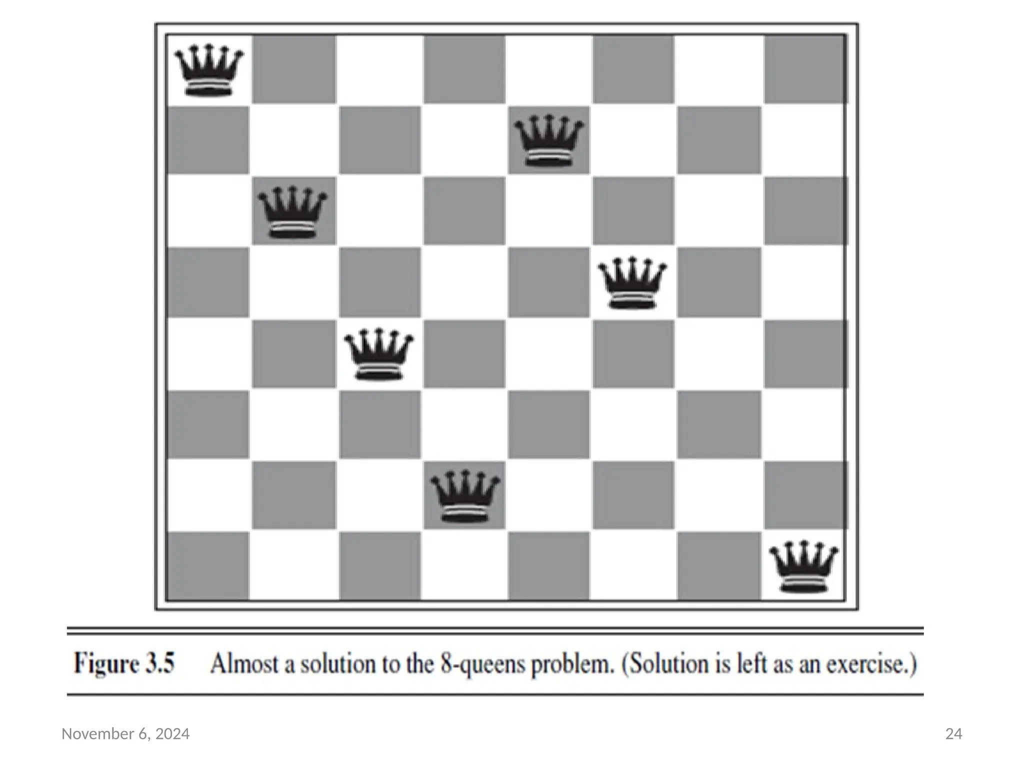
• Figure 3.5 shows an attempted solution that fails: the queen
in the rightmost column is attacked by the queen at the top
left.
November 6, 202425
• There are two main kinds of formulation.
1. incremental formulation
2. complete-state formulation
• An incremental formulation involves operators that augment the
state description, starting with an empty state; for the 8-queens
problem, this means that each action adds a queen to the state.
• A complete-state formulation starts with all 8 queens on the
board and moves them around
26.
November 6, 202426
• The first incremental formulation one might try is the
following:
• States: Any arrangement of 0 to 8 queens on the board is a
state.
• Initial state: No queens on the board.
• Actions: Add a queen to any empty square.
• Transition model: Returns the board with a queen added to
the specified square.
• Goal test: 8 queens are on the board, none attacked.
• In this formulation, we have 64 ・ 63 ・ ・ ・ 57 ≈
1.8×10¹⁴
possible sequences to investigate.
27.
November 6, 202427
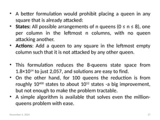
• A better formulation would prohibit placing a queen in any
square that is already attacked:
• States: All possible arrangements of n queens (0 ≤ n ≤ 8), one
per column in the leftmost n columns, with no queen
attacking another.
• Actions: Add a queen to any square in the leftmost empty
column such that it is not attacked by any other queen.
• This formulation reduces the 8-queens state space from
1.8×10¹⁴
to just 2,057, and solutions are easy to find.
• On the other hand, for 100 queens the reduction is from
roughly 10400
states to about 1052
states -a big improvement,
but not enough to make the problem tractable.
• A simple algorithm is available that solves even the million-
queens problem with ease.
November 6, 202429
Real-world problems
• We have already seen how the route-finding
problem is defined in terms of specified
locations and transitions along edges between
them.
• Route-finding algorithms are used in a variety
of applications. Some, such as Web sites and
in-car systems that provide driving directions,
are relatively straightforward extensions of the
Romania example.
• (The main complications are varying costs
due to traffic-dependent delays, and
rerouting due to road closures.)
• Others, such as routing video streams in
computer networks, military operations
planning, and airline travel-planning systems,
involve much more complex specifications.
30.
November 6, 202430
Consider the airline travel problems that must be solved by a travel-planning
Web site:
• States: Each state obviously includes a location (e.g., an airport) and the
current time. Furthermore, because the cost of an action (a flight segment)
may depend on previous segments, their fare bases, and their status as
domestic or international, the state must record extra information about
these “historical” aspects.
• Initial state: The user’s home airport.
• Actions: Take any flight from the current location, in any seat class, leaving
after the current time, leaving enough time for within-airport transfer if
needed.
• Transition model: The state resulting from taking a flight will have the flight’s
destination as the new location and the flight’s arrival time as the new time.
• Goal state: A destination city. Sometimes the goal can be more complex,
such as “arrive at the destination on a nonstop flight.”
• Action cost: A combination of monetary cost, waiting time, flight time,
customs and immigration procedures, seat quality, time of day, type of
airplane, frequent-flyer reward points, and so on.
31.
November 6, 202431
• Touring problems describe a set of locations that must be visited,
Touring problem rather than a single goal destination.
• The traveling salesperson problem (TSP) is a touring problem in
which every city on a map must be visited.
• The aim is to find a tour with cost < C (or in the optimization
version, to find a tour with the lowest cost possible).
• An enormous amount of effort has been extended to improve the
capabilities of TSP algorithms.
• The algorithms can also be extended to handle fleets of vehicles.
• For example, a search and optimization algorithm for routing
school buses in Boston saved $5 million, cut traffic and air
pollution, and saved time for drivers and students
32.
November 6, 202432
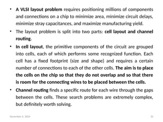
• A VLSI layout problem requires positioning millions of components
and connections on a chip to minimize area, minimize circuit delays,
minimize stray capacitances, and maximize manufacturing yield.
• The layout problem is split into two parts: cell layout and channel
routing.
• In cell layout, the primitive components of the circuit are grouped
into cells, each of which performs some recognized function. Each
cell has a fixed footprint (size and shape) and requires a certain
number of connections to each of the other cells. The aim is to place
the cells on the chip so that they do not overlap and so that there
is room for the connecting wires to be placed between the cells.
• Channel routing finds a specific route for each wire through the gaps
between the cells. These search problems are extremely complex,
but definitely worth solving.
33.
November 6, 202433
• Robot navigation is a generalization of the route-finding problem
described earlier.
• Rather than following distinct paths (such as the roads in Romania), a
robot can roam around, in effect making its own paths.
• For a circular robot moving on a flat surface, the space is essentially two-
dimensional.
• When the robot has arms and legs that must also be controlled, the search
space becomes many-dimensional—one dimension for each joint angle.
• Advanced techniques are required just to make the essentially continuous
search space finite.
• In addition to the complexity of the problem, real robots must also deal
with errors in their sensor readings and motor controls, with partial
observability, and with other agents that might alter the environment.
34.
November 6, 202434
• Automatic assembly sequencing of complex objects (such as
electric motors) by a robot has been standard industry practice
since the 1970s.
• Algorithms first find a feasible assembly sequence and then work to
optimize the process.
• Minimizing the amount of manual human labor on the assembly
line can produce significant savings in time and cost.
• In assembly problems, the aim is to find an order in which to
assemble the parts of some object.
• If the wrong order is chosen, there will be no way to add some part
later in the sequence without undoing some of the work already
done.
• One important assembly problem is Protein design, in which the
goal is to find a sequence of amino acids that will fold into a three-
dimensional protein with the right properties to cure some disease.
November 6, 202436
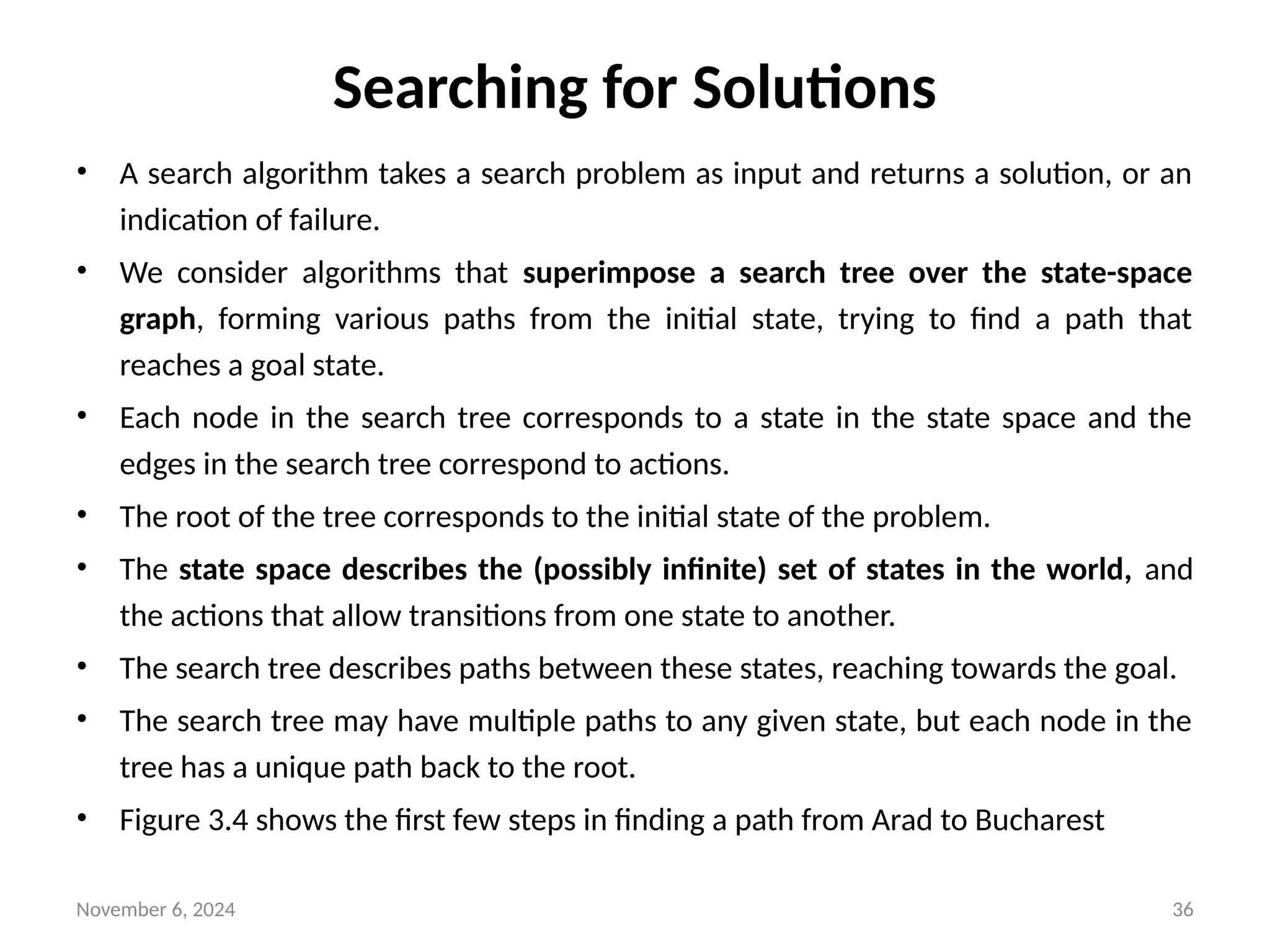
Searching for Solutions
• A search algorithm takes a search problem as input and returns a solution, or an
indication of failure.
• We consider algorithms that superimpose a search tree over the state-space
graph, forming various paths from the initial state, trying to find a path that
reaches a goal state.
• Each node in the search tree corresponds to a state in the state space and the
edges in the search tree correspond to actions.
• The root of the tree corresponds to the initial state of the problem.
• The state space describes the (possibly infinite) set of states in the world, and
the actions that allow transitions from one state to another.
• The search tree describes paths between these states, reaching towards the goal.
• The search tree may have multiple paths to any given state, but each node in the
tree has a unique path back to the root.
• Figure 3.4 shows the first few steps in finding a path from Arad to Bucharest
November 6, 202441
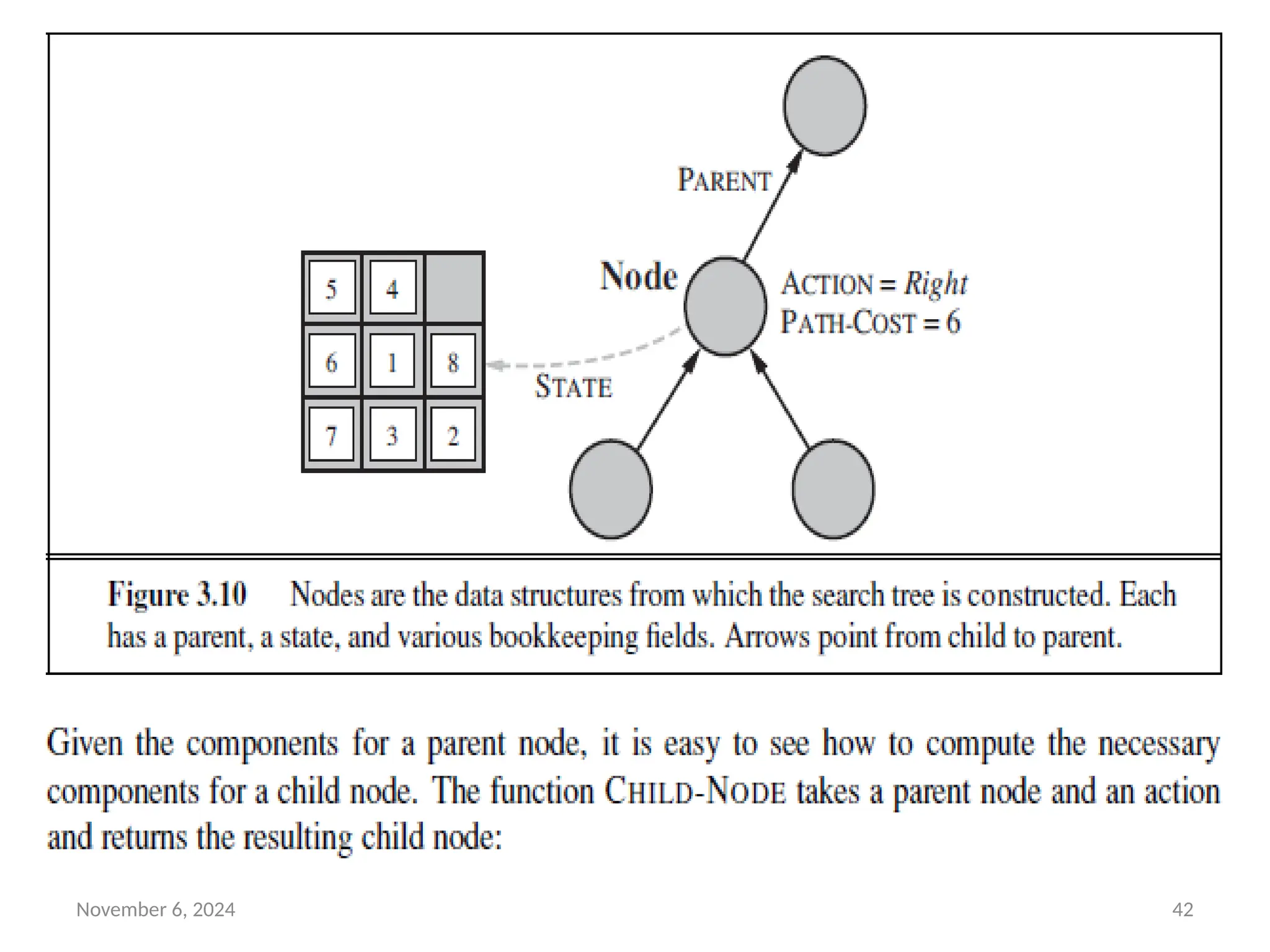
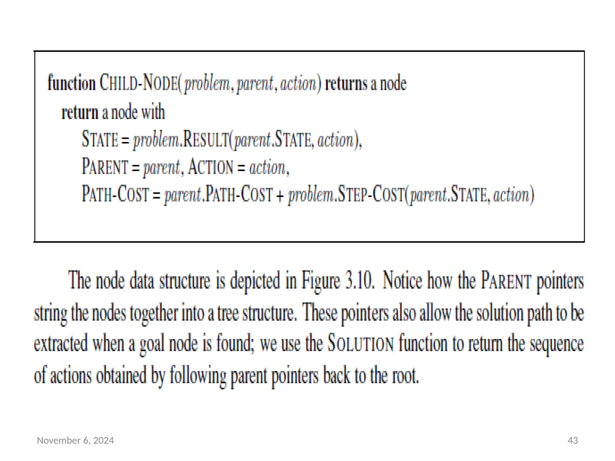
Infrastructure for search algorithms
• Search algorithms require a data structure to keep track of the
search tree that is being constructed.
• For each node n of the tree, we have a structure that contains
four components:
• n.STATE: the state in the state space to which the node
corresponds;
• n.PARENT: the node in the search tree that generated this
node;
• n.ACTION: the action that was applied to the parent to
generate the node;
• n.PATH-COST: the cost, traditionally denoted by g(n), of the
path from the initial state to the node, as indicated by the
parent pointers.
November 6, 202444
• A node is a bookkeeping data structure used to represent the
search tree.
• A state corresponds to a configuration of the world.
• Thus, nodes are on particular paths, as defined by PARENT
pointers, whereas states are not.
• Now that we have nodes, we need somewhere to put them. The
frontier needs to be stored in such a way that the search
algorithm can easily choose the next node to expand according
to its preferred strategy.
• The appropriate data structure for this is a queue.
45.
November 6, 202445
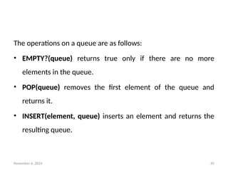
The operations on a queue are as follows:
• EMPTY?(queue) returns true only if there are no more
elements in the queue.
• POP(queue) removes the first element of the queue and
returns it.
• INSERT(element, queue) inserts an element and returns the
resulting queue.
46.
November 6, 202446
• Queues are characterized by the order in which they store the
inserted nodes.
• Three common variants are the first-in, first-out or FIFO
queue, which pops the oldest element of the queue;
• the last-in, first-out or LIFO queue (also known as a stack),
which pops the newest element of the queue;
• and the priority queue, which pops the element of the queue
with the highest priority according to some ordering function
47.
November 6, 202447
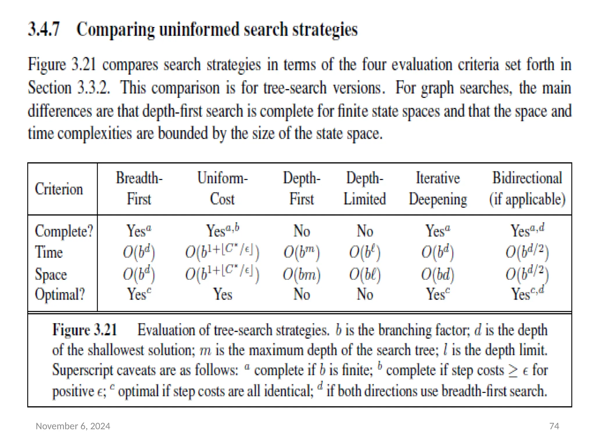
Measuring problem-solving performance
• We can evaluate an algorithm’s performance in four ways:
• Completeness: Is the algorithm guaranteed to find a solution
when there is one?
• Optimality: Does the strategy find the optimal solution?
• Time complexity: How long does it take to find a solution?
• Space complexity: How much memory is needed to perform
the search?
48.
November 6, 202448
• In AI, the graph is represented implicitly by the initial state,
actions, and transition model and is frequently infinite.
• For these reasons, complexity is expressed in terms of three
quantities:
• b, the branching factor or maximum number of successors of
any node;
• d, the depth of the shallowest goal node (i.e., the number of
steps along the path from the root); and
• m, the maximum length of any path in the state space.
• Time is often measured in terms of the number of nodes
generated during the search, and
• space in terms of the maximum number of nodes stored in
memory.
49.
November 6, 202449
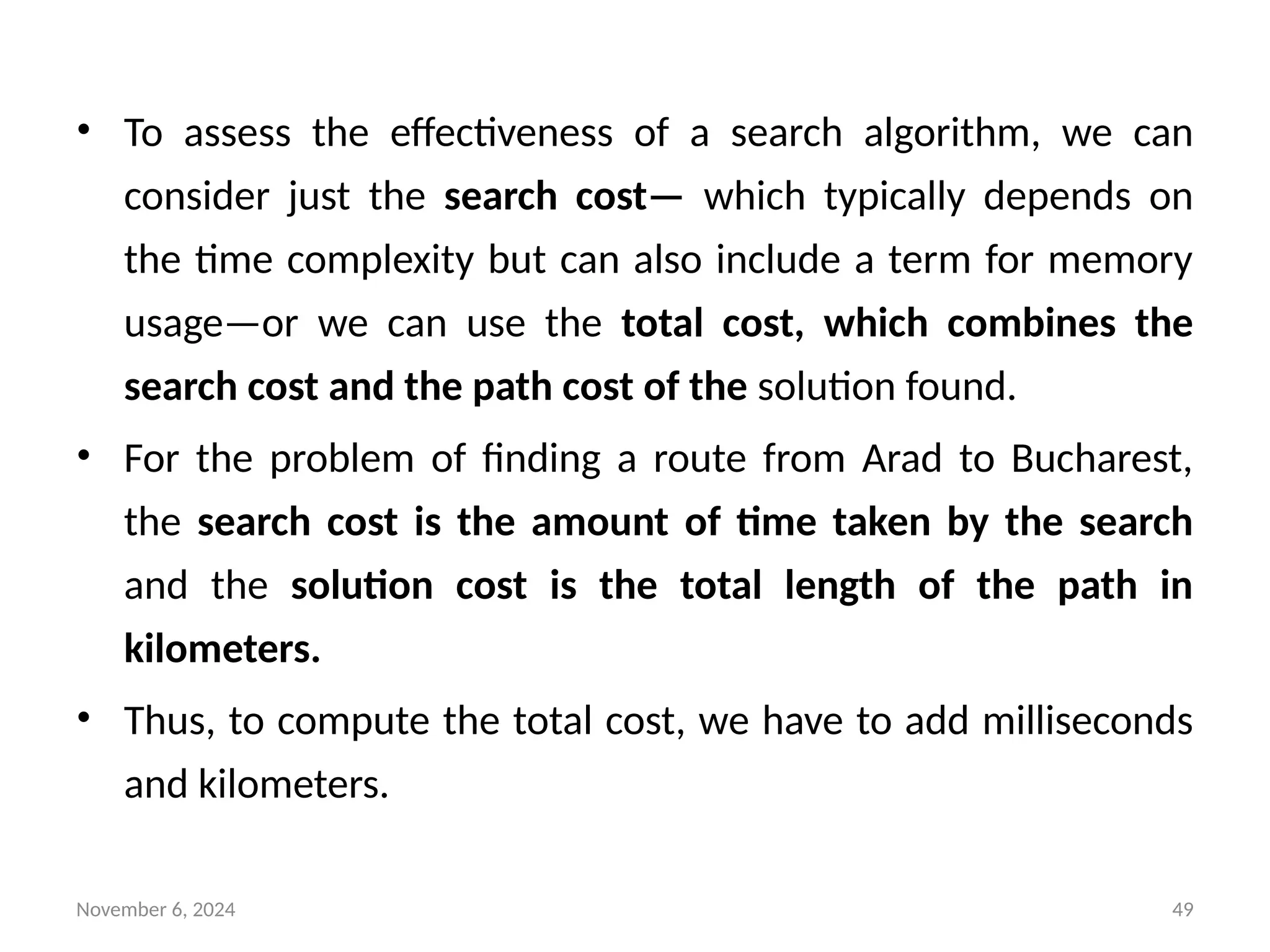
• To assess the effectiveness of a search algorithm, we can
consider just the search cost— which typically depends on
the time complexity but can also include a term for memory
usage—or we can use the total cost, which combines the
search cost and the path cost of the solution found.
• For the problem of finding a route from Arad to Bucharest,
the search cost is the amount of time taken by the search
and the solution cost is the total length of the path in
kilometers.
• Thus, to compute the total cost, we have to add milliseconds
and kilometers.
50.
November 6, 202450
UNINFORMED SEARCH STRATEGIES
• Uninformed search (also called blind search).
• The term means that the strategies have no additional
information about states beyond that provided in the
problem definition.
• All they can do is generate successors and distinguish a goal
state from a non-goal state.
• All search strategies are distinguished by the order in which
nodes are expanded.
• Strategies that know whether one non-goal state is “more
promising” than another are called informed search or
heuristic search strategies;
51.
November 6, 202451
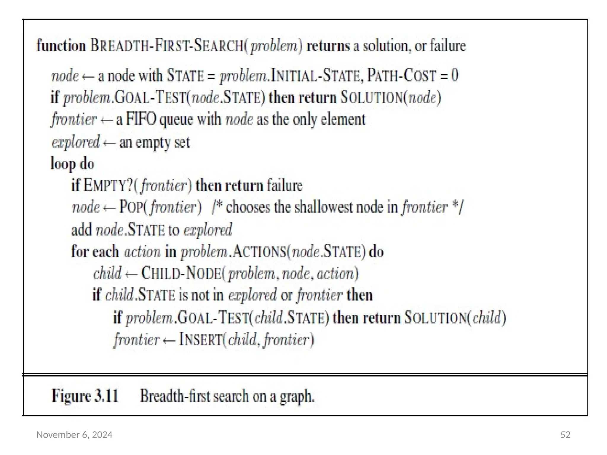
Breadth-first search
• Breadth-first search is a simple strategy in which the root node
is expanded first, then all the successors of the root node are
expanded next, then their successors, and so on.
• Imagine searching a uniform tree where every state has b
successors.
• The root of the search tree generates b nodes at the first level,
each of which generates b more nodes, for a total of b2
at the
second level.
• Each of these generates b more nodes, yielding b3
nodes at the
third level, and so on.
• Now suppose that the solution is at depth d. In the worst case,
it is the last node generated at that level. Then the total
number of nodes generated is
• b + b2
+ b3
+ ・ ・ ・ + bd
= O(bd
) .
November 6, 202453
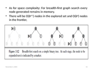
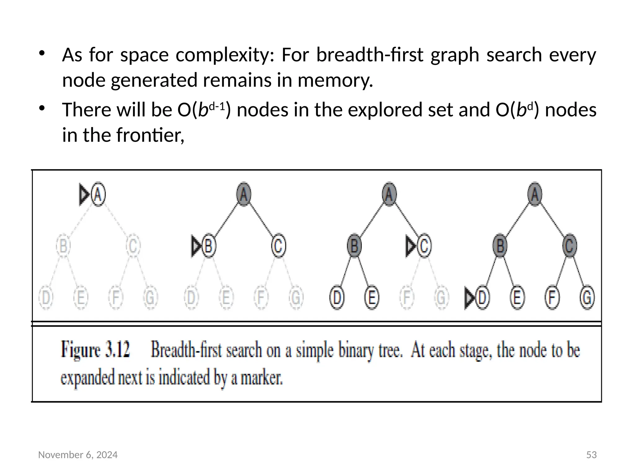
• As for space complexity: For breadth-first graph search every
node generated remains in memory.
• There will be O(bd-1
) nodes in the explored set and O(bd
) nodes
in the frontier,
54.
November 6, 202454
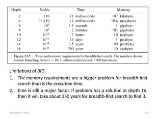
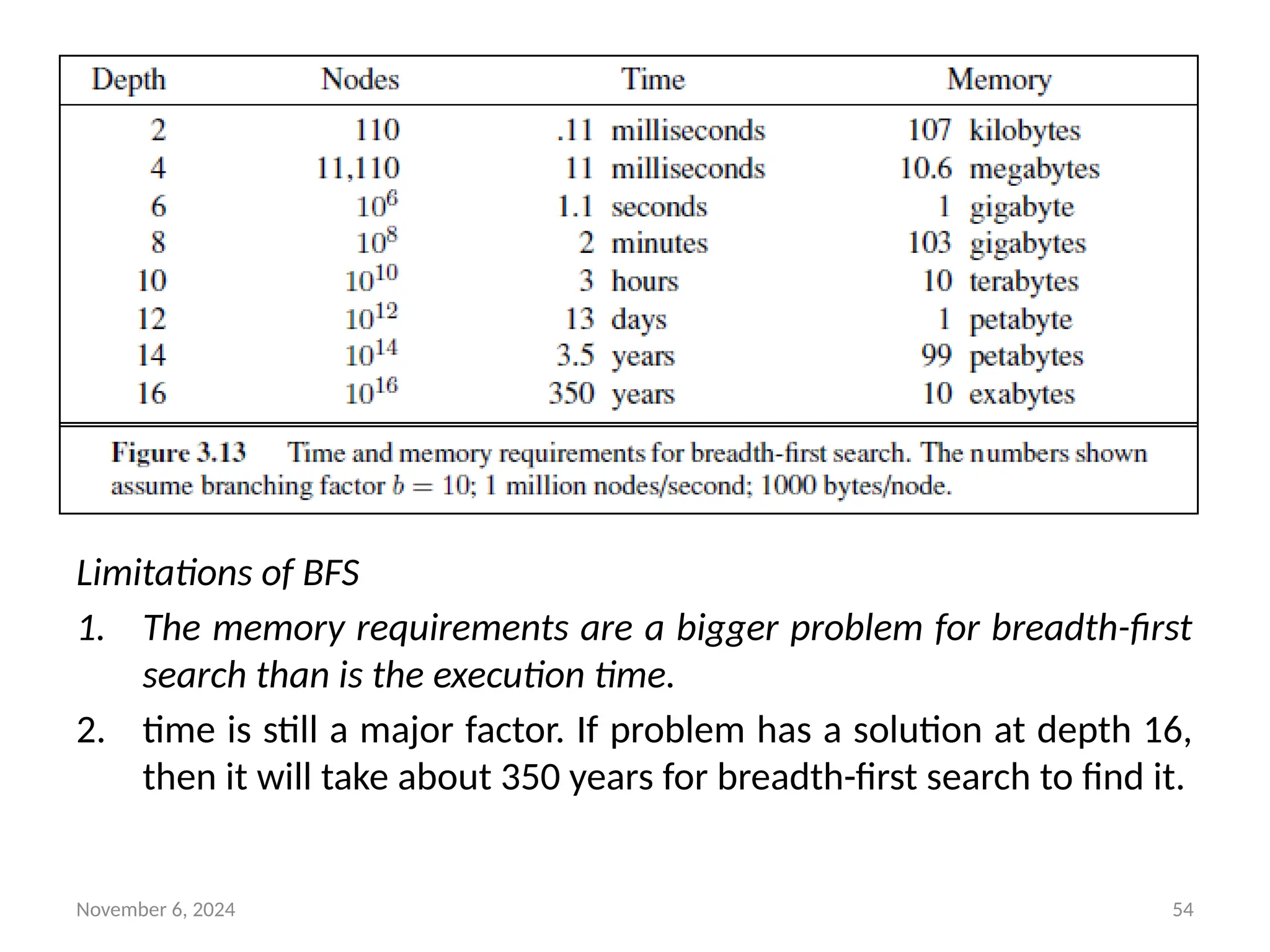
Limitations of BFS
1. The memory requirements are a bigger problem for breadth-first
search than is the execution time.
2. time is still a major factor. If problem has a solution at depth 16,
then it will take about 350 years for breadth-first search to find it.
55.
November 6, 202455
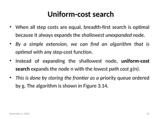
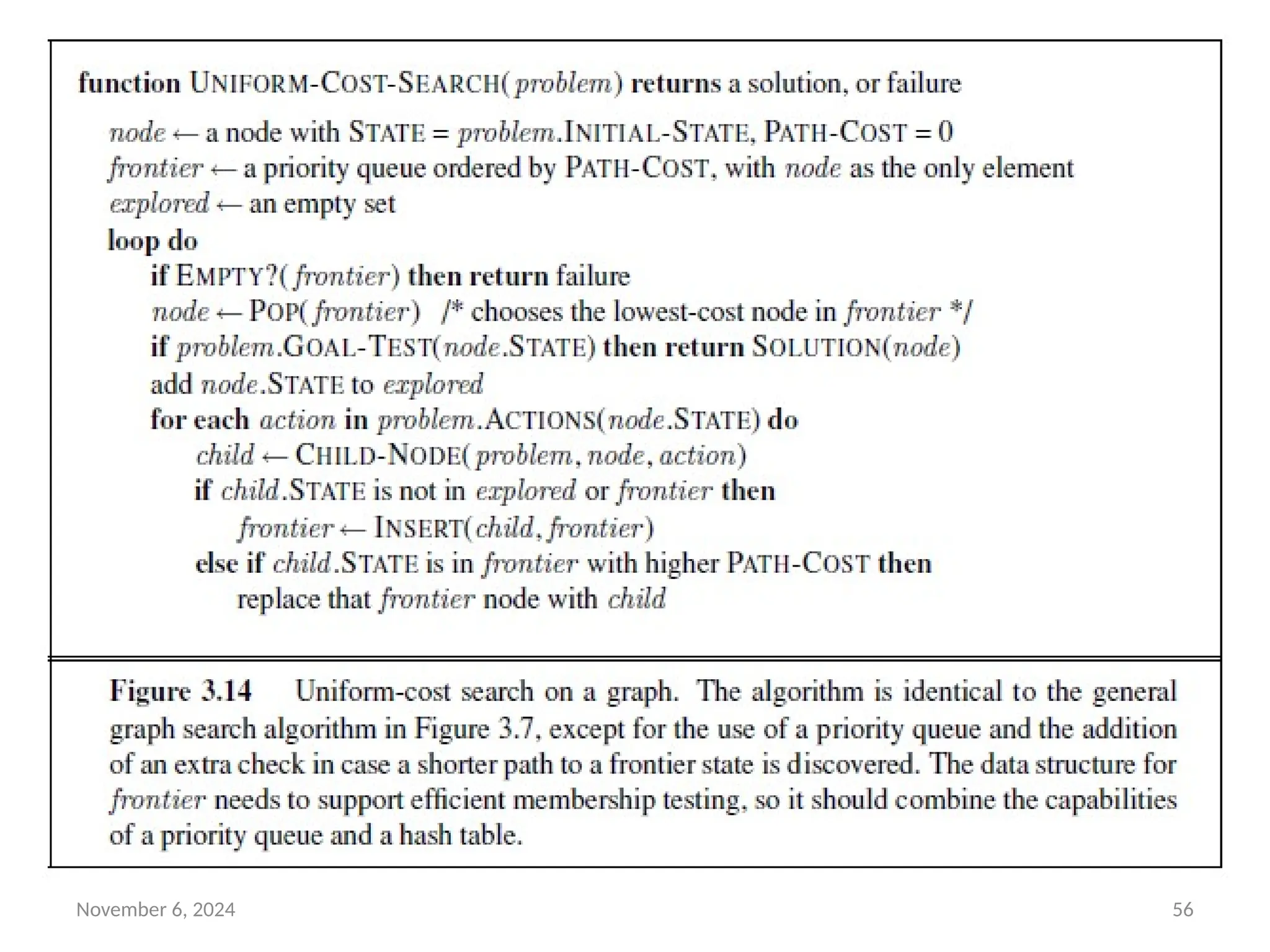
Uniform-cost search
• When all step costs are equal, breadth-first search is optimal
because it always expands the shallowest unexpanded node.
• By a simple extension, we can find an algorithm that is
optimal with any step-cost function.
• Instead of expanding the shallowest node, uniform-cost
search expands the node n with the lowest path cost g(n).
• This is done by storing the frontier as a priority queue ordered
by g. The algorithm is shown in Figure 3.14.
November 6, 202457
• In addition to the ordering of the queue by path cost, there
are two other significant differences from breadth-first search.
1. The goal test is applied to a node when it is selected for
expansion rather than when it is first generated.
2. a test is added in case a better path is found to a node
currently on the frontier.
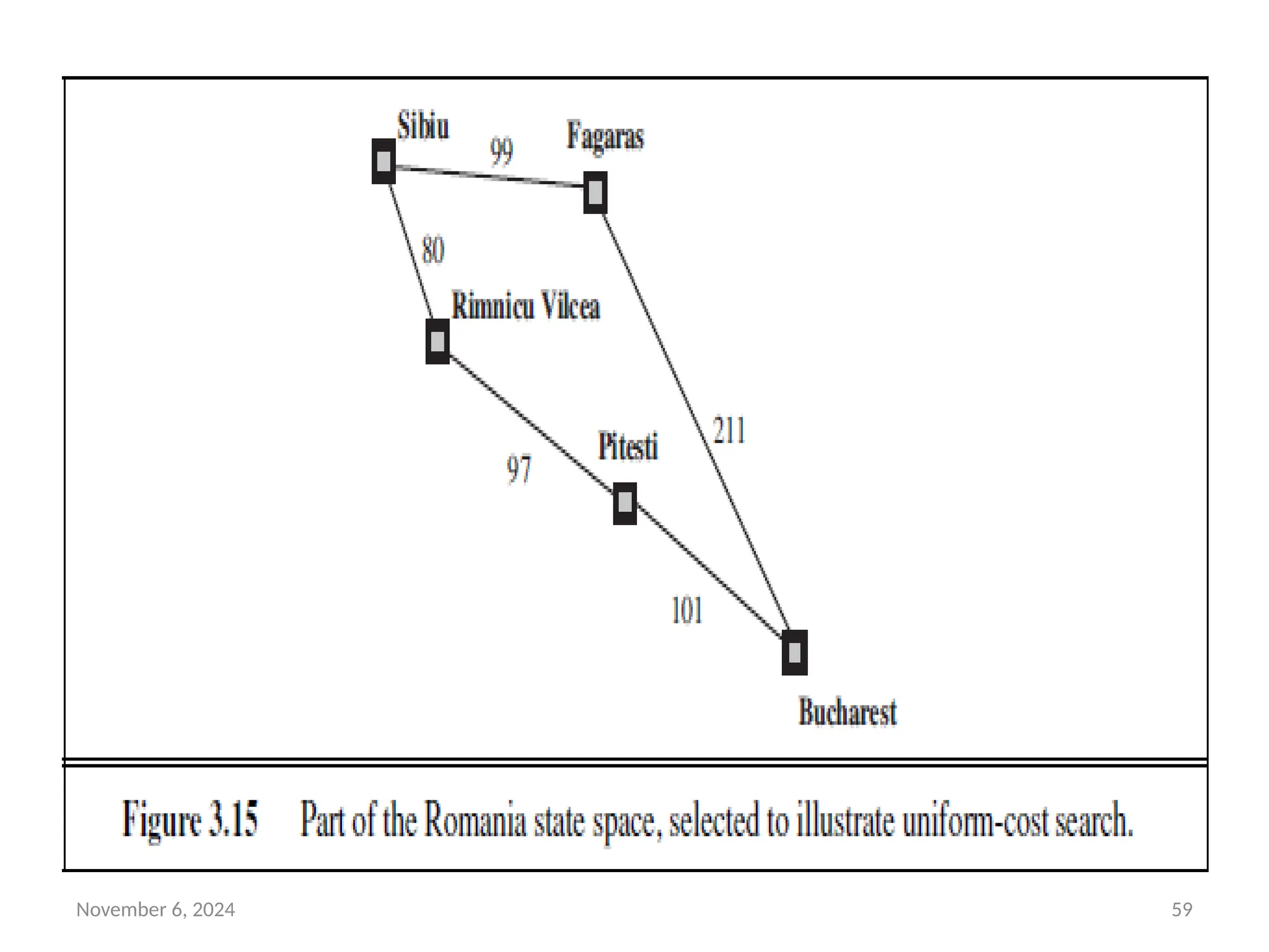
Example:
• The successors of Sibiu are Rimnicu Vilcea and Fagaras, with
costs 80 and 99, respectively.
• The least-cost node, Rimnicu Vilcea, is expanded next, adding
Pitesti with cost 80 + 97=177.
• The least-cost node is now Fagaras, so it is expanded, adding
Bucharest with cost 99+211=310.
58.
November 6, 202458
• Now a goal node has been generated, but uniform-cost search
keeps going, choosing Pitesti for expansion and adding a
second path to Bucharest with cost 80+97+101= 278.
• Now the algorithm checks to see if this new path is better
than the old one; it is, so the old one is discarded. Bucharest,
now with g-cost 278, is selected for expansion and the
solution is returned.
November 6, 202460
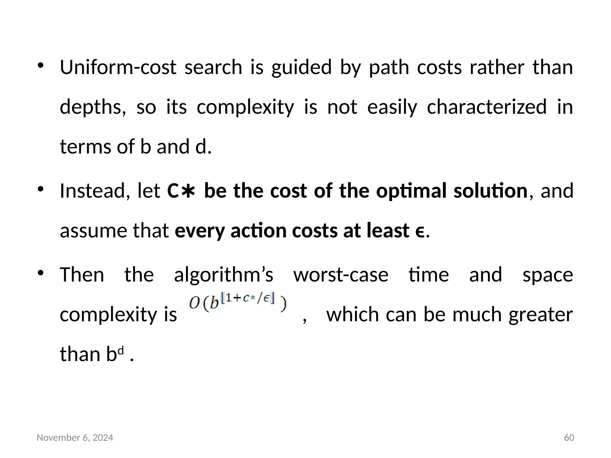
• Uniform-cost search is guided by path costs rather than
depths, so its complexity is not easily characterized in
terms of b and d.
• Instead, let C be the cost of the optimal solution
∗ , and
assume that every action costs at least ϵ.
• Then the algorithm’s worst-case time and space
complexity is , which can be much greater
than bd
.
61.
November 6, 202461
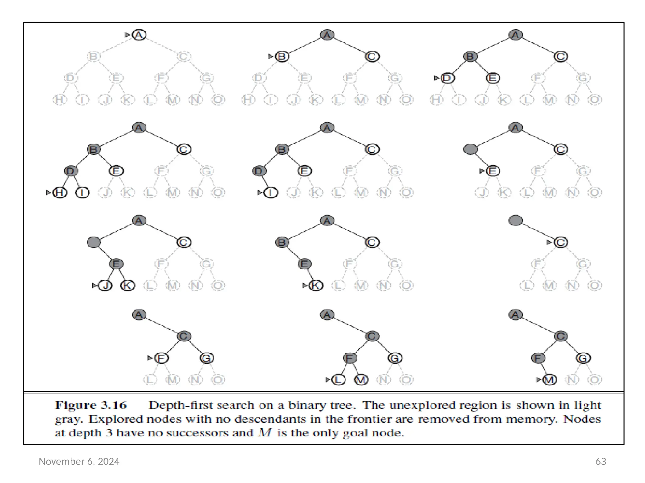
Depth-first search
• Depth-first search always expands the deepest node in the
current frontier of the search tree.
• The progress of the search is illustrated in Figure 3.16.
• The search proceeds immediately to the deepest level of the
search tree, where the nodes have no successors.
• As those nodes are expanded, they are dropped from the
frontier, so then the search “backs up” to the next deepest
node that still has unexplored successors.
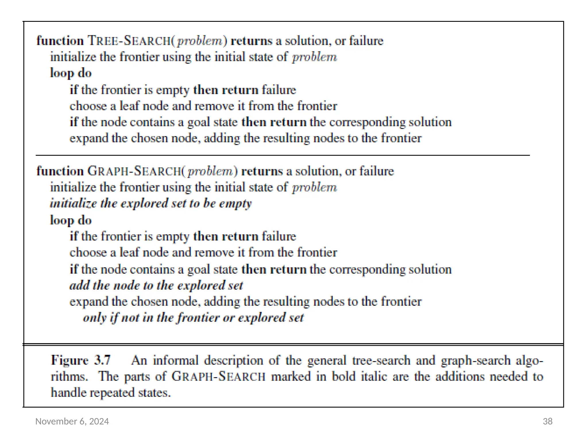
• The depth-first search algorithm is an instance of the graph-
search algorithm in Figure 3.7;
• whereas breadth-first-search uses a FIFO queue, depth-first
search uses a LIFO queue.
November 6, 202464
• The time complexity of depth-first graph search is bounded by
the size of the state space (which may be infinite).
• A depth-first tree search, may generate all of the O(bm
) nodes
in the search tree, where m is the maximum depth of any
node; this can be much greater than the size of the state
space.
• Note that m itself can be much larger than d (the depth of the
shallowest solution) and is infinite if the tree is unbounded.
• For a state space with branching factor b and maximum depth
m, depth-first search requires storage of only O(bm) nodes.
65.
November 6, 202465
• A variant of depth-first search called backtracking search uses
still less memory.
• In backtracking, only one successor is generated at a time
rather than all successors; each partially expanded node
remembers which successor to generate next. In this way,
only O(m) memory is needed
66.
November 6, 202466
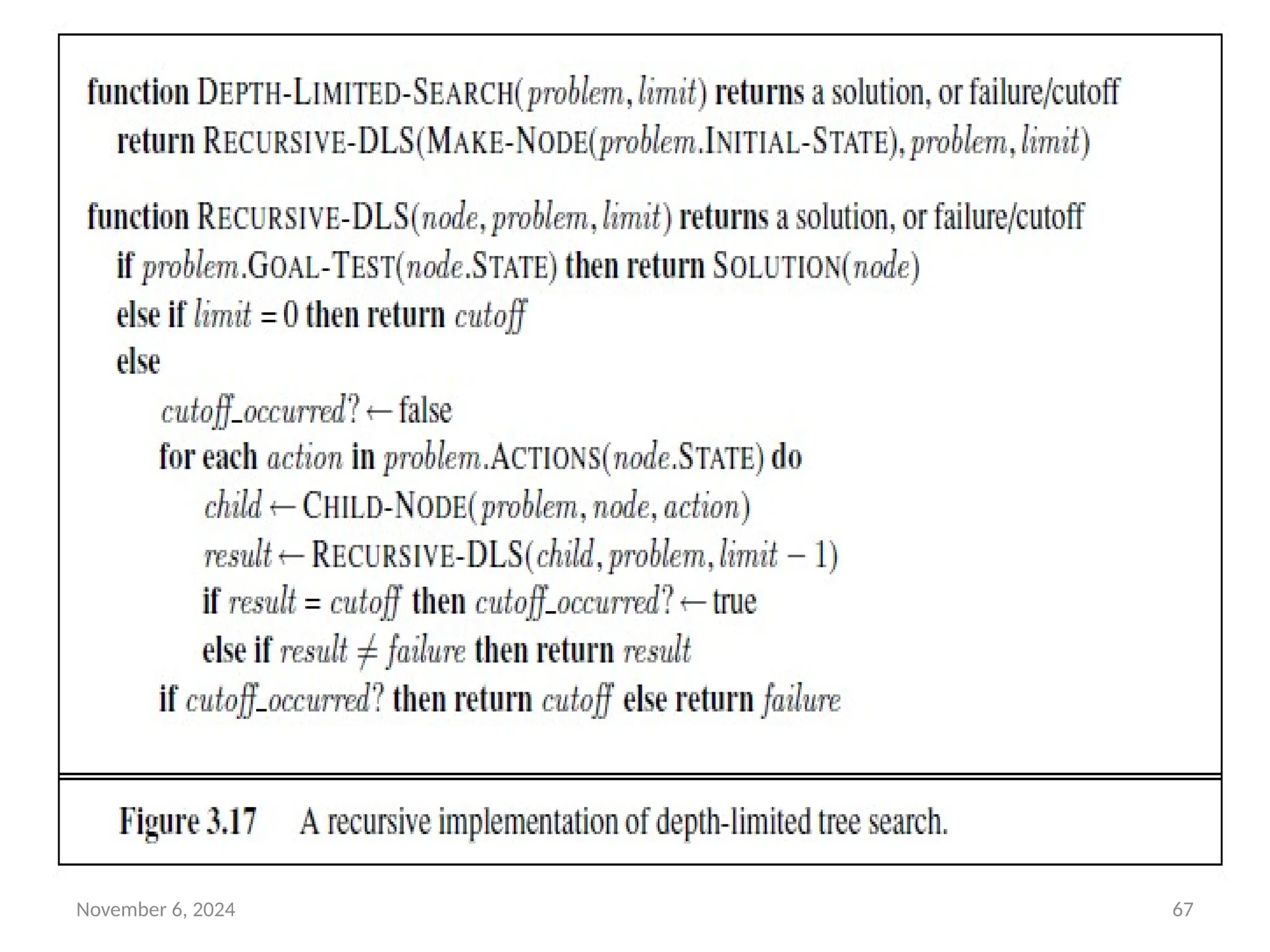
Depth-limited search
• The embarrassing failure of depth-first search in infinite state
spaces can be alleviated by supplying depth-first search with a
predetermined depth limit l.
• That is, nodes at depth l are treated as if they have no
successors. This approach is called depth-limited search.
• The depth limit solves the infinite-path problem.
• Unfortunately, it also introduces an additional source of
incompleteness if we choose l < d, that is, the shallowest goal is
beyond the depth limit.
• Depth-limited search will also be non optimal if we choose l > d.
• Its time complexity is O(bl
) and its space complexity is O(bl
).
• Depth-first search can be viewed as a special case of depth-
limited search with l =∞.
November 6, 202468
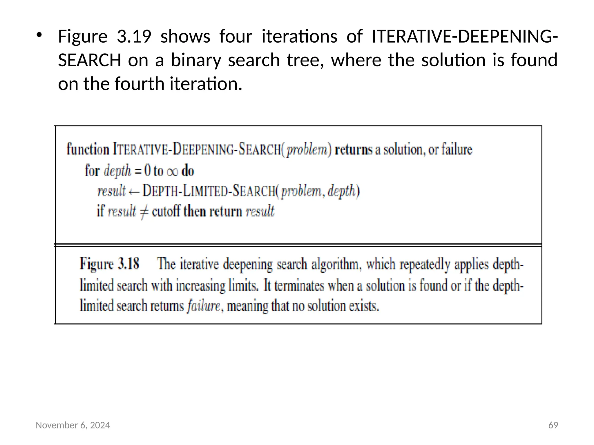
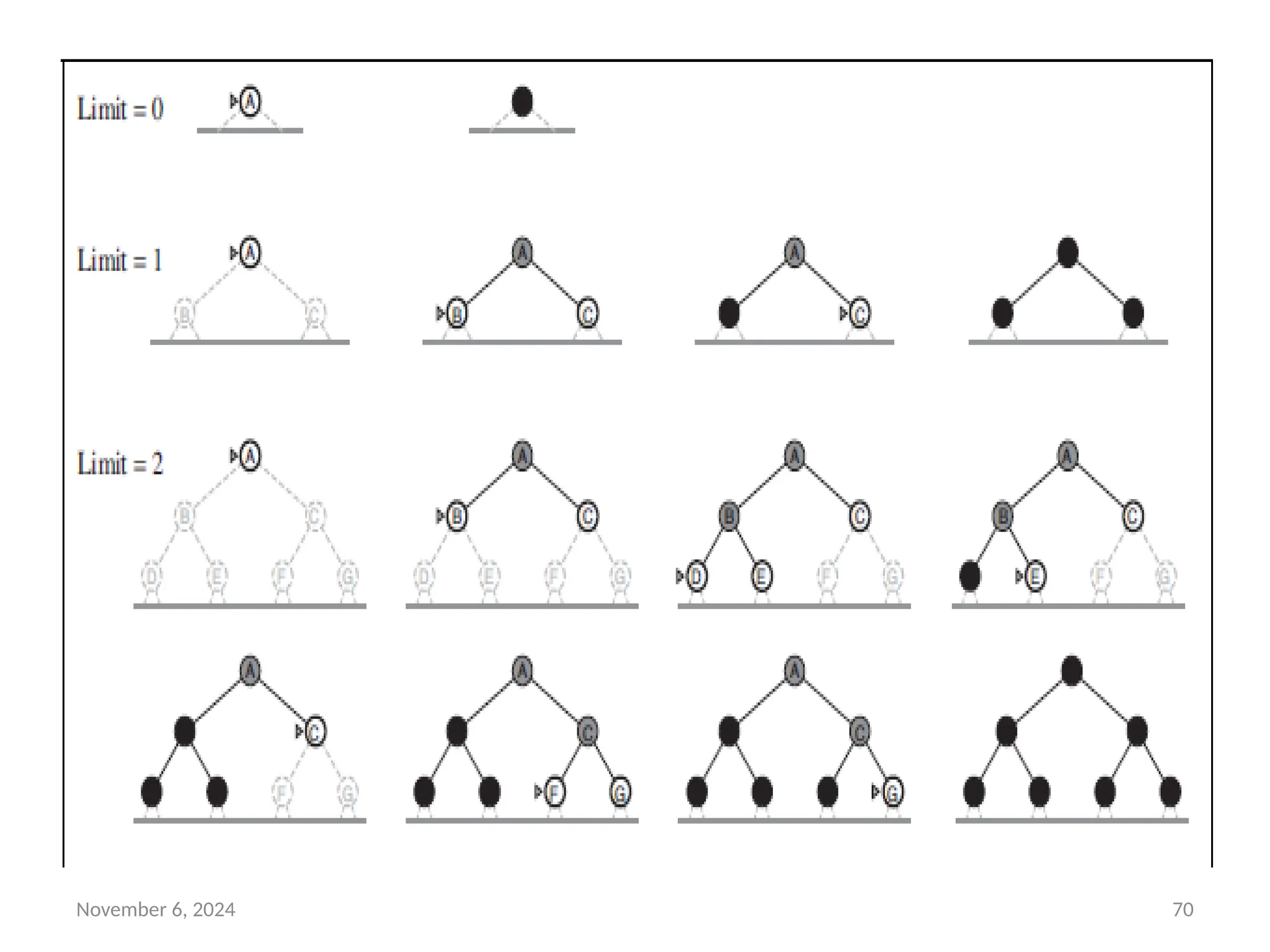
Iterative deepening search
• Iterative deepening search (or iterative deepening depth-first
search) is a general strategy, used in combination with depth-first
tree search, that finds the best depth limit.
• It does this by gradually increasing the limit—first 0, then 1, then
2, and so on—until a goal is found.
• This will occur when the depth limit reaches d, the depth of the
shallowest goal node.
• The algorithm is shown in Figure 3.18.
• Iterative deepening combines the benefits of depth-first and
breadth-first search.
• Like depth-first search, its memory requirements are modest:
O(bd) to be precise.
• Like breadth-first search, it is complete when the branching
factor is finite and optimal when the path cost is a nondecreasing
function of the depth of the node.
69.
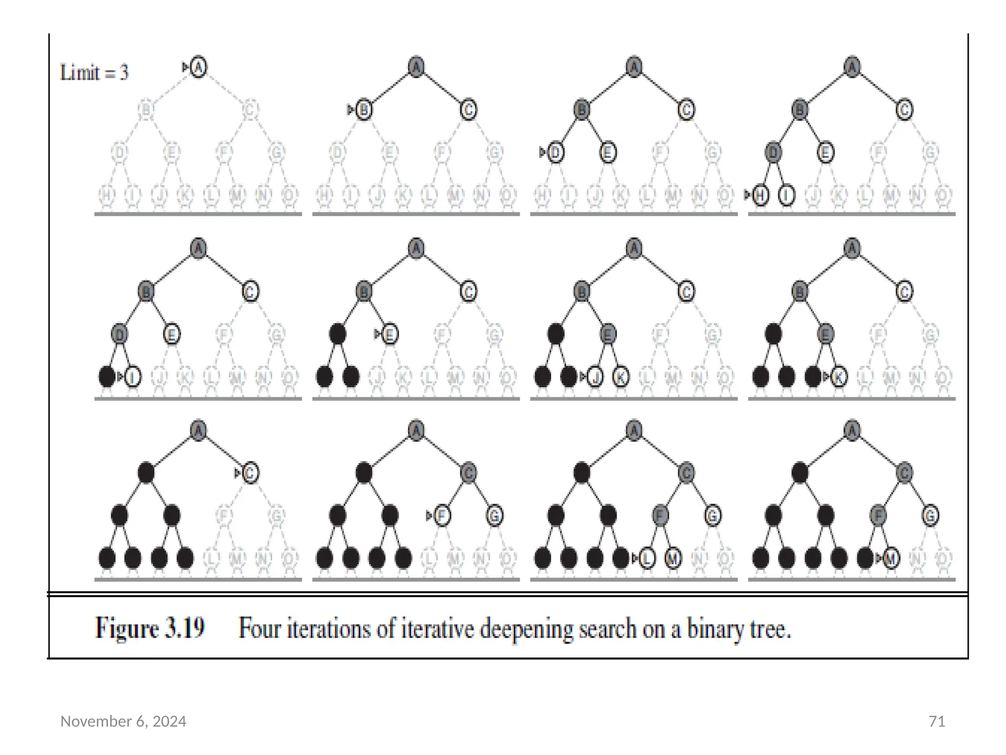
November 6, 202469
• Figure 3.19 shows four iterations of ITERATIVE-DEEPENING-
SEARCH on a binary search tree, where the solution is found
on the fourth iteration.
November 6, 202472
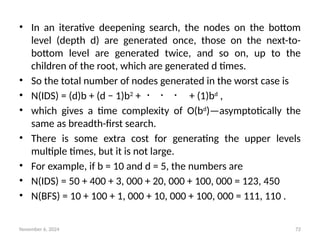
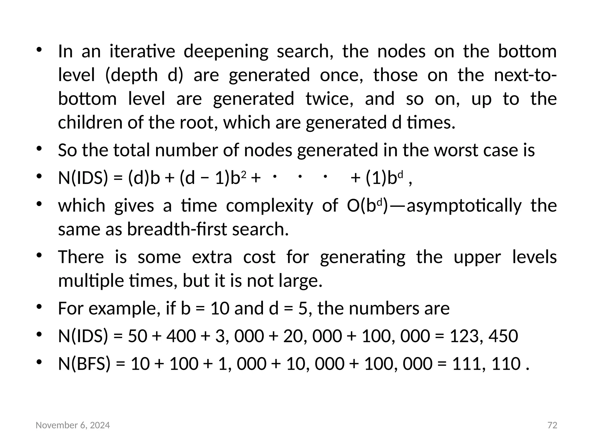
• In an iterative deepening search, the nodes on the bottom
level (depth d) are generated once, those on the next-to-
bottom level are generated twice, and so on, up to the
children of the root, which are generated d times.
• So the total number of nodes generated in the worst case is
• N(IDS) = (d)b + (d − 1)b2
+ ・ ・ ・ + (1)bd
,
• which gives a time complexity of O(bd
)—asymptotically the
same as breadth-first search.
• There is some extra cost for generating the upper levels
multiple times, but it is not large.
• For example, if b = 10 and d = 5, the numbers are
• N(IDS) = 50 + 400 + 3, 000 + 20, 000 + 100, 000 = 123, 450
• N(BFS) = 10 + 100 + 1, 000 + 10, 000 + 100, 000 = 111, 110 .
73.
November 6, 202473
Bidirectional search
• The idea behind bidirectional search is to run two
simultaneous searches—one forward from the initial state and
the other backward from the goal—hoping that the two
searches meet in the middle (Figure 3.20).
• The motivation is that bd/2
+ bd/2
is much less than bd
, or in the
figure, the area of the two small circles is less than the area of
one big circle centered on the start and reaching to the goal.
• Bidirectional search is implemented by replacing the goal test
with a check to see whether the frontiers of the two searches
intersect; if they do, a solution has been found.
• The time complexity of bidirectional search using breadth-first
searches in both directions is O(bd/2
). The space complexity is
also O(bd/2
).