Downloaded 59 times


![Big O Notation
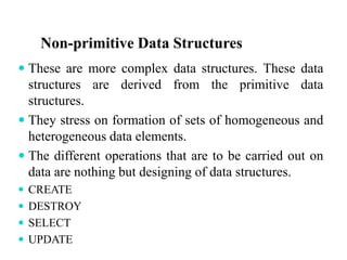
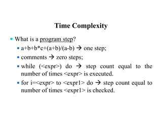
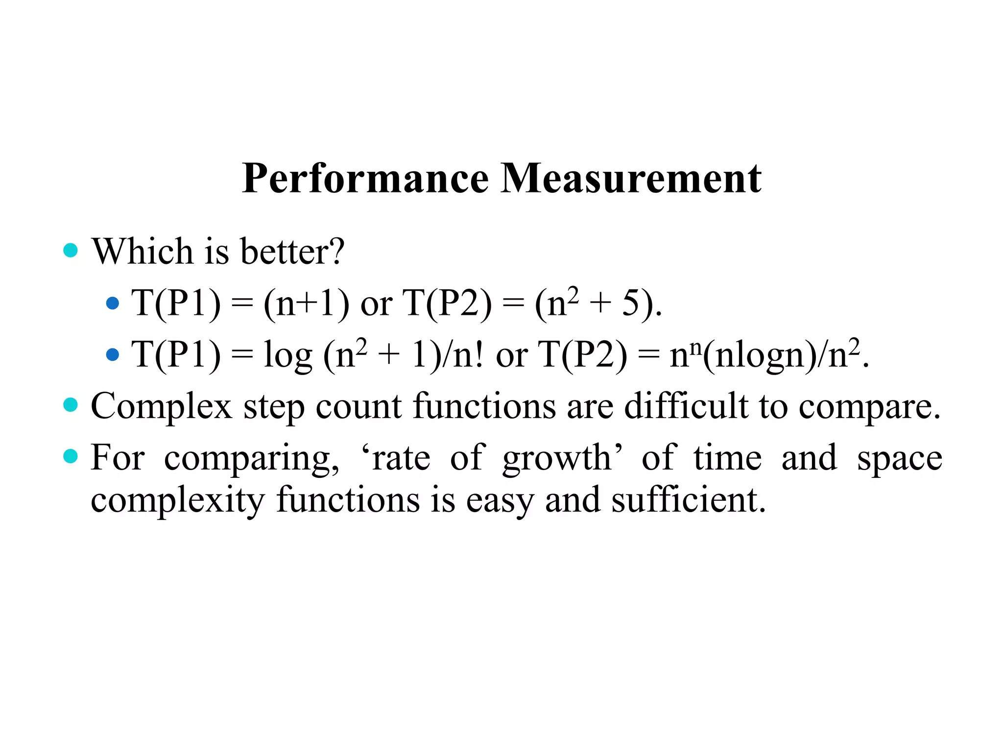
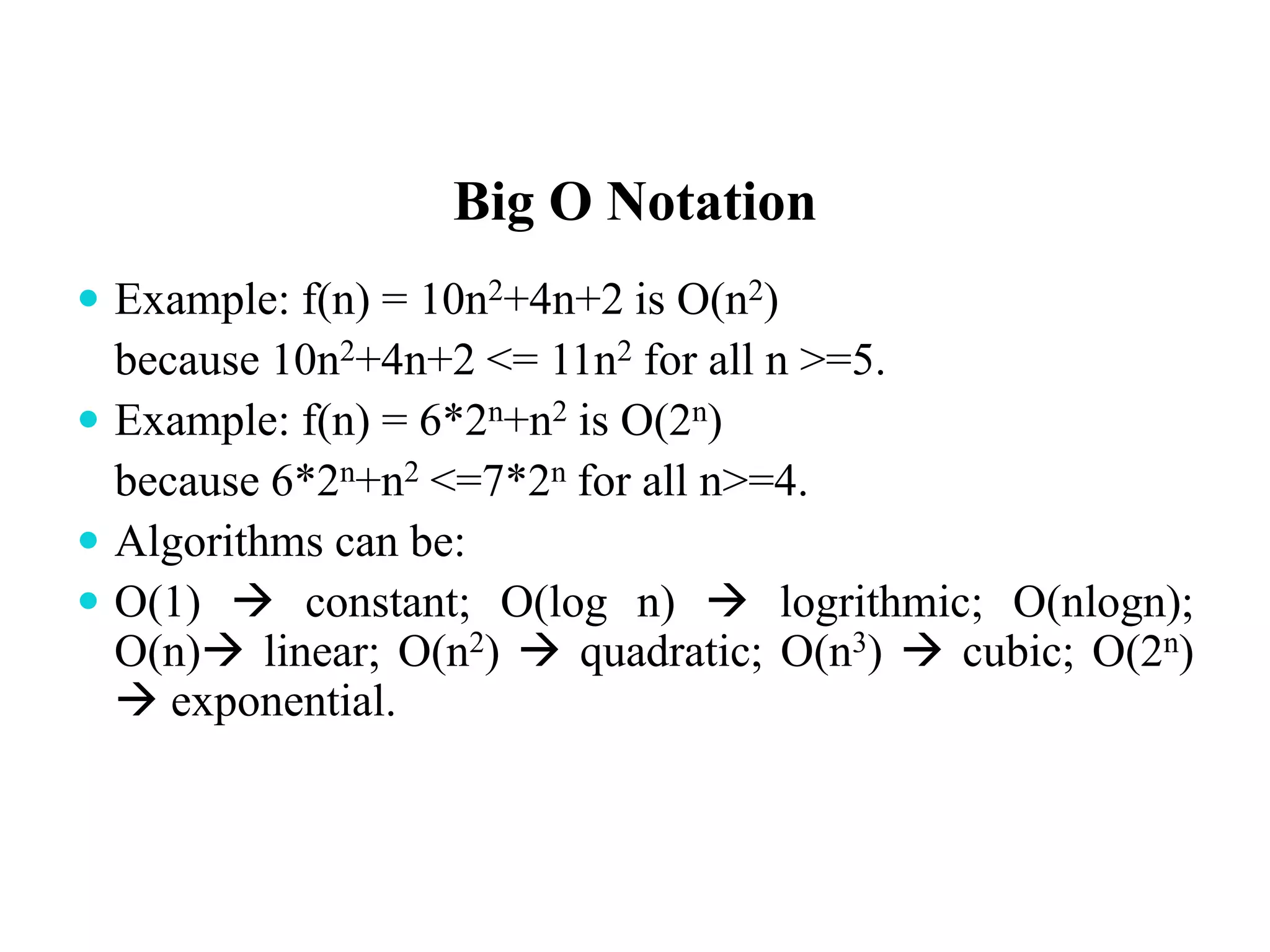
Big O of a function gives us ‘rate of growth’ of the
step count function f(n), in terms of a simple function
g(n), which is easy to compare.
Definition:
[Big O] The function f(n) = O(g(n)) (big ‘oh’ of g of
n) if
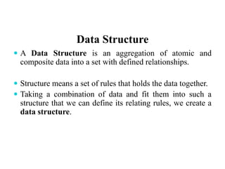
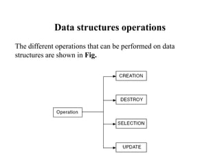
there exist positive constants c and n0 such that f(n) <=
c*g(n) for all n, n>=n0. See graph on next slide.
Example: f(n) = 3n+2 is O(n) because 3n+2 <= 4n for
all n >= 2. c = 4, n0 = 2. Here g(n) = n.](https://image.slidesharecdn.com/bsccs-iidfsu-1introductiontodatastructure-150317031635-conversion-gate01/85/Bsc-cs-ii-dfs-u-1-introduction-to-data-structure-16-320.jpg)
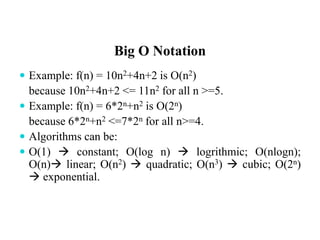
![Big O Notation[1]
= n0](https://image.slidesharecdn.com/bsccs-iidfsu-1introductiontodatastructure-150317031635-conversion-gate01/85/Bsc-cs-ii-dfs-u-1-introduction-to-data-structure-17-320.jpg)


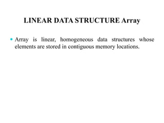
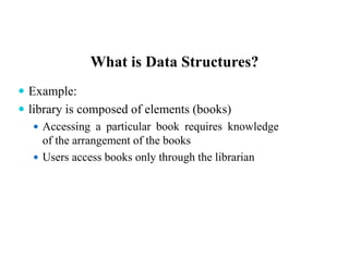
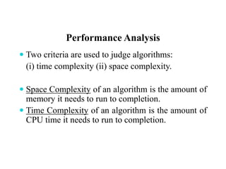
![Initializing Arrays
Using a loop:
for (int i = 0; i < myList.length; i++)
myList[i] = i;
Declaring, creating, initializing in one step:
double[] myList = {1.9, 2.9, 3.4, 3.5};
This shorthand syntax must be in one statement.](https://image.slidesharecdn.com/bsccs-iidfsu-1introductiontodatastructure-150317031635-conversion-gate01/85/Bsc-cs-ii-dfs-u-1-introduction-to-data-structure-23-320.jpg)
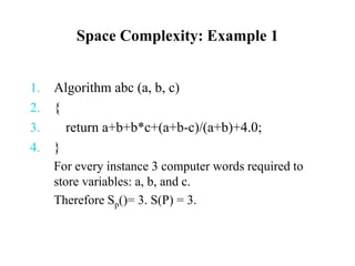
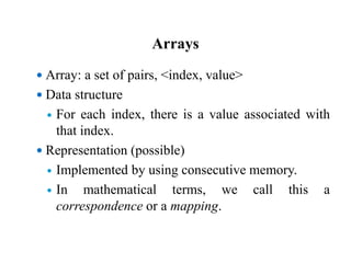
![Declaring and Creating in One Step
datatype[] arrayname = new
datatype[arraySize];
double[] myList = new double[10];
datatype arrayname[] = new
datatype[arraySize];
double myList[] = new double[10];](https://image.slidesharecdn.com/bsccs-iidfsu-1introductiontodatastructure-150317031635-conversion-gate01/85/Bsc-cs-ii-dfs-u-1-introduction-to-data-structure-24-320.jpg)
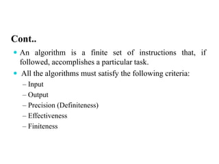
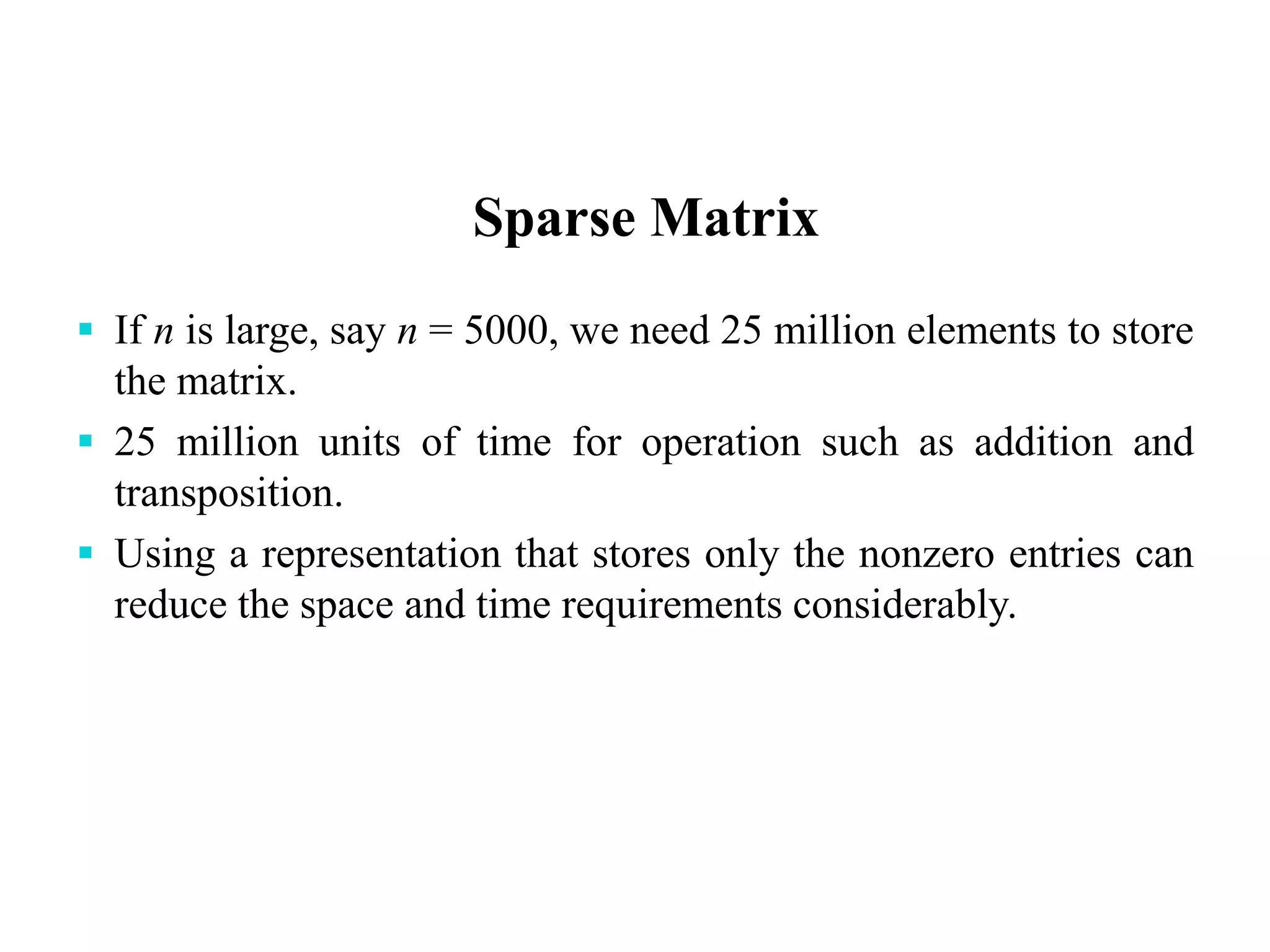
![Sparse Matrix[2]
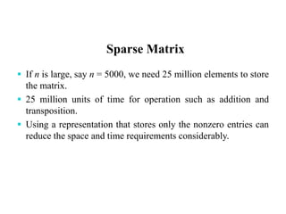
A sparse matrix is a matrix that has many zero entries.
0002800
0000091
000000
006000
0003110
150220015
• This is a __×__ matrix.
• There are _____ entries.
• There are _____ nonzero entries.
• There are _____ zero entries.
Consider we use a 2D array to represent a n×n sparse matrix. How many entries
are required? _____ entries. The space complexity is O( ).](https://image.slidesharecdn.com/bsccs-iidfsu-1introductiontodatastructure-150317031635-conversion-gate01/85/Bsc-cs-ii-dfs-u-1-introduction-to-data-structure-25-320.jpg)
![Exercise : Bubble Sort
int[] myList = {2, 9, 5, 4, 8, 1, 6}; // Unsorted
Pass 1: 2, 5, 4, 8, 1, 6, 9
Pass 2: 2, 4, 5, 1, 6, 8, 9
Pass 3: 2, 4, 1, 5, 6, 8, 9
Pass 4: 2, 1, 4, 5, 6, 8, 9
Pass 5: 1, 2, 4, 5, 6, 8, 9
Pass 6: 1, 2, 4, 5, 6, 8, 9](https://image.slidesharecdn.com/bsccs-iidfsu-1introductiontodatastructure-150317031635-conversion-gate01/85/Bsc-cs-ii-dfs-u-1-introduction-to-data-structure-30-320.jpg)
![Tower of Hanoi[3]
The Objective is to transfer the entire tower to one of
the other pegs.
However you can only move one disk at a time and
you can never stack a larger disk onto a smaller disk.
Try to solve it in fewest possible moves.](https://image.slidesharecdn.com/bsccs-iidfsu-1introductiontodatastructure-150317031635-conversion-gate01/85/Bsc-cs-ii-dfs-u-1-introduction-to-data-structure-31-320.jpg)
![Tower of Hanoi[4]](https://image.slidesharecdn.com/bsccs-iidfsu-1introductiontodatastructure-150317031635-conversion-gate01/85/Bsc-cs-ii-dfs-u-1-introduction-to-data-structure-32-320.jpg)


![Big O Notation
Big O of a function gives us ‘rate of growth’ of the
step count function f(n), in terms of a simple function
g(n), which is easy to compare.
Definition:
[Big O] The function f(n) = O(g(n)) (big ‘oh’ of g of
n) if
there exist positive constants c and n0 such that f(n) <=
c*g(n) for all n, n>=n0. See graph on next slide.
Example: f(n) = 3n+2 is O(n) because 3n+2 <= 4n for
all n >= 2. c = 4, n0 = 2. Here g(n) = n.](https://image.slidesharecdn.com/bsccs-iidfsu-1introductiontodatastructure-150317031635-conversion-gate01/75/Bsc-cs-ii-dfs-u-1-introduction-to-data-structure-16-2048.jpg)
![Big O Notation[1]
= n0](https://image.slidesharecdn.com/bsccs-iidfsu-1introductiontodatastructure-150317031635-conversion-gate01/75/Bsc-cs-ii-dfs-u-1-introduction-to-data-structure-17-2048.jpg)

![Initializing Arrays
Using a loop:
for (int i = 0; i < myList.length; i++)
myList[i] = i;
Declaring, creating, initializing in one step:
double[] myList = {1.9, 2.9, 3.4, 3.5};
This shorthand syntax must be in one statement.](https://image.slidesharecdn.com/bsccs-iidfsu-1introductiontodatastructure-150317031635-conversion-gate01/75/Bsc-cs-ii-dfs-u-1-introduction-to-data-structure-23-2048.jpg)
![Declaring and Creating in One Step
datatype[] arrayname = new
datatype[arraySize];
double[] myList = new double[10];
datatype arrayname[] = new
datatype[arraySize];
double myList[] = new double[10];](https://image.slidesharecdn.com/bsccs-iidfsu-1introductiontodatastructure-150317031635-conversion-gate01/75/Bsc-cs-ii-dfs-u-1-introduction-to-data-structure-24-2048.jpg)
![Sparse Matrix[2]
A sparse matrix is a matrix that has many zero entries.
0002800
0000091
000000
006000
0003110
150220015
• This is a __×__ matrix.
• There are _____ entries.
• There are _____ nonzero entries.
• There are _____ zero entries.
Consider we use a 2D array to represent a n×n sparse matrix. How many entries
are required? _____ entries. The space complexity is O( ).](https://image.slidesharecdn.com/bsccs-iidfsu-1introductiontodatastructure-150317031635-conversion-gate01/75/Bsc-cs-ii-dfs-u-1-introduction-to-data-structure-25-2048.jpg)


![Exercise : Bubble Sort
int[] myList = {2, 9, 5, 4, 8, 1, 6}; // Unsorted
Pass 1: 2, 5, 4, 8, 1, 6, 9
Pass 2: 2, 4, 5, 1, 6, 8, 9
Pass 3: 2, 4, 1, 5, 6, 8, 9
Pass 4: 2, 1, 4, 5, 6, 8, 9
Pass 5: 1, 2, 4, 5, 6, 8, 9
Pass 6: 1, 2, 4, 5, 6, 8, 9](https://image.slidesharecdn.com/bsccs-iidfsu-1introductiontodatastructure-150317031635-conversion-gate01/75/Bsc-cs-ii-dfs-u-1-introduction-to-data-structure-30-2048.jpg)
![Tower of Hanoi[3]
The Objective is to transfer the entire tower to one of
the other pegs.
However you can only move one disk at a time and
you can never stack a larger disk onto a smaller disk.
Try to solve it in fewest possible moves.](https://image.slidesharecdn.com/bsccs-iidfsu-1introductiontodatastructure-150317031635-conversion-gate01/75/Bsc-cs-ii-dfs-u-1-introduction-to-data-structure-31-2048.jpg)
![Tower of Hanoi[4]](https://image.slidesharecdn.com/bsccs-iidfsu-1introductiontodatastructure-150317031635-conversion-gate01/75/Bsc-cs-ii-dfs-u-1-introduction-to-data-structure-32-2048.jpg)

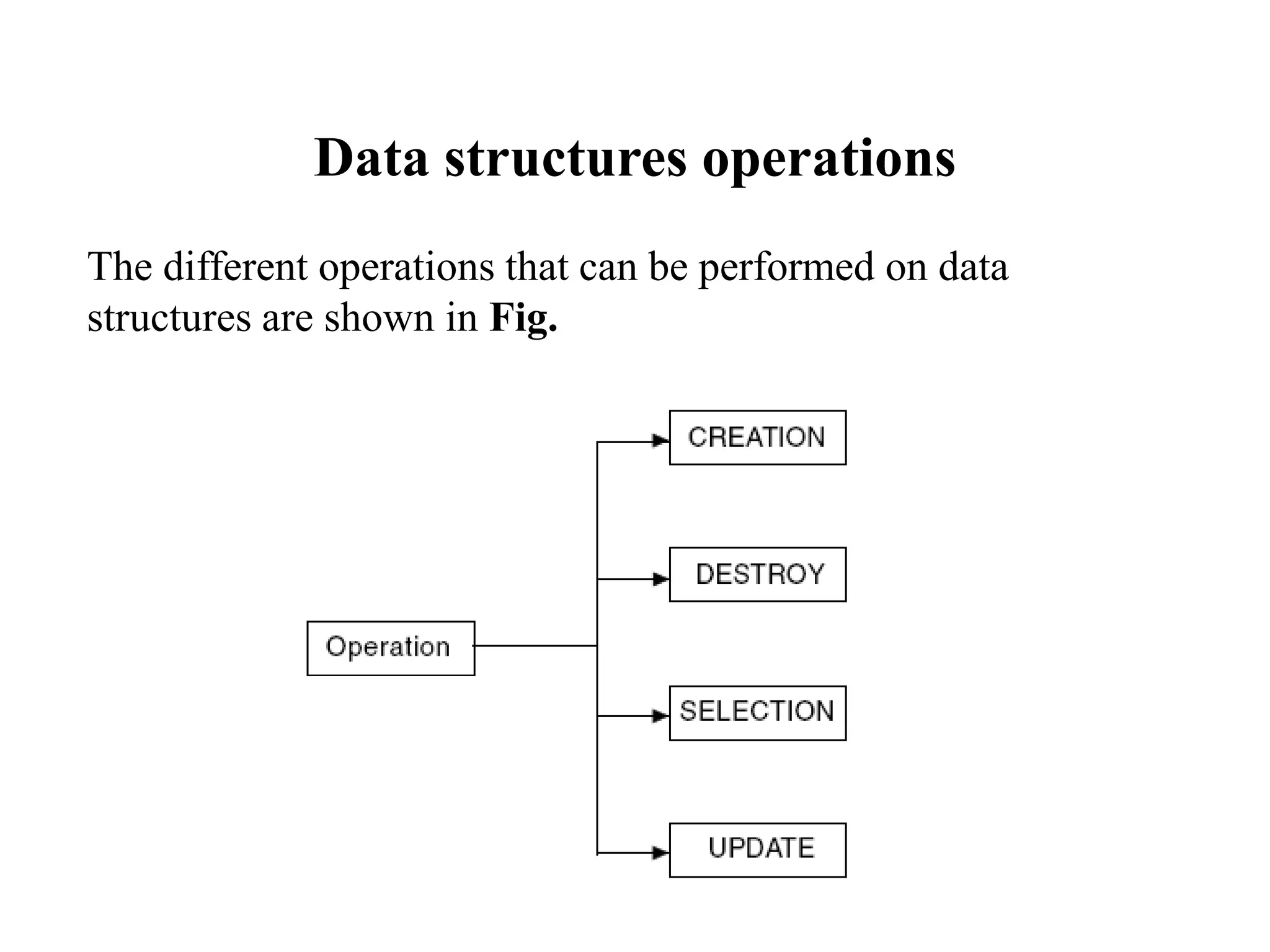
This document provides an introduction to data structures. It defines data structures as a way of organizing and storing data in a computer so it can be used efficiently. The document discusses different types of data structures including primitive, non-primitive, linear and non-linear structures. It provides examples of common data structures like arrays, linked lists, stacks, queues and trees. It also covers important concepts like time and space complexity analysis and Big O notation for analyzing algorithm efficiency.


