Downloaded 943 times

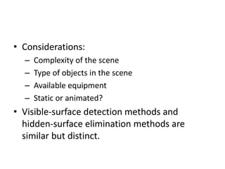


The document provides an overview of visible-surface detection methods, classifying algorithms into object-space and image-space methods, each with distinct approaches and complexities. It discusses the depth-buffer algorithm, its implementation, pros, and cons, and highlights key concepts such as correct visibility, coherence, and the requirements for displaying 3D surfaces on a 2D plane. Additionally, it poses several questions to assess understanding of the discussed methods and their differences.
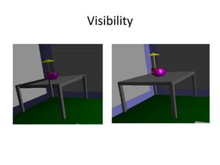
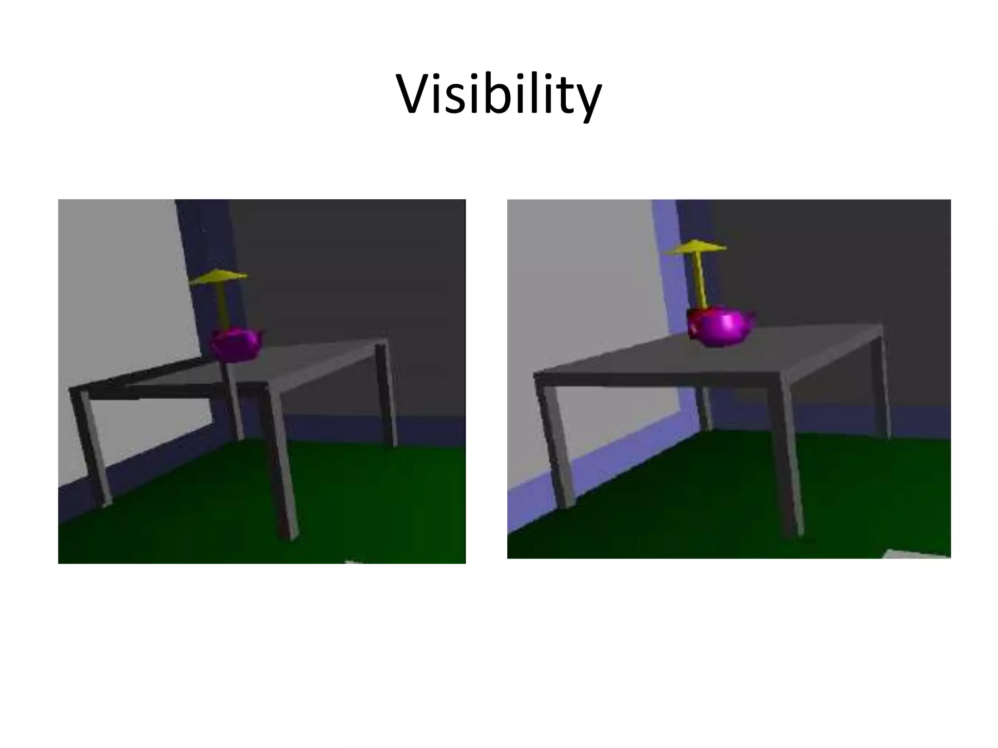
Introduction to visible-surface detection methods, importance of correct visibility, and characteristics of various algorithms.
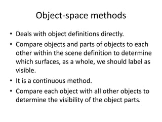
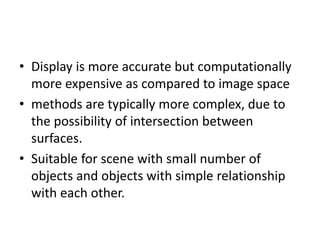
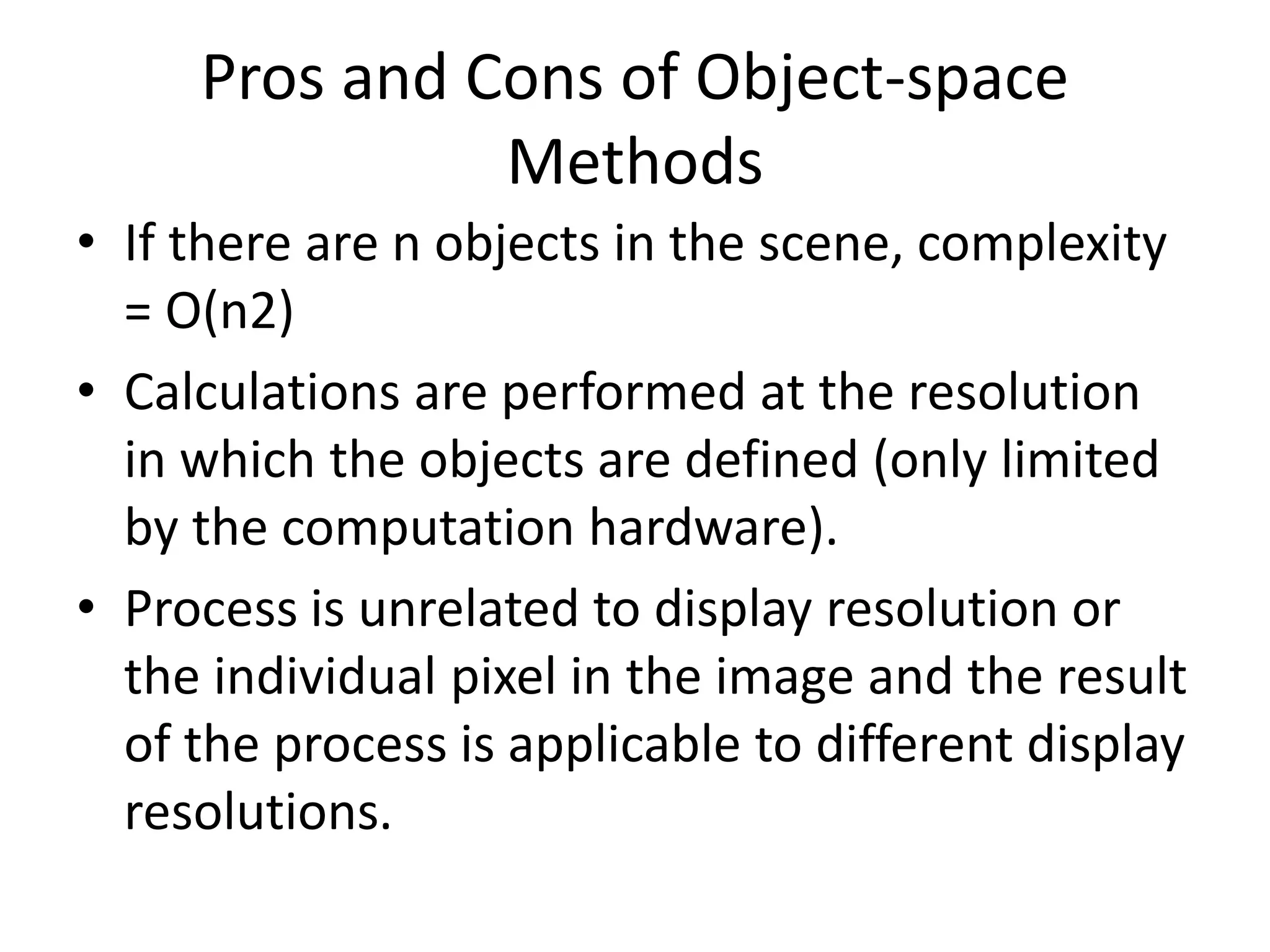
Classification of algorithms into object-space and image-space methods, discussing their pros and cons.
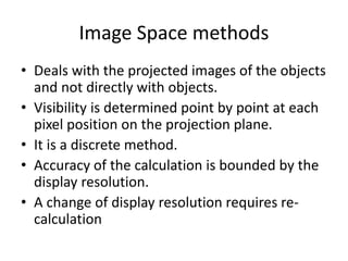
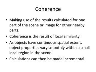
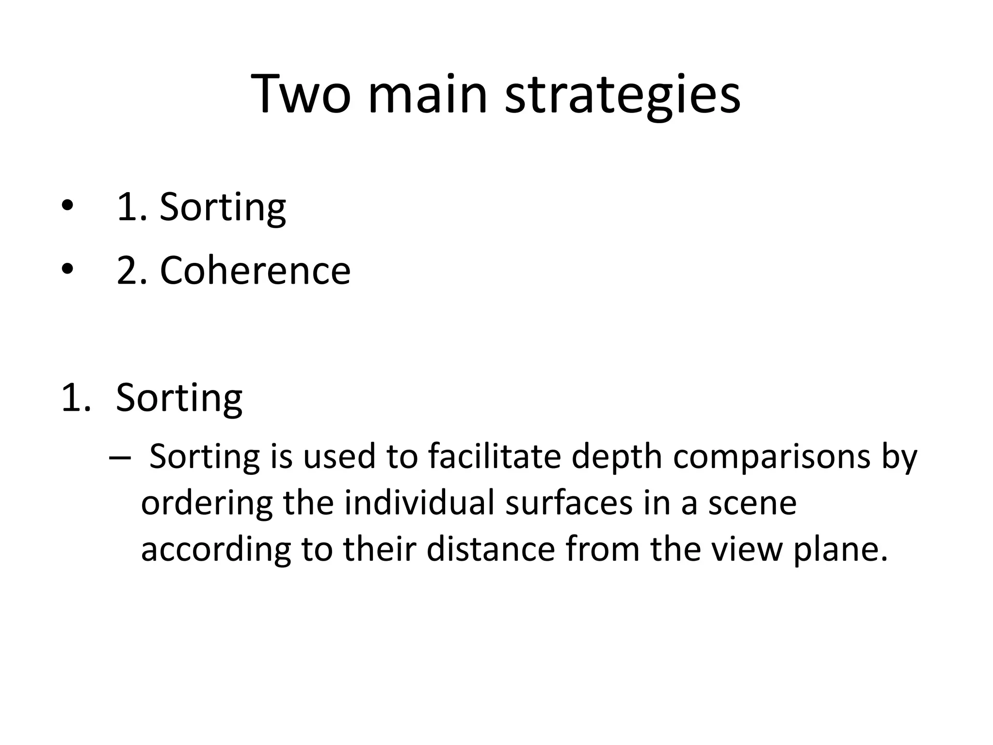
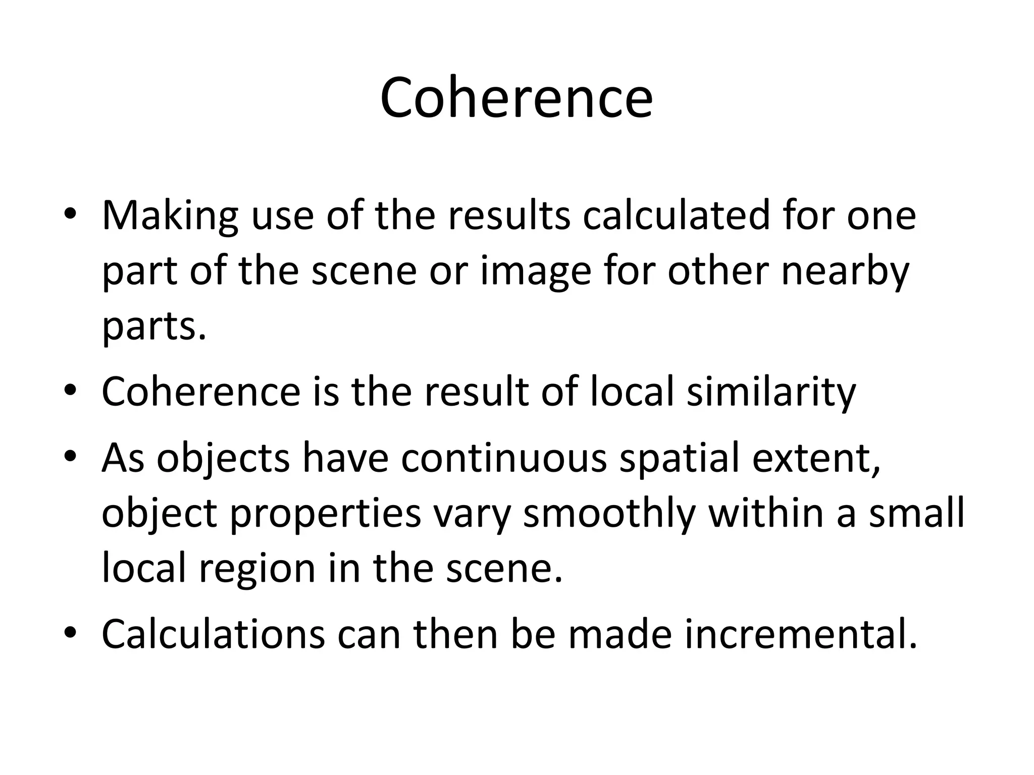
Focuses on image-space methods, their point-by-point visibility determination and strategies of sorting and coherence.
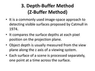
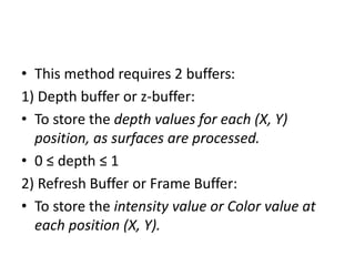
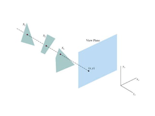
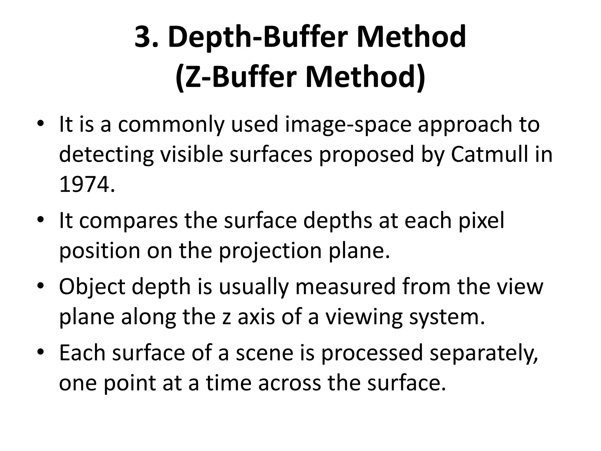
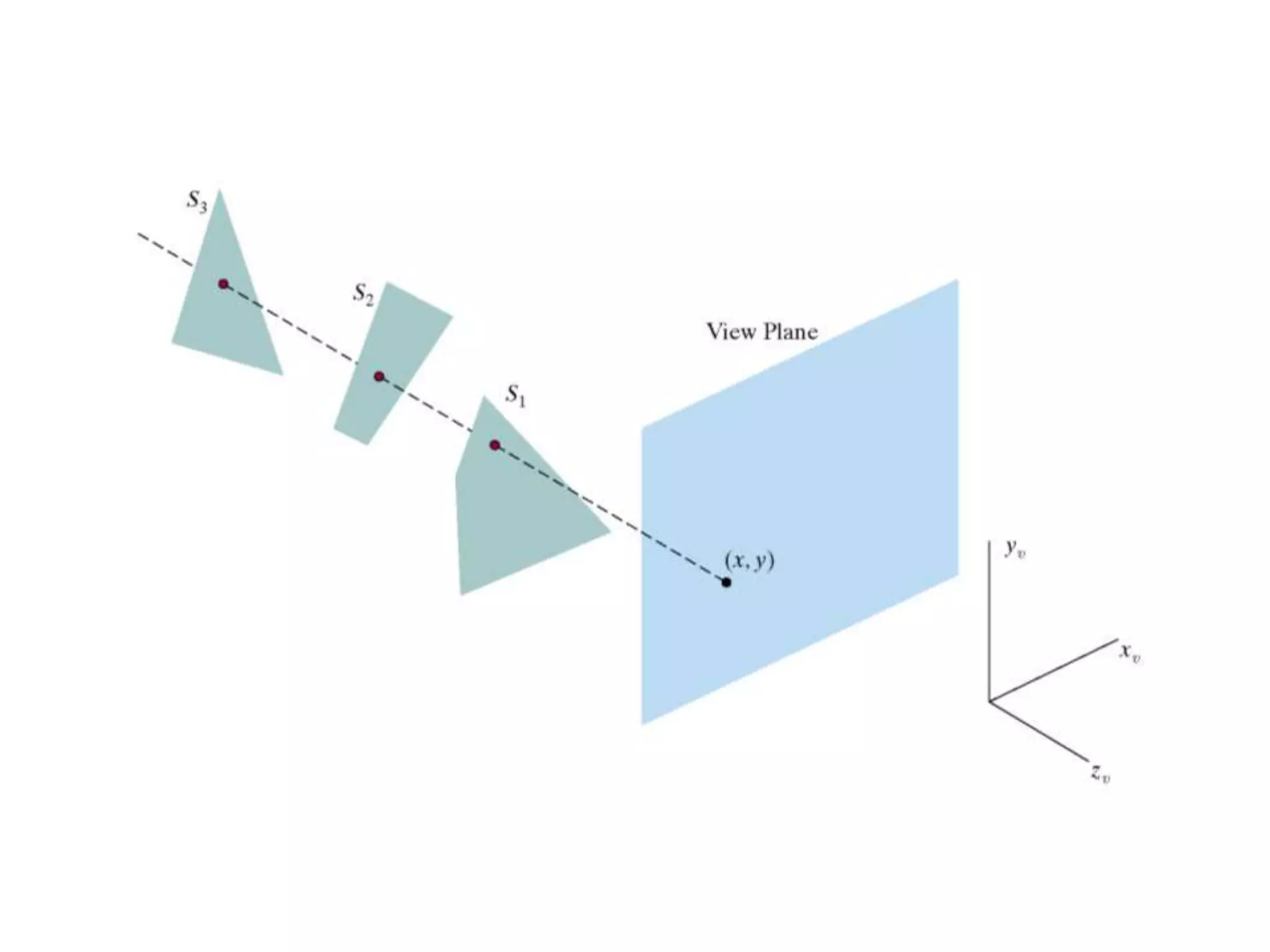
Presents the Z-buffer method for detecting visible surfaces, including buffer usage and depth comparison process.
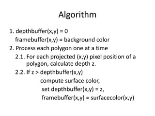
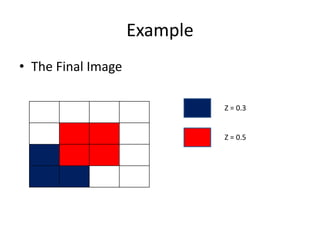
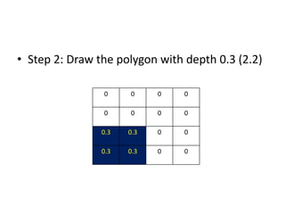
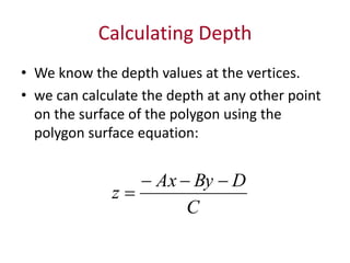
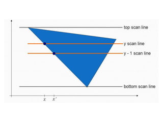
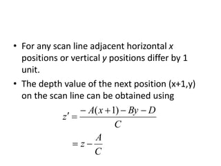
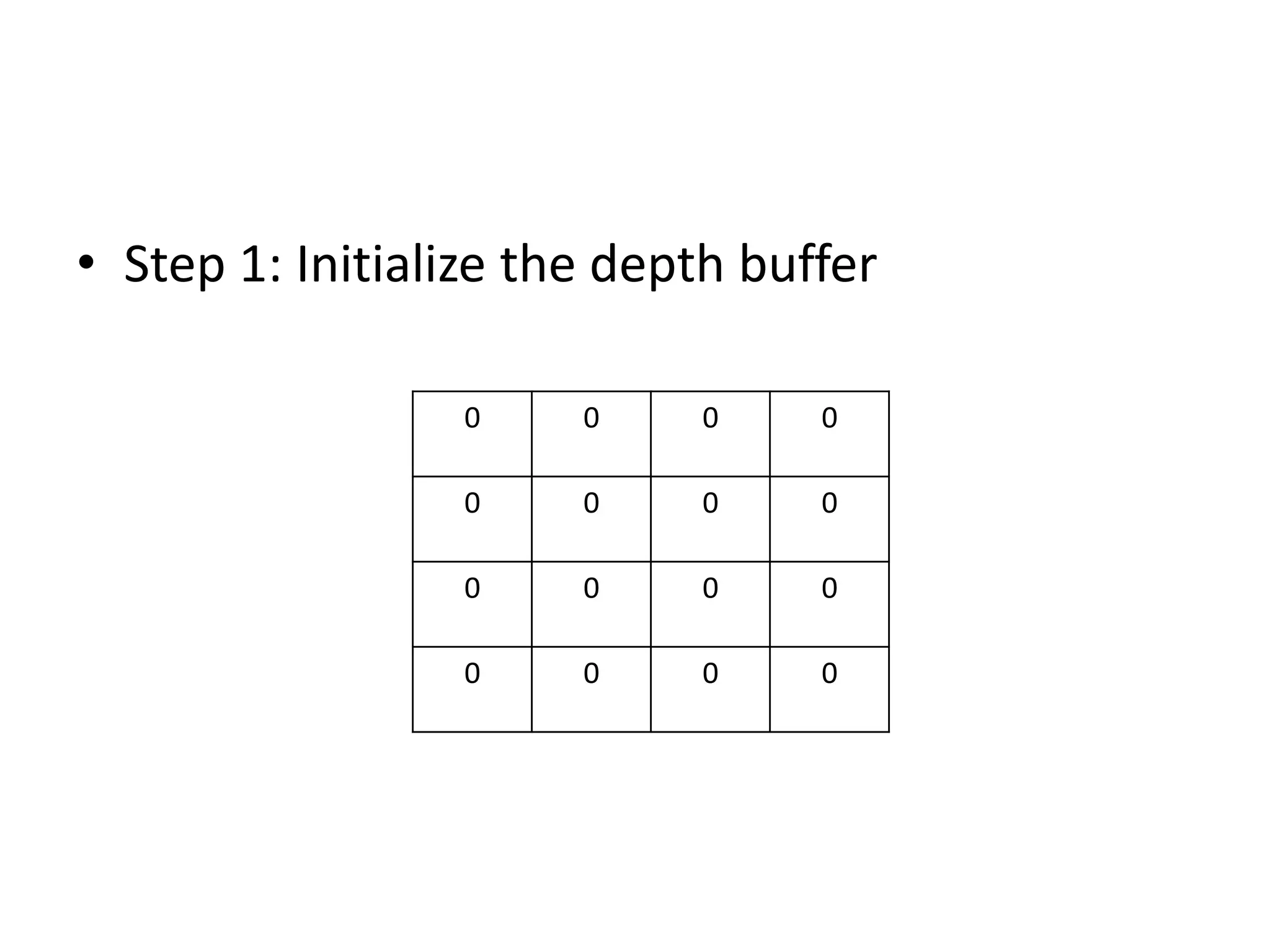
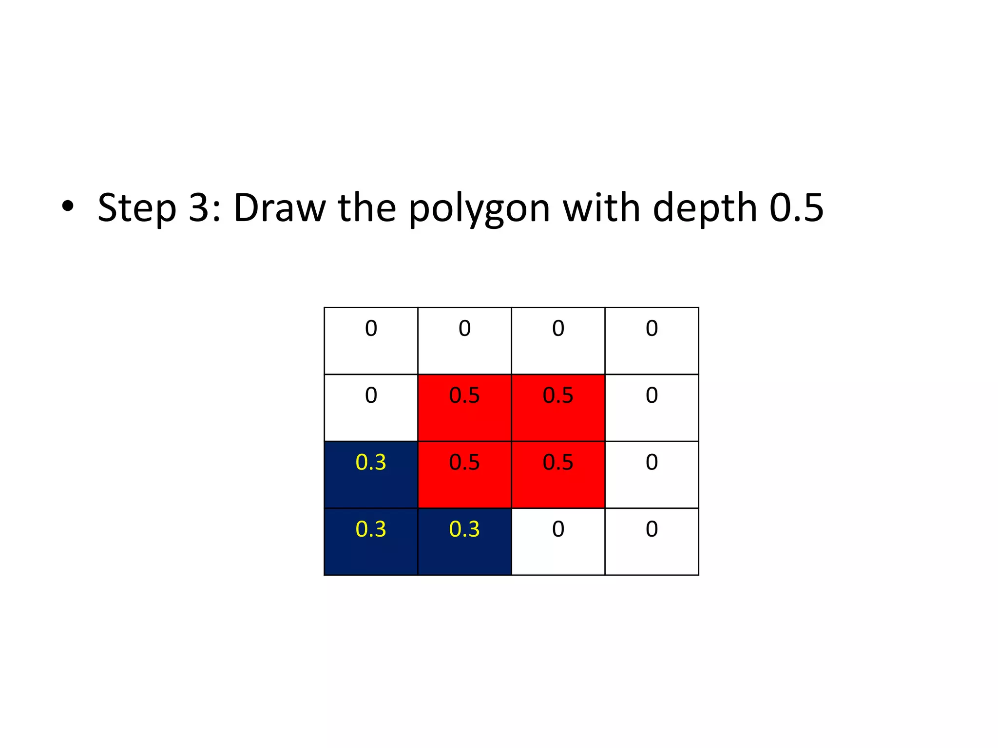
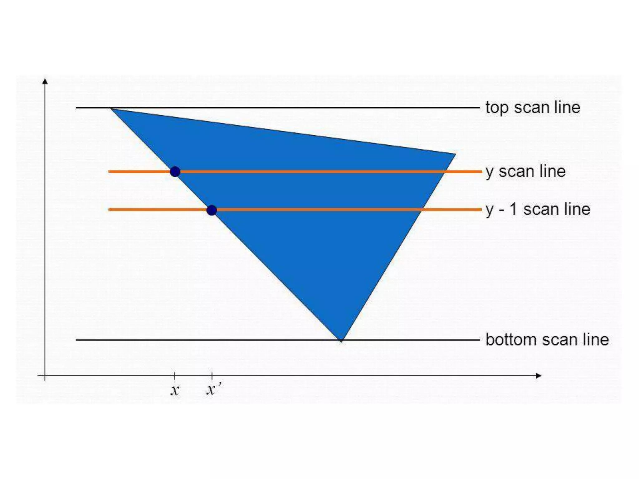
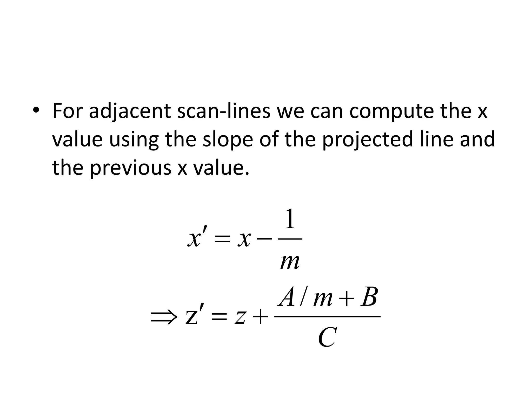
Step-by-step explanation of the depth-buffer algorithm for processing polygons and calculating depth values.
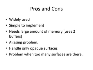
Pros and cons of the depth-buffer method focusing on its usage, memory needs, and limitations.
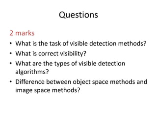
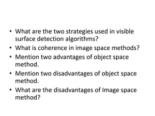
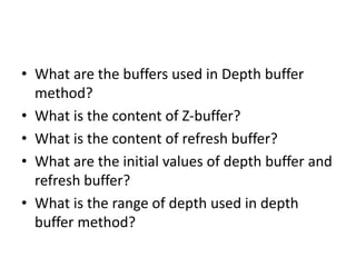
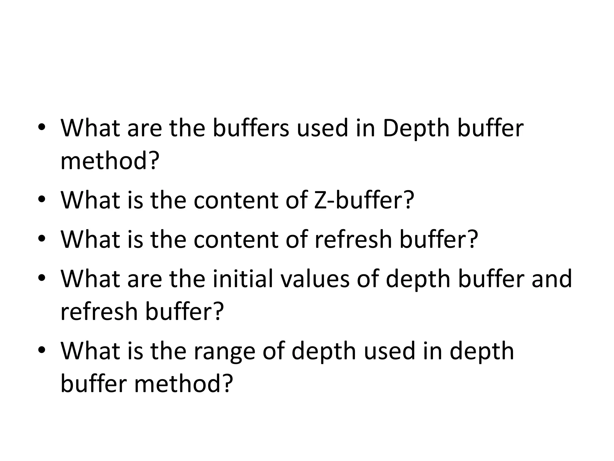
Questions reviewing key concepts from the presentation including visible detection methods and depth buffer specifics.
Ending quote encouraging resilience and a thank you to the audience for their attention.