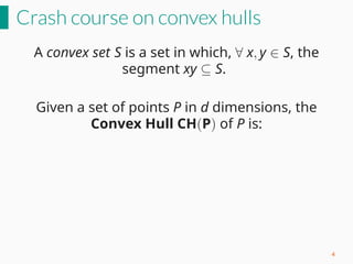
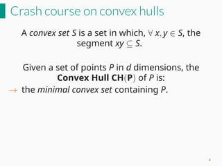
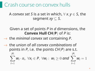
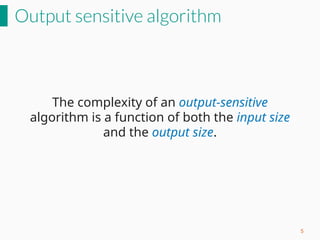
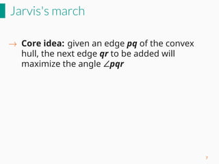
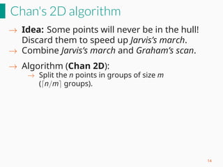
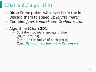
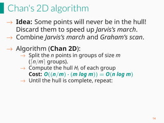
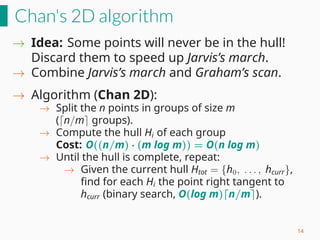
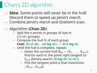
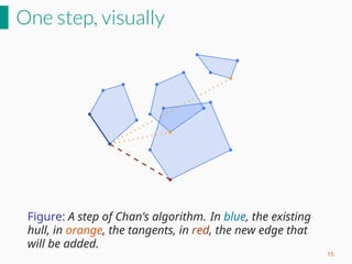
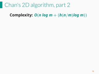
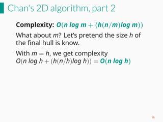
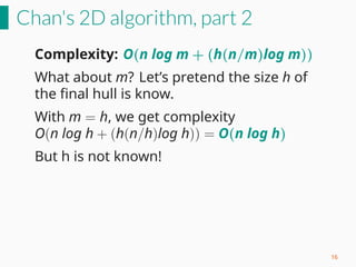
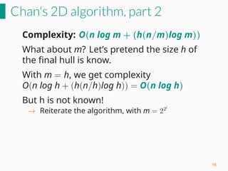
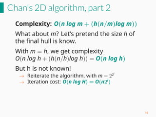
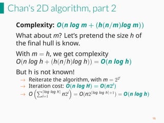
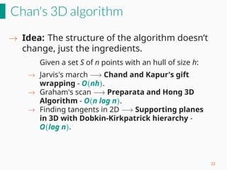
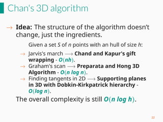
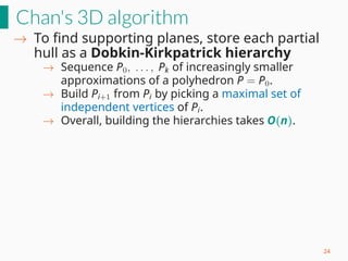
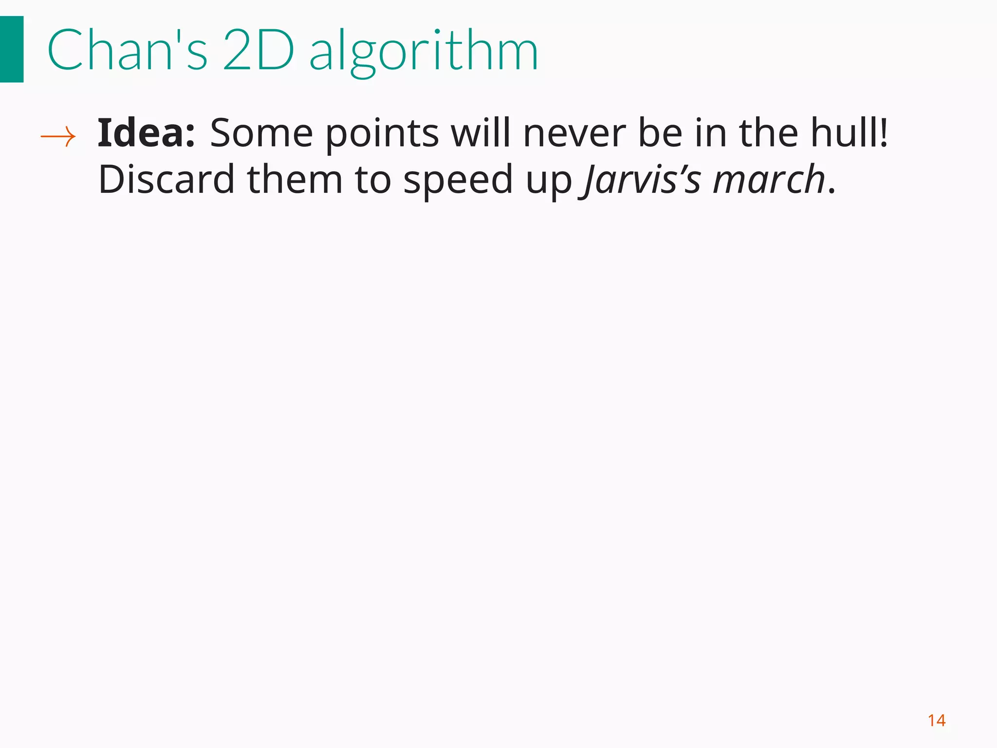
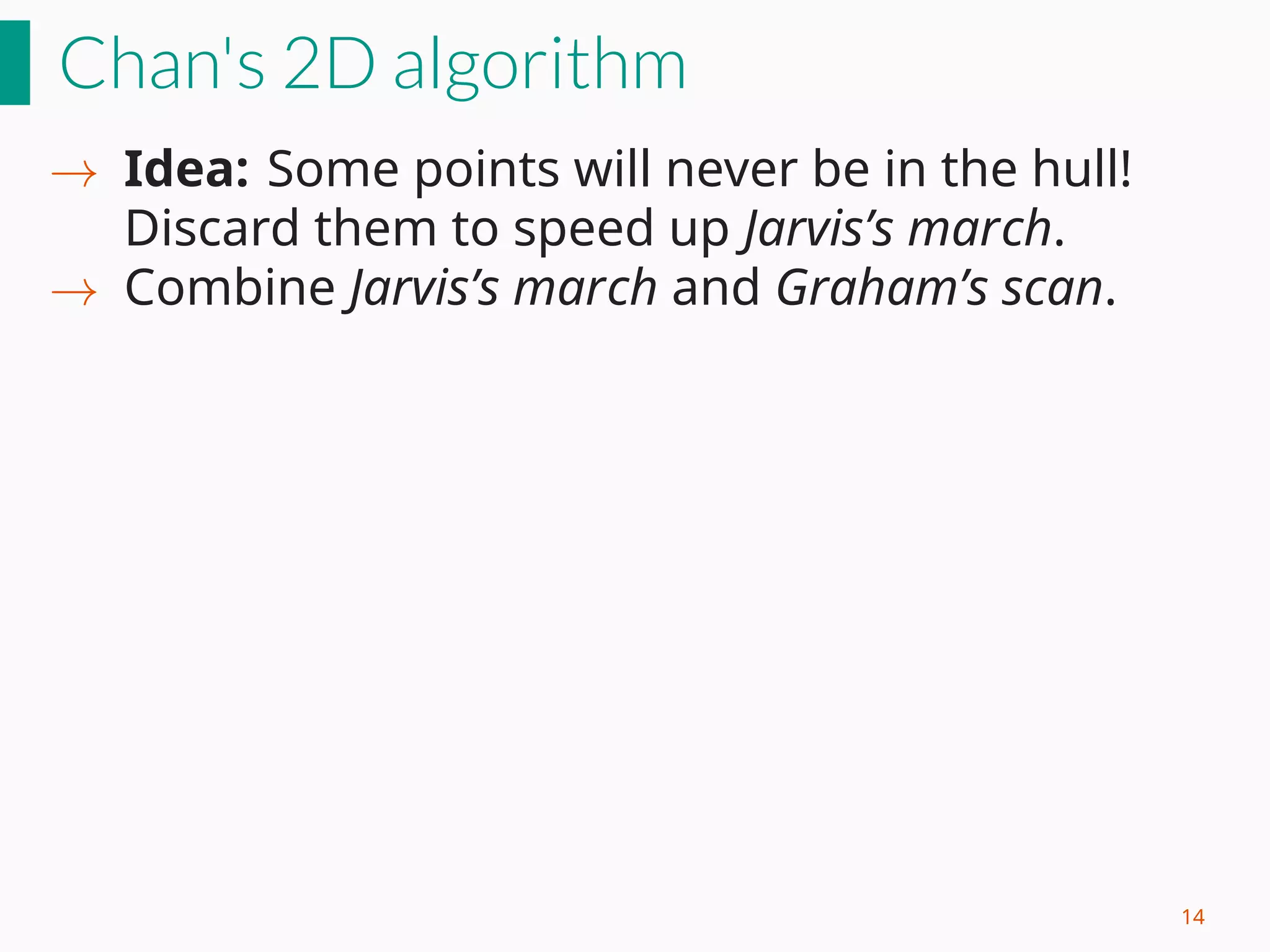
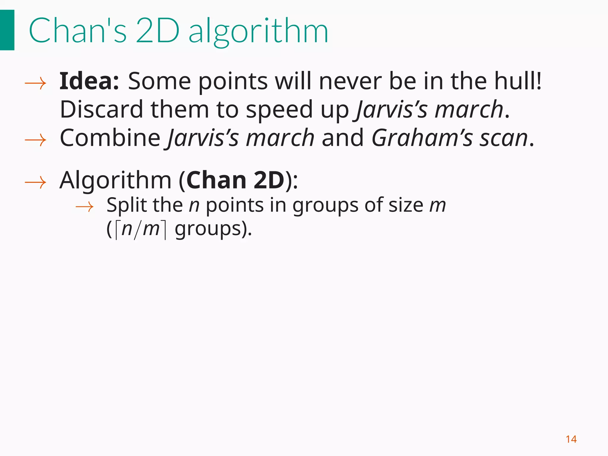
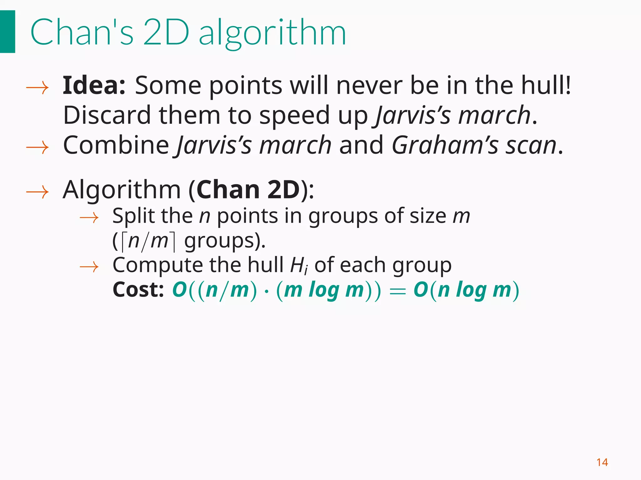
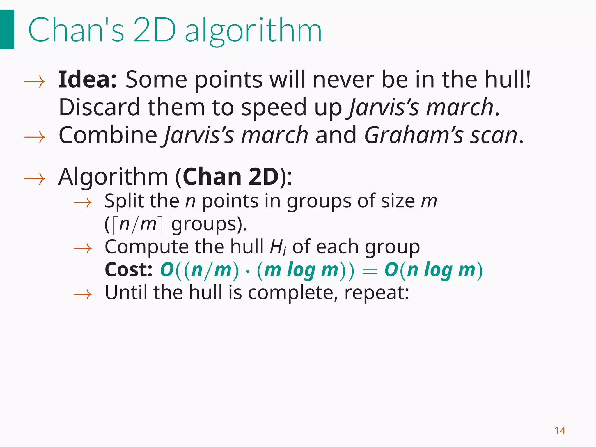
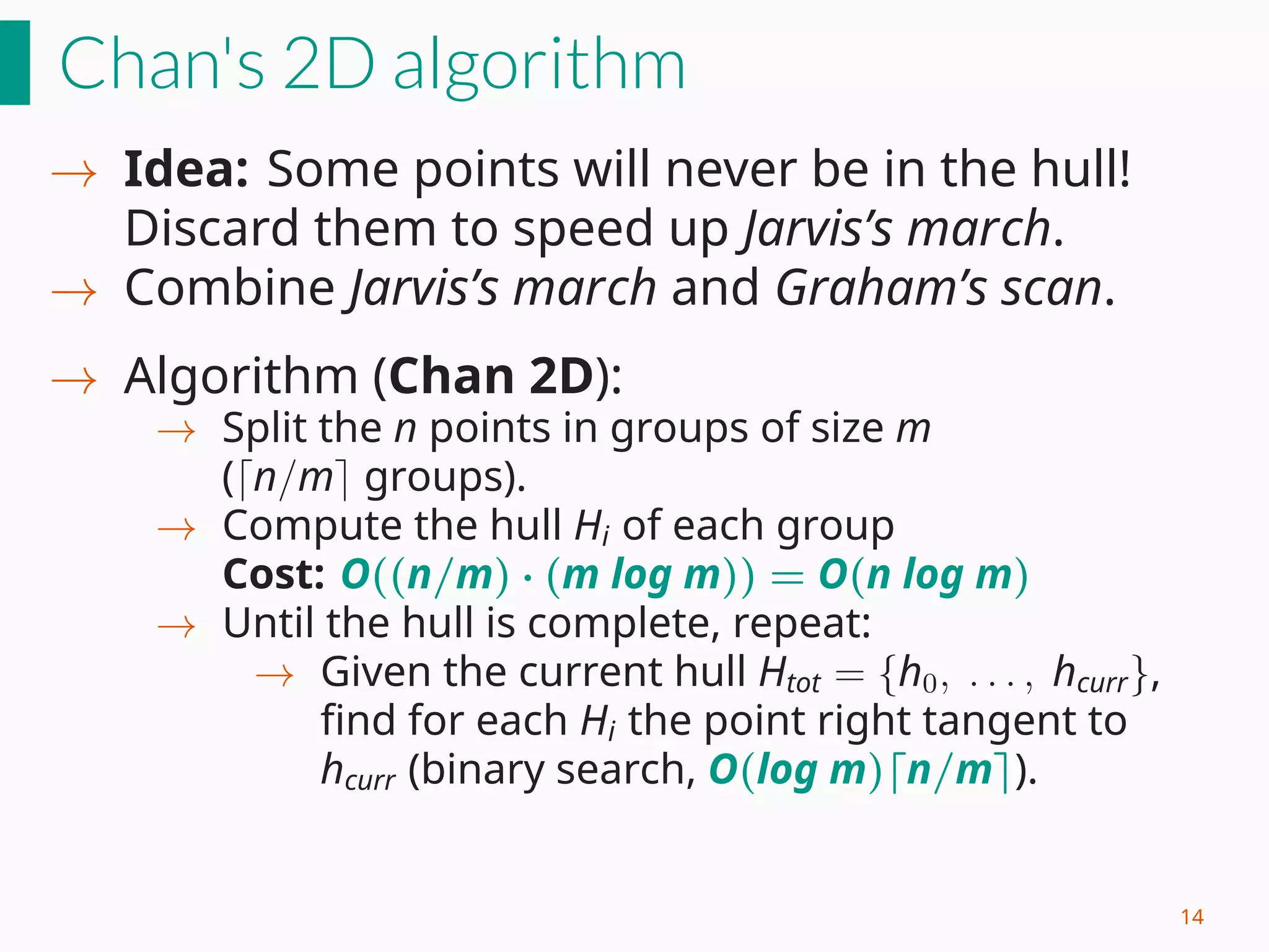
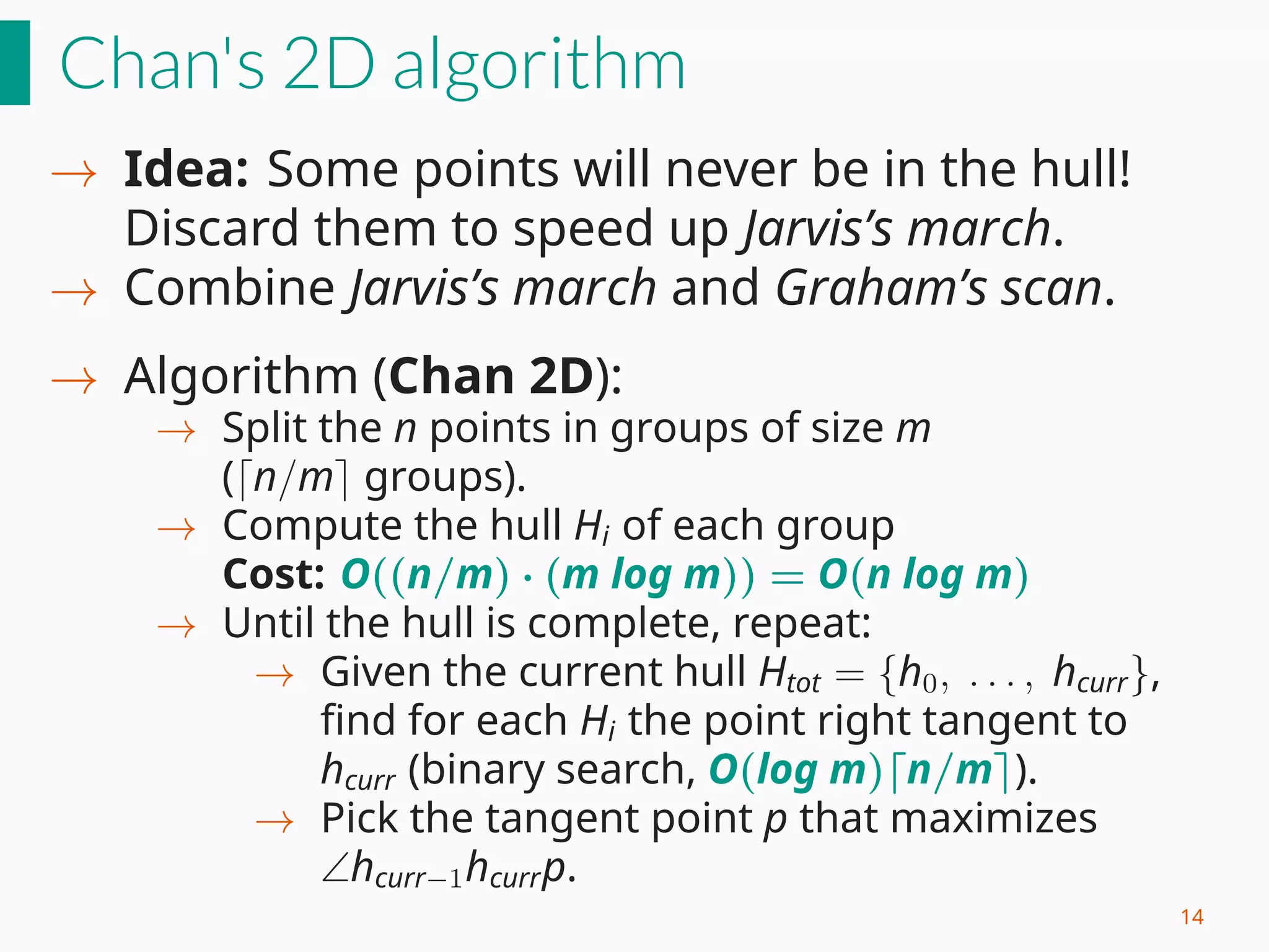
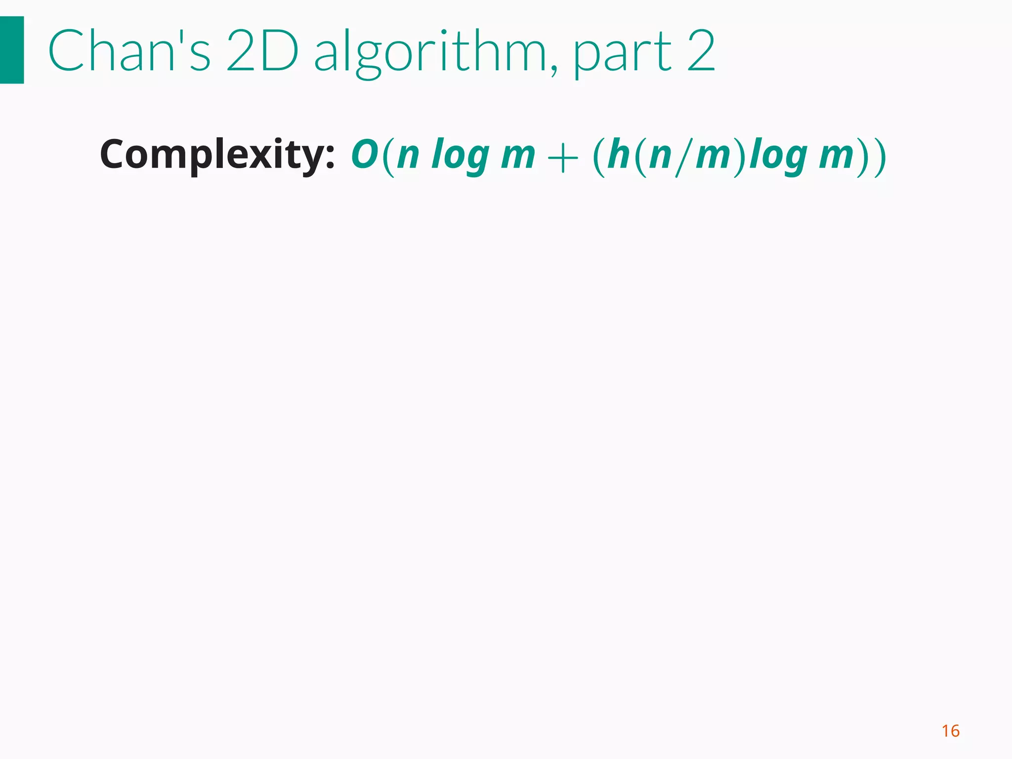
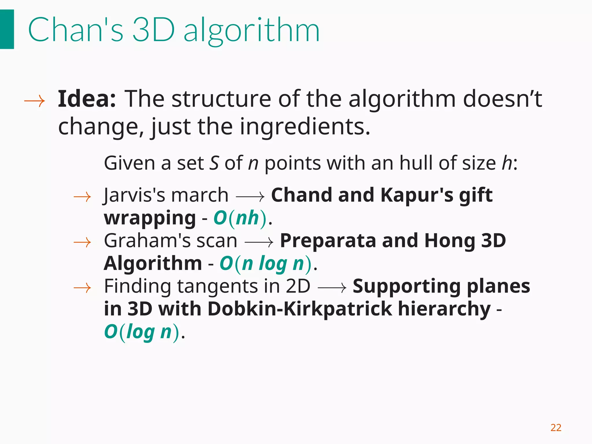
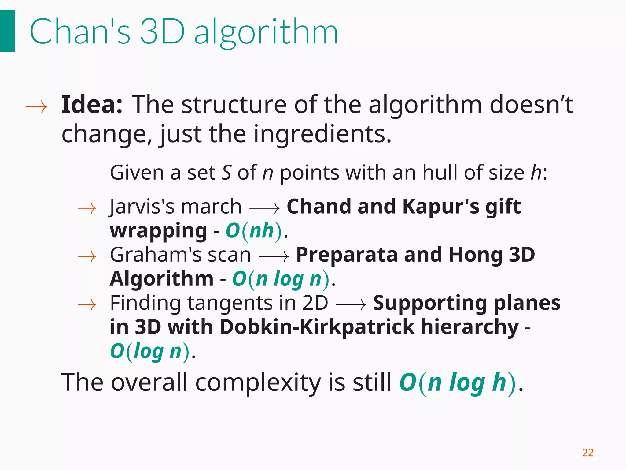
This document summarizes Chan's optimal output sensitive algorithms for computing convex hulls in 2D and 3D. It begins with basic notions of convex hulls, then describes Jarvis's march and Graham's scan algorithms for 2D convex hulls. It introduces Chan's 2D algorithm, which combines Jarvis's march and Graham's scan to achieve optimal O(n log h) time complexity, where h is the size of the hull. The document then explains how Chan extended this approach to 3D convex hulls by replacing the components with their 3D analogues, resulting in an optimal output sensitive 3D convex hull algorithm.


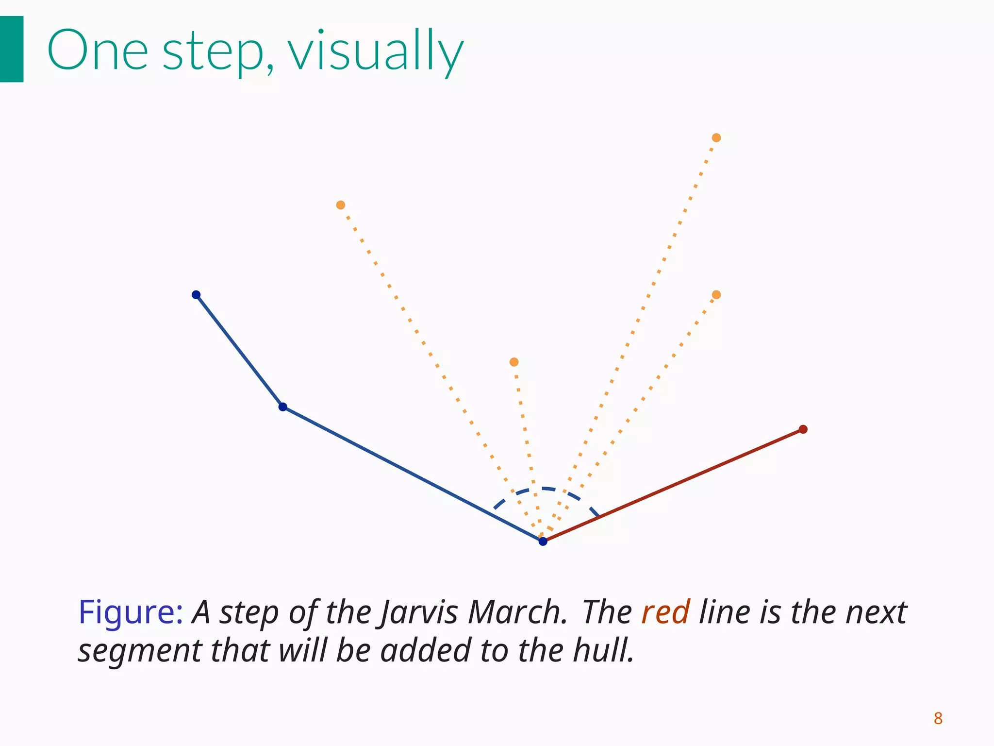
![Jarvis's march
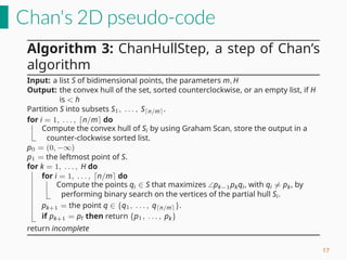
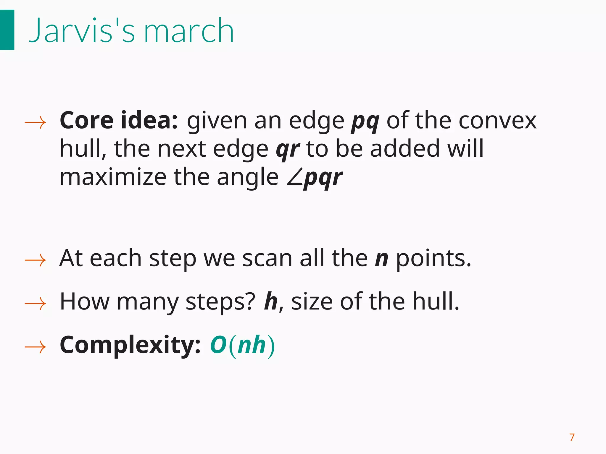
Algorithm 1: Jarvis March
Input: a list S of bidimensional points.
Output: the convex hull of the set, sorted counterclockwise.
hull =[]
x0 = the leftmost point.
hull.push(x0)
Loop hull.last() != hull.first()
candidate = S.first()
foreach p in S do
if p != hull.last() and p is on the right of the segment
”hull.last(), candidate” then
candidate = p
if candidate != hull.first then hull.push(candidate) else break
return hull
9](https://image.slidesharecdn.com/presentation-161214090546/85/Convex-hulls-Chan-s-algorithm-17-320.jpg)
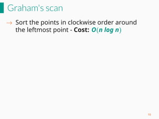
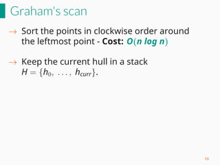
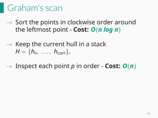
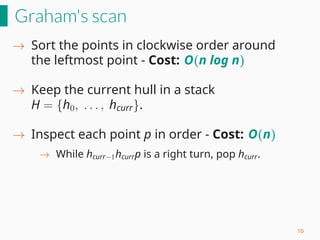
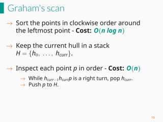
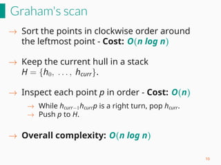
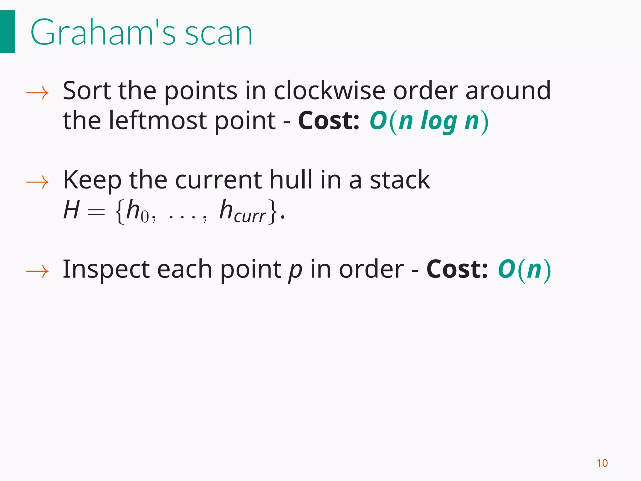
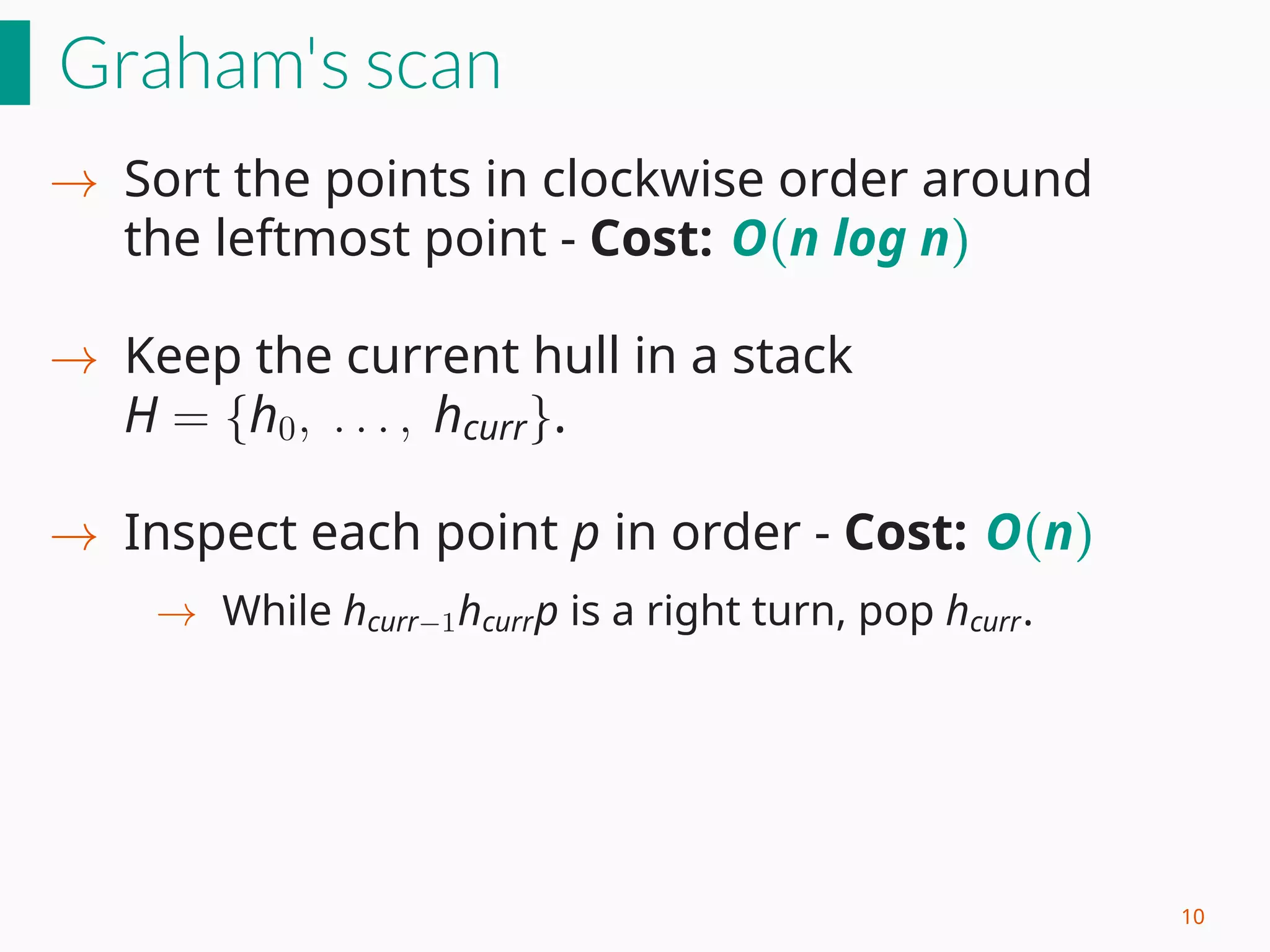
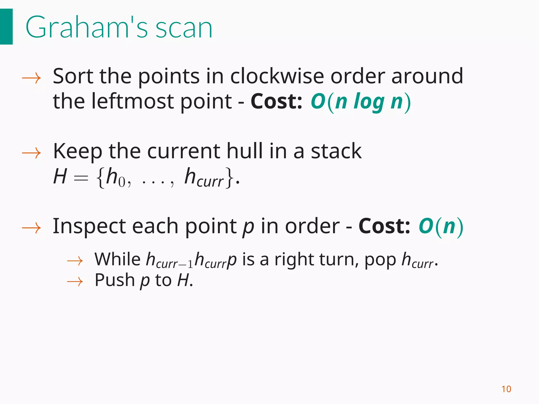
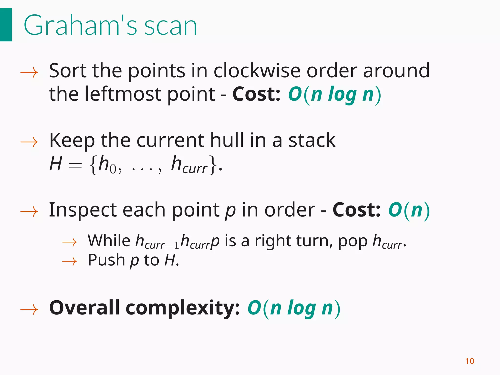
![Graham's scan
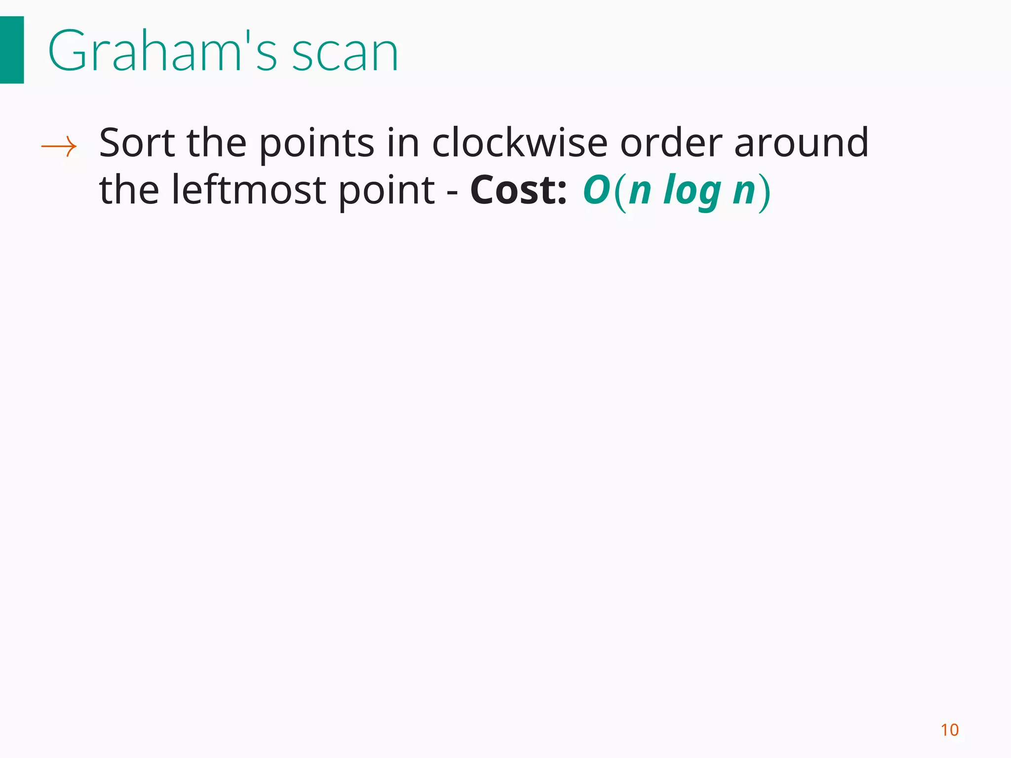
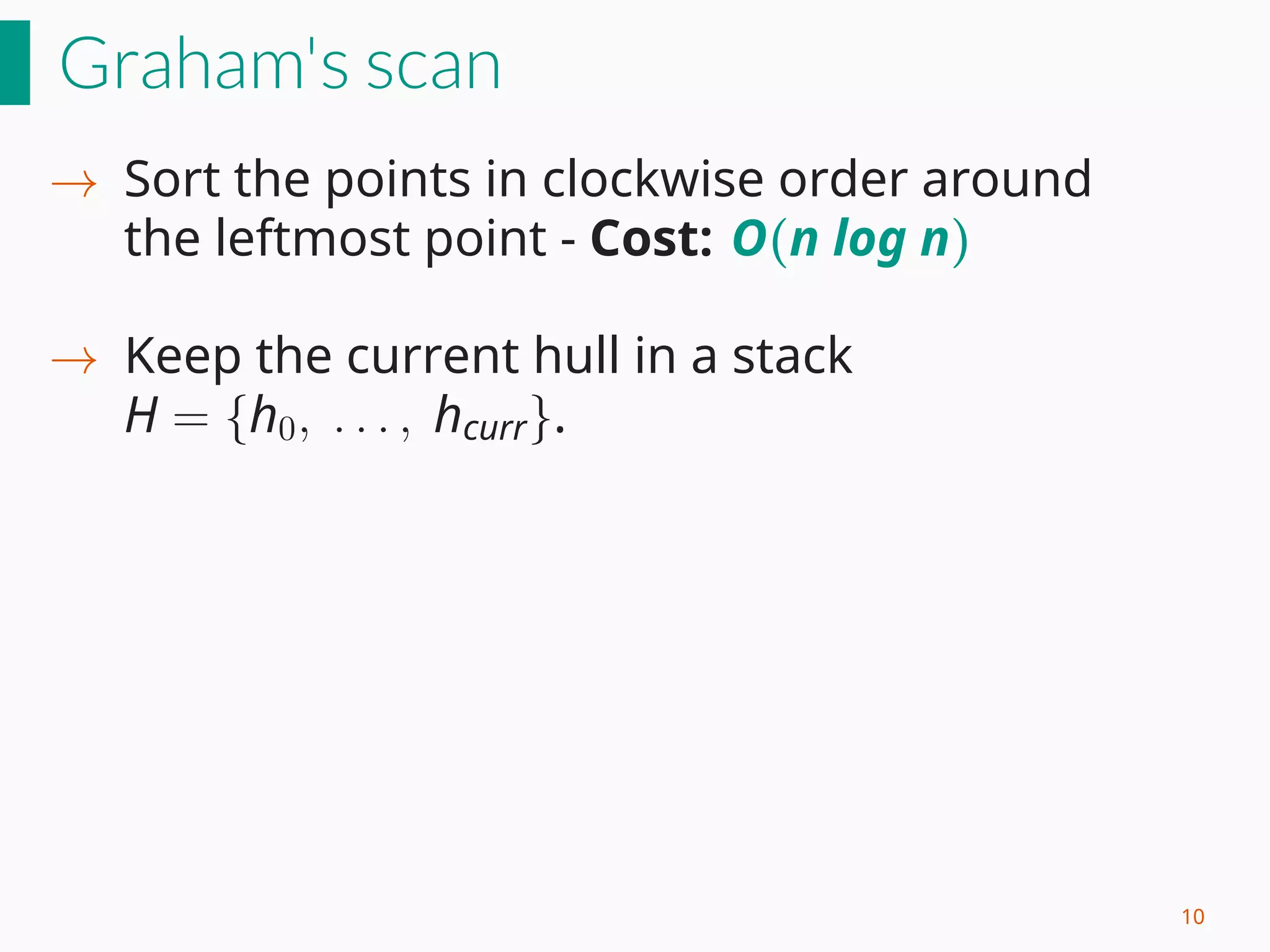
Algorithm 2: Graham Scan
Input: a list S of bidimensional points.
Output: the convex hull of the set, sorted counterclockwise.
hull =[]
x0 = the leftmost point.
Put x0 as the first element of S.
Sort the remaining points in counter-clockwise order, with
respect to x0.
Add the first 3 points in S to the hull.
forall the remaining points in S do
while hull.second_to_last(), hull.last(), p form a right turn do
hull.pop()
hull.push(p)
return hull
11](https://image.slidesharecdn.com/presentation-161214090546/85/Convex-hulls-Chan-s-algorithm-24-320.jpg)


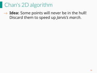


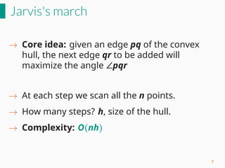
![Chan's 2D - Empirical analysis
Is a real implementation O(n log h)?
Test 1: fixed hull size (1000), increasing number of
points.
0
10
20
30
40
50
50000
100000
150000
200000
Number of Points
Executiontime[sec]
Linear Model Real Data
19](https://image.slidesharecdn.com/presentation-161214090546/85/Convex-hulls-Chan-s-algorithm-49-320.jpg)
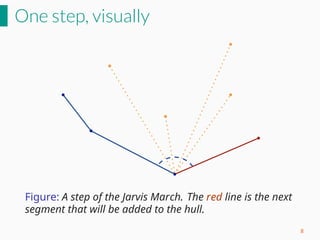
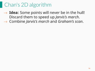
![Chan's 2D - Empirical analysis
Is a real implementation O(n log h)?
Test 2: fixed number of points (40000), increasing
hull size.
8
9
10
11 5000
10000
15000
20000
Size of the Hull
Executiontime[sec]
Logarithmic Model Real Data
20](https://image.slidesharecdn.com/presentation-161214090546/85/Convex-hulls-Chan-s-algorithm-50-320.jpg)


![References I
[1] C. Bradford Barber, David P. Dobkin, and Huhdanpaa Hannu.
The quickhull algorithm for convex hulls.
1995.
[2] T. M. Chan.
Optimal output-sensitive convex hull algorithms in two and three
dimensions.
Discrete & Computational Geometry, 16(4):361–368, 1996.
[3] Donald R. Chand and Sham S. Kapur.
[4] Ioannis Z. Emiris and John F. Canny.
An efficient approach to removing geometric degeneracies.
Technical report, 1991.
[5] Christer Ericson.
Real-Time Collision Detection.
CRC Press, Inc., Boca Raton, FL, USA, 2004.
[6] A. Goshtasby and G. C. Stockman.
Point pattern matching using convex hull edges.
IEEE Transactions on Systems, Man, and Cybernetics, SMC-15(5), 1985.
26](https://image.slidesharecdn.com/presentation-161214090546/85/Convex-hulls-Chan-s-algorithm-76-320.jpg)
![References II
[7] David G. Kirkpatrick and Raimund Seidel.
The ultimate planar convex hull algorithm ?
Technical report, 1983.
[8] Joseph O’Rourke.
Computational Geometry in C.
Cambridge University Press, 2nd edition, 1998.
[9] F. P. Preparata and S. J. Hong.
Convex hulls of finite sets of points in two and three dimensions.
Commun. ACM, 20(2):87–93, February 1977.
[10] Franco P. Preparata and Michael I. Shamos.
Computational Geometry: An Introduction.
Springer-Verlag New York, Inc., 1985.
[11] Franco P. Preparata and Michael I. Shamos.
Computational Geometry: An Introduction.
Springer-Verlag New York, Inc., 1985.
Beamer theme: Presento, by Ratul Saha. The research system in Germany, by
Hazem Alsaied
27](https://image.slidesharecdn.com/presentation-161214090546/85/Convex-hulls-Chan-s-algorithm-77-320.jpg)


![Jarvis's march
Algorithm 1: Jarvis March
Input: a list S of bidimensional points.
Output: the convex hull of the set, sorted counterclockwise.
hull =[]
x0 = the leftmost point.
hull.push(x0)
Loop hull.last() != hull.first()
candidate = S.first()
foreach p in S do
if p != hull.last() and p is on the right of the segment
”hull.last(), candidate” then
candidate = p
if candidate != hull.first then hull.push(candidate) else break
return hull
9](https://image.slidesharecdn.com/presentation-161214090546/75/Convex-hulls-Chan-s-algorithm-17-2048.jpg)
![Graham's scan
Algorithm 2: Graham Scan
Input: a list S of bidimensional points.
Output: the convex hull of the set, sorted counterclockwise.
hull =[]
x0 = the leftmost point.
Put x0 as the first element of S.
Sort the remaining points in counter-clockwise order, with
respect to x0.
Add the first 3 points in S to the hull.
forall the remaining points in S do
while hull.second_to_last(), hull.last(), p form a right turn do
hull.pop()
hull.push(p)
return hull
11](https://image.slidesharecdn.com/presentation-161214090546/75/Convex-hulls-Chan-s-algorithm-24-2048.jpg)


![Chan's 2D - Empirical analysis
Is a real implementation O(n log h)?
Test 1: fixed hull size (1000), increasing number of
points.
0
10
20
30
40
50
50000
100000
150000
200000
Number of Points
Executiontime[sec]
Linear Model Real Data
19](https://image.slidesharecdn.com/presentation-161214090546/75/Convex-hulls-Chan-s-algorithm-49-2048.jpg)
![Chan's 2D - Empirical analysis
Is a real implementation O(n log h)?
Test 2: fixed number of points (40000), increasing
hull size.
8
9
10
11 5000
10000
15000
20000
Size of the Hull
Executiontime[sec]
Logarithmic Model Real Data
20](https://image.slidesharecdn.com/presentation-161214090546/75/Convex-hulls-Chan-s-algorithm-50-2048.jpg)


![References I
[1] C. Bradford Barber, David P. Dobkin, and Huhdanpaa Hannu.
The quickhull algorithm for convex hulls.
1995.
[2] T. M. Chan.
Optimal output-sensitive convex hull algorithms in two and three
dimensions.
Discrete & Computational Geometry, 16(4):361–368, 1996.
[3] Donald R. Chand and Sham S. Kapur.
[4] Ioannis Z. Emiris and John F. Canny.
An efficient approach to removing geometric degeneracies.
Technical report, 1991.
[5] Christer Ericson.
Real-Time Collision Detection.
CRC Press, Inc., Boca Raton, FL, USA, 2004.
[6] A. Goshtasby and G. C. Stockman.
Point pattern matching using convex hull edges.
IEEE Transactions on Systems, Man, and Cybernetics, SMC-15(5), 1985.
26](https://image.slidesharecdn.com/presentation-161214090546/75/Convex-hulls-Chan-s-algorithm-76-2048.jpg)
![References II
[7] David G. Kirkpatrick and Raimund Seidel.
The ultimate planar convex hull algorithm ?
Technical report, 1983.
[8] Joseph O’Rourke.
Computational Geometry in C.
Cambridge University Press, 2nd edition, 1998.
[9] F. P. Preparata and S. J. Hong.
Convex hulls of finite sets of points in two and three dimensions.
Commun. ACM, 20(2):87–93, February 1977.
[10] Franco P. Preparata and Michael I. Shamos.
Computational Geometry: An Introduction.
Springer-Verlag New York, Inc., 1985.
[11] Franco P. Preparata and Michael I. Shamos.
Computational Geometry: An Introduction.
Springer-Verlag New York, Inc., 1985.
Beamer theme: Presento, by Ratul Saha. The research system in Germany, by
Hazem Alsaied
27](https://image.slidesharecdn.com/presentation-161214090546/75/Convex-hulls-Chan-s-algorithm-77-2048.jpg)


