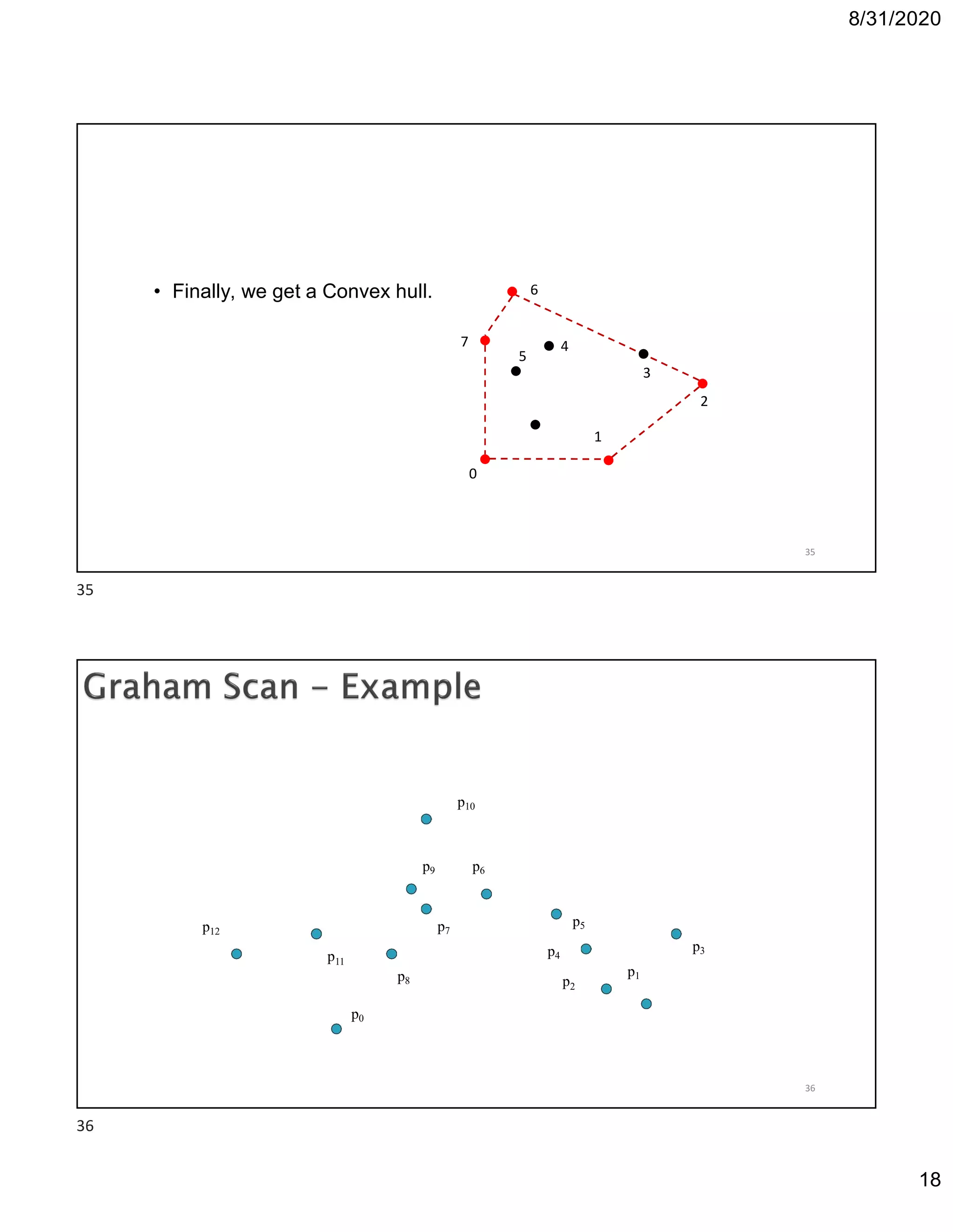
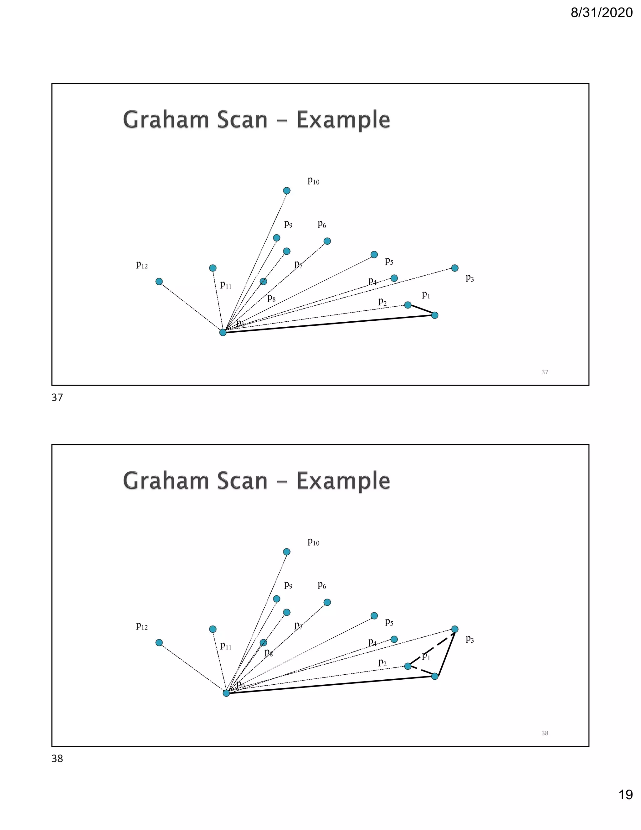
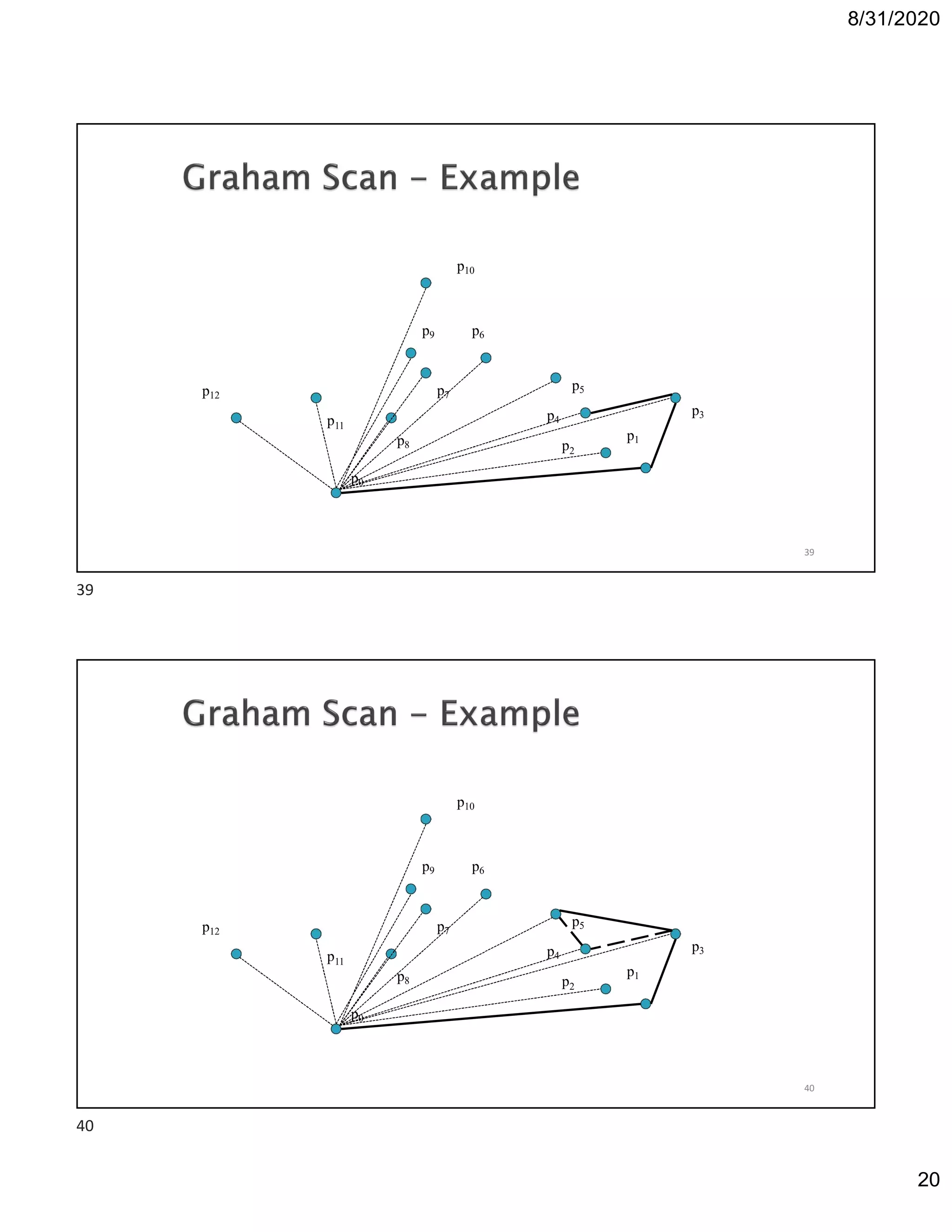
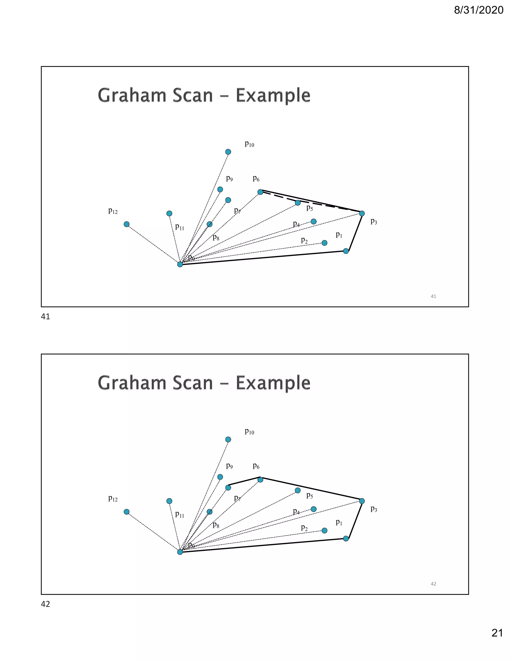
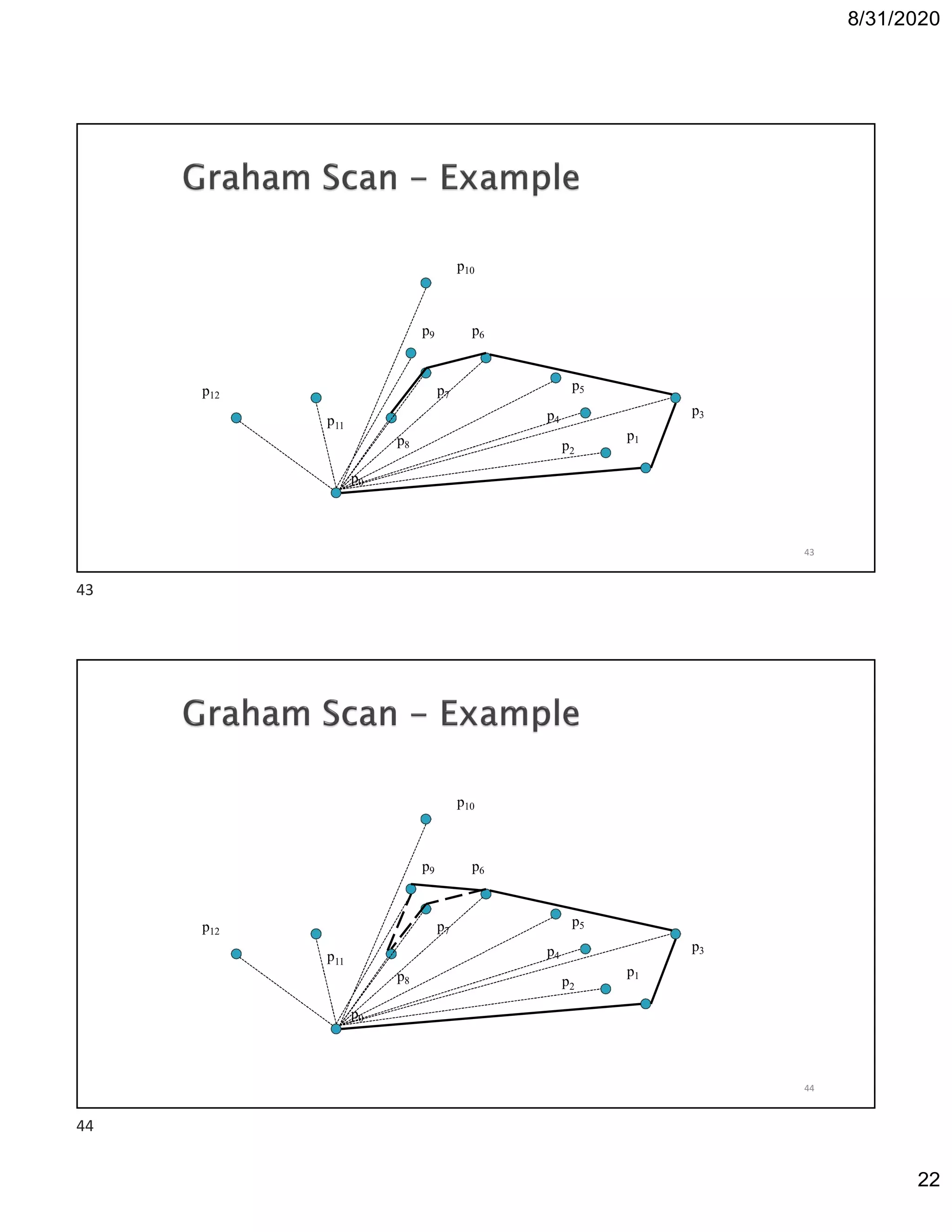
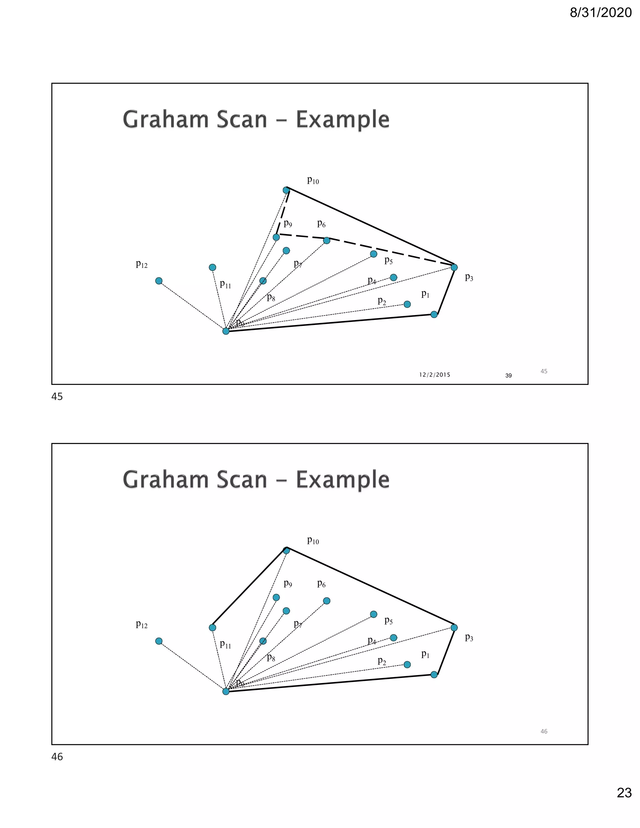
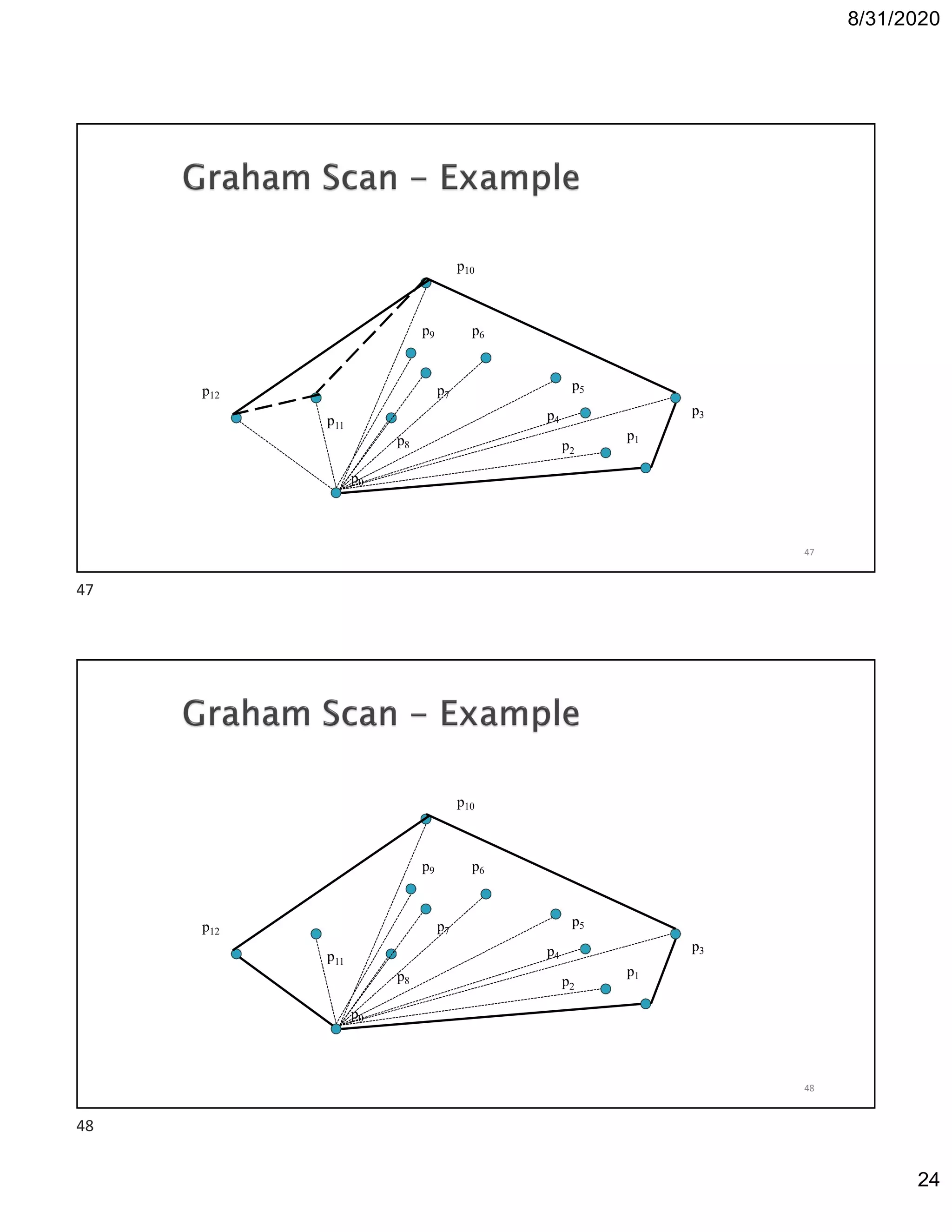
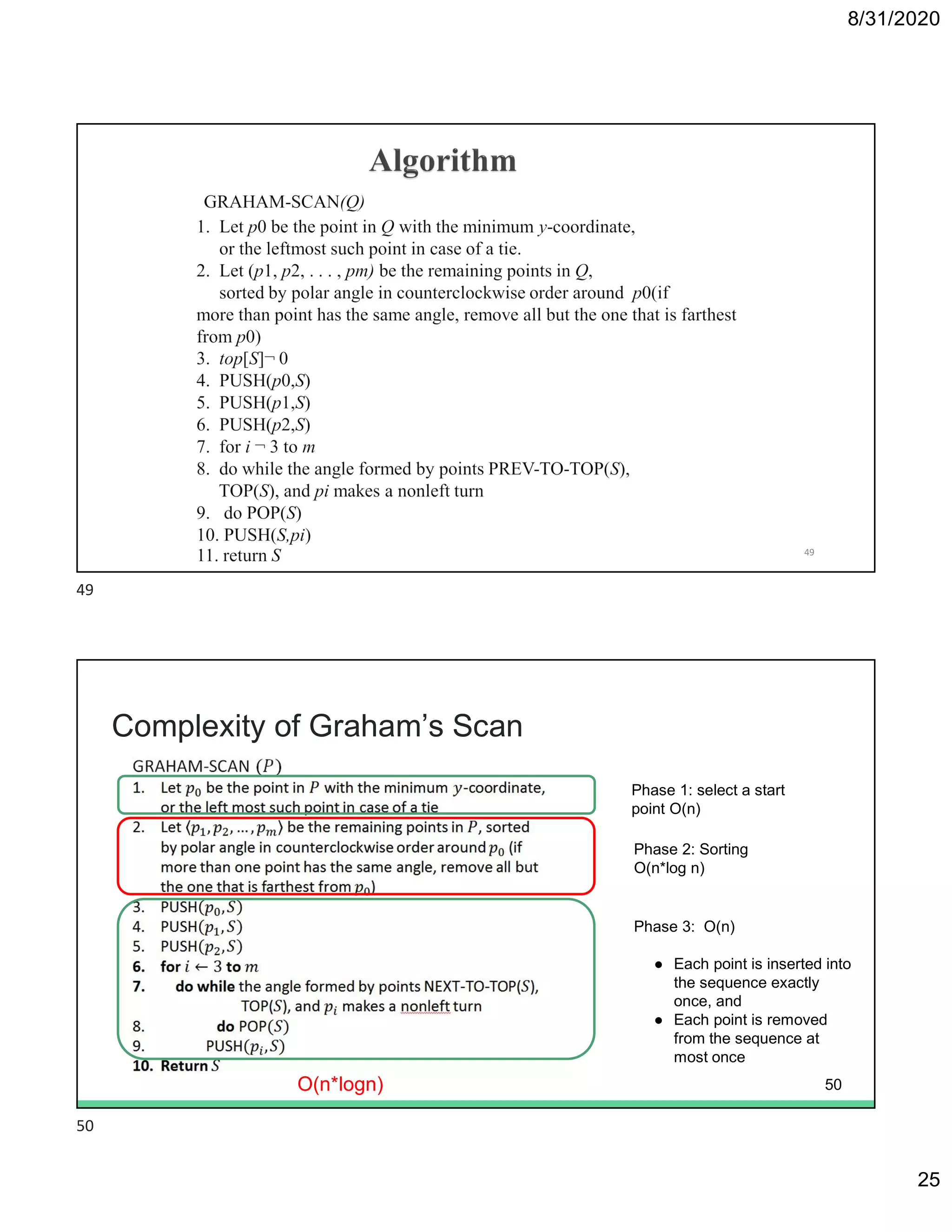
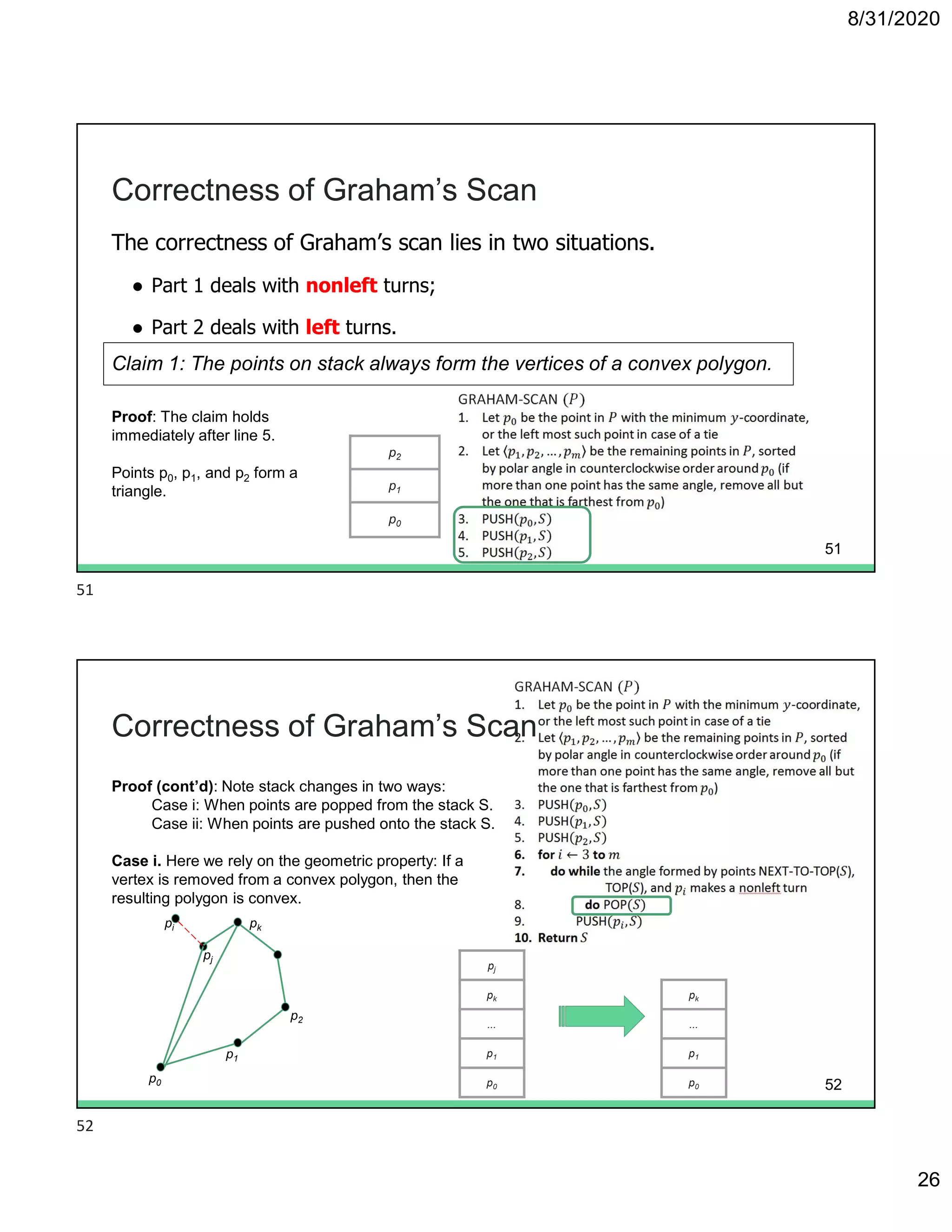
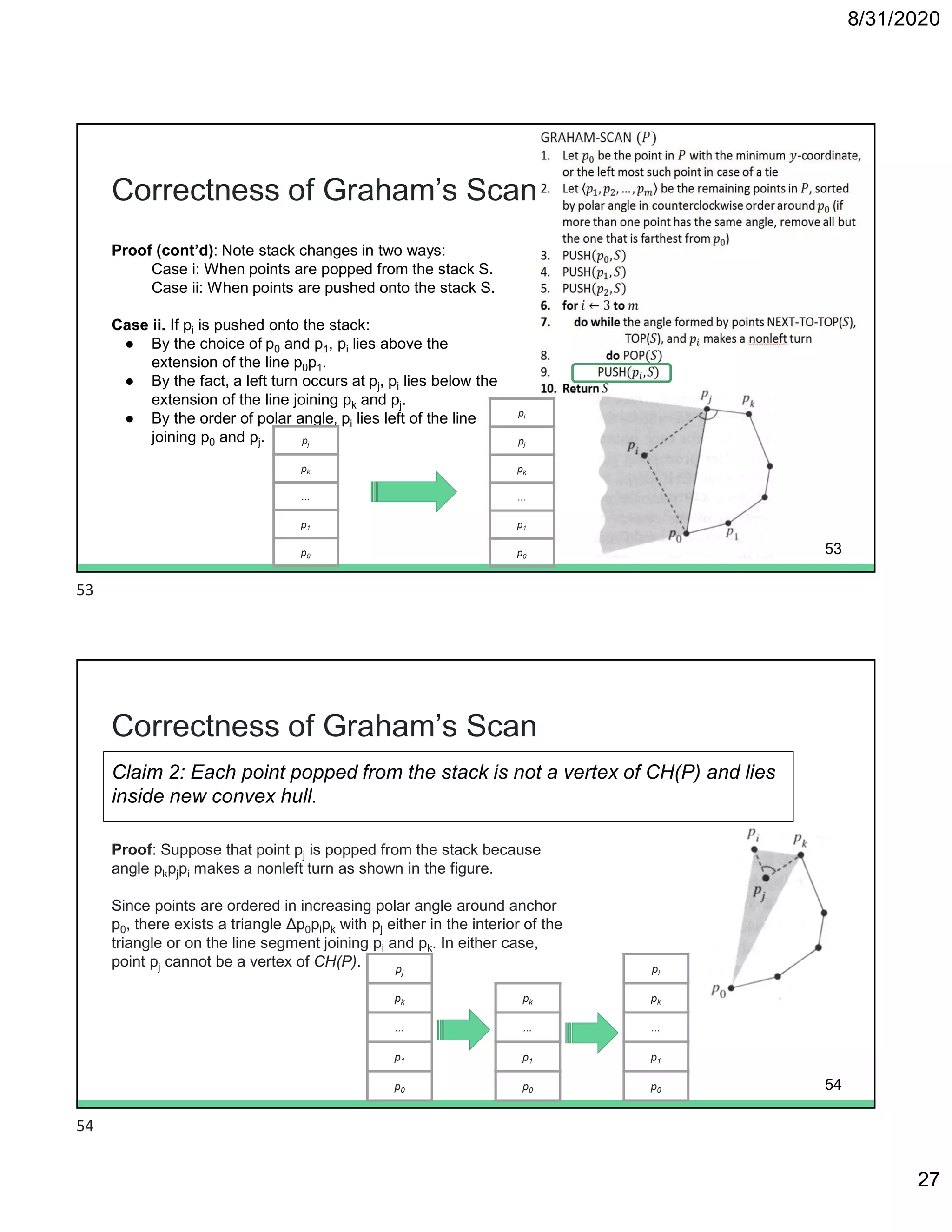
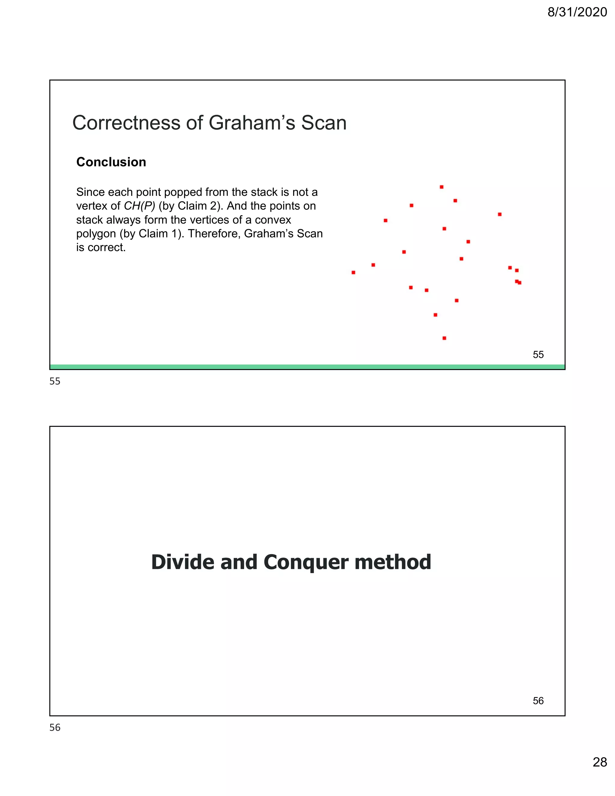
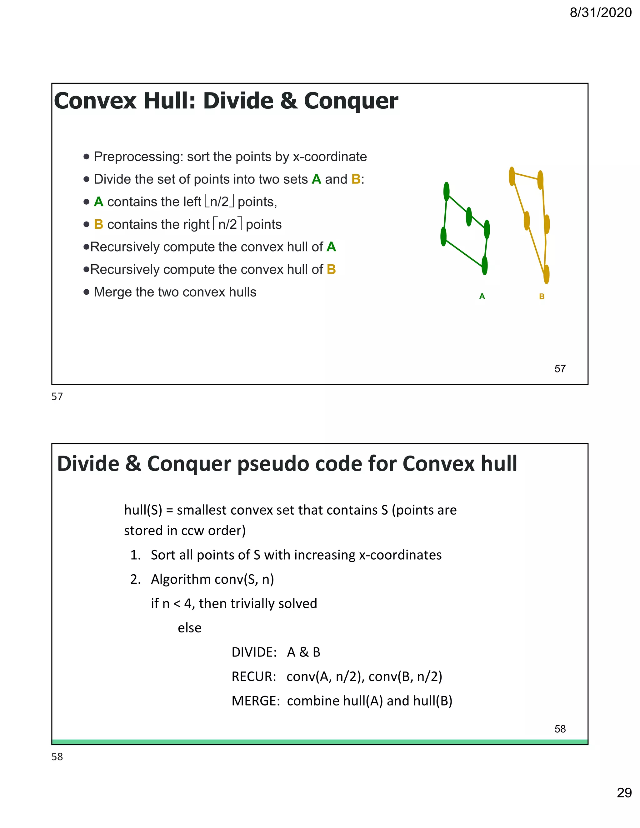
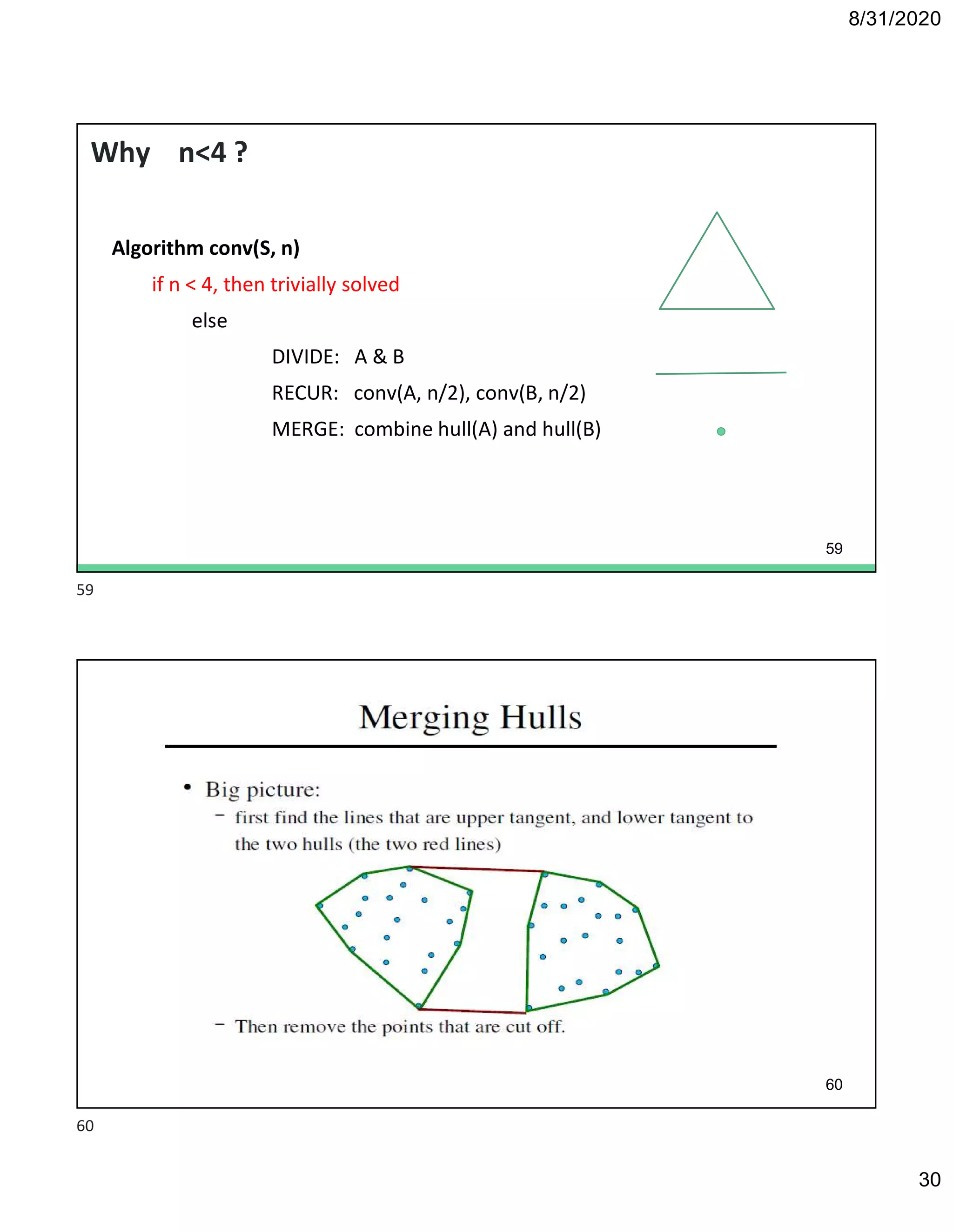
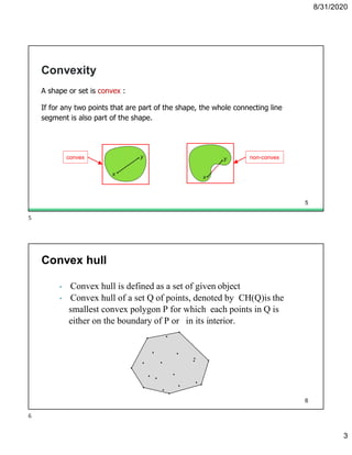
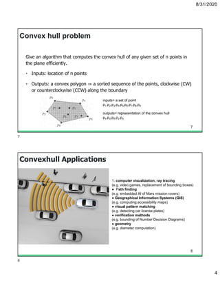
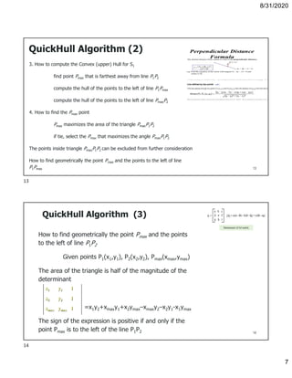
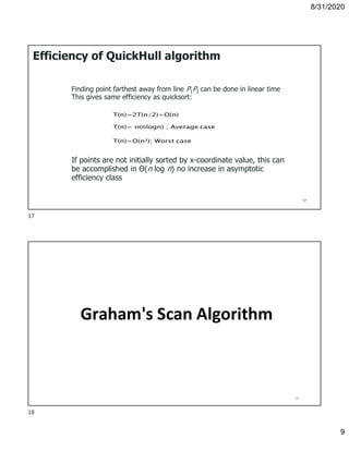
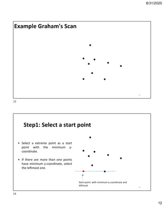
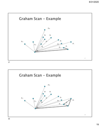
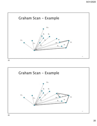
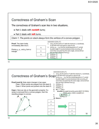
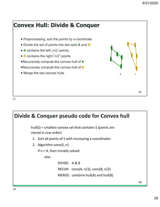
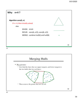
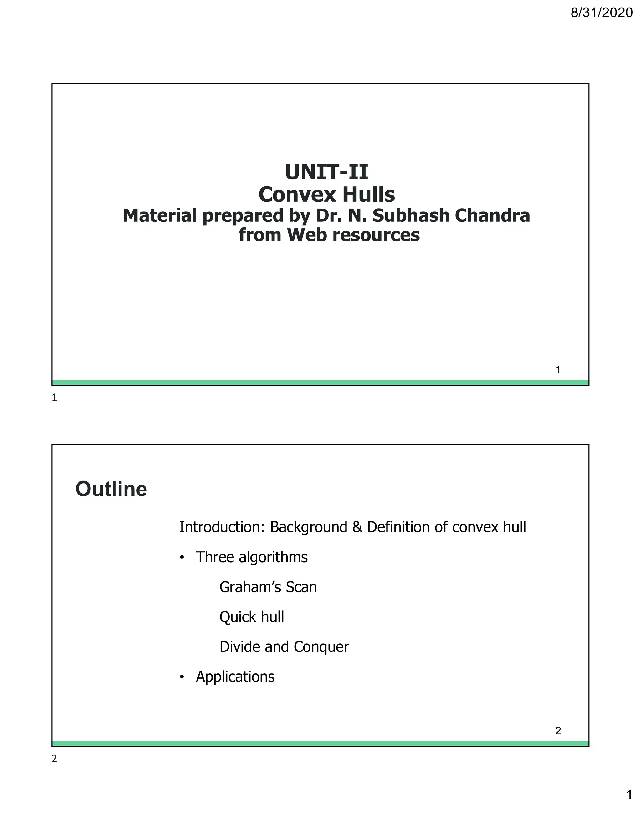
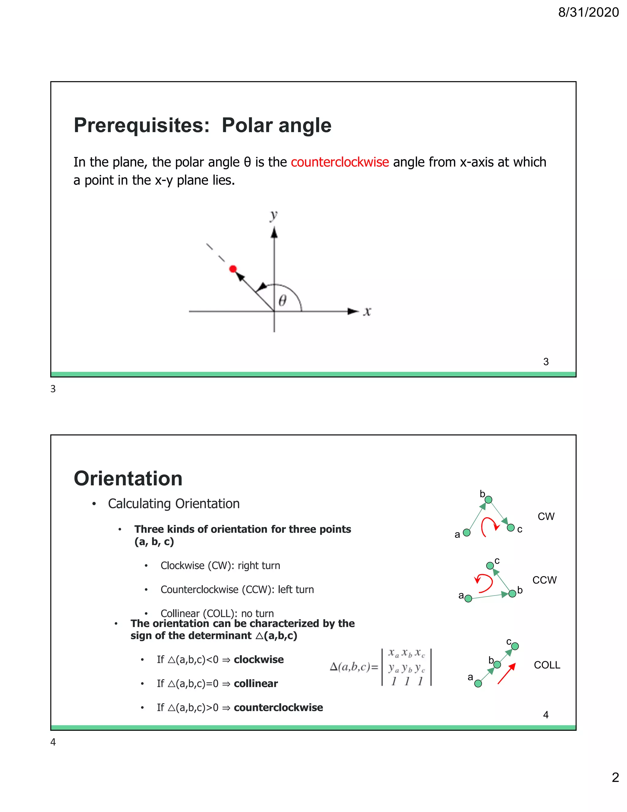
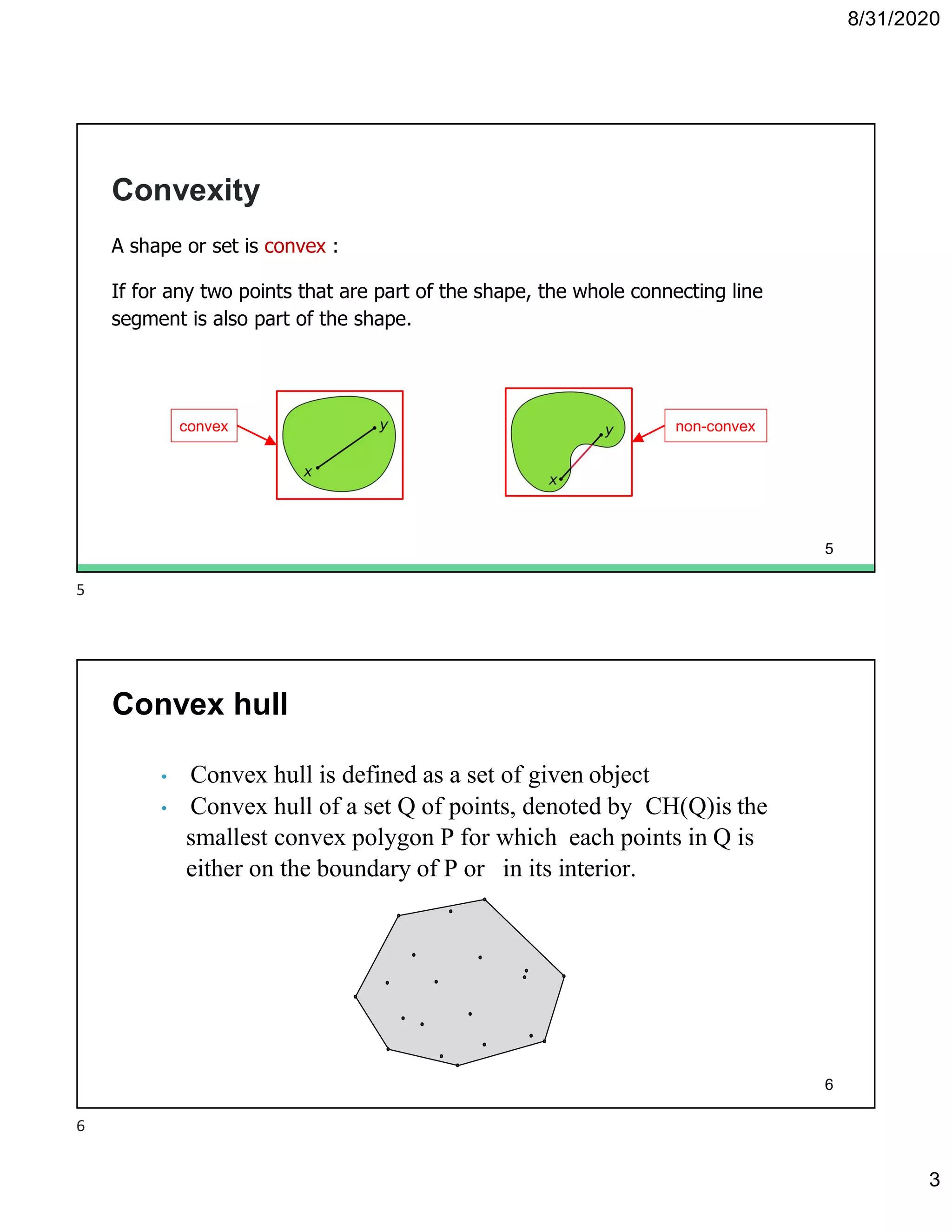
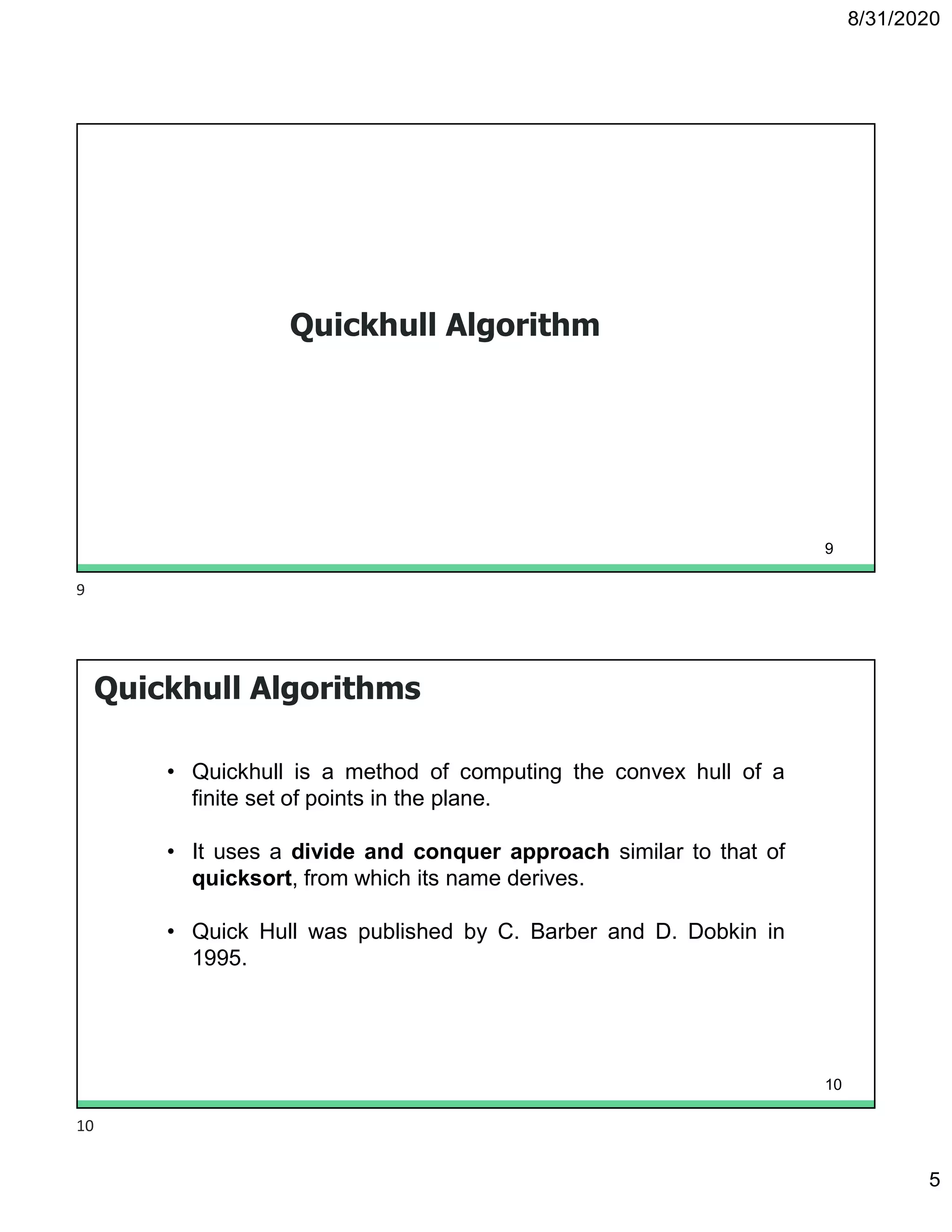
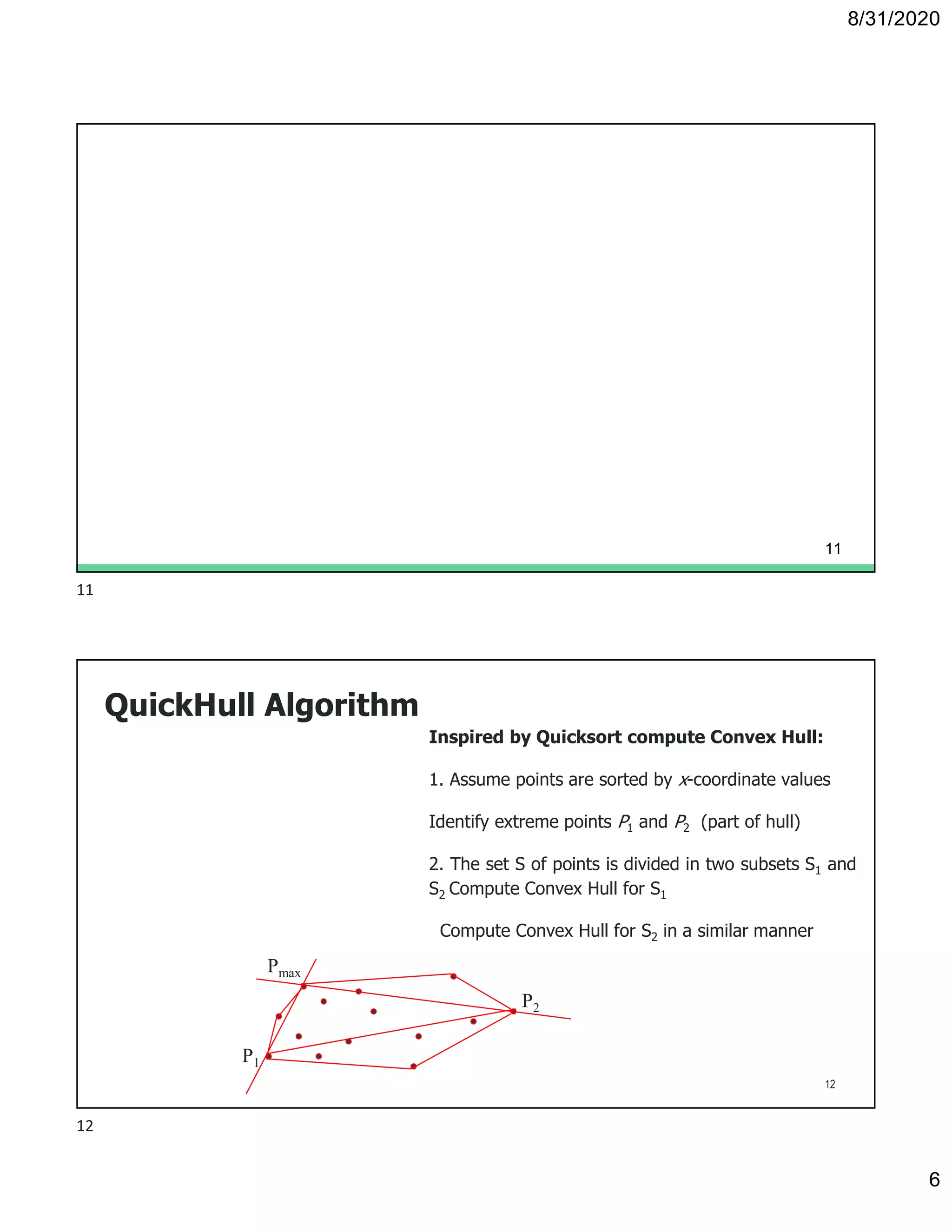
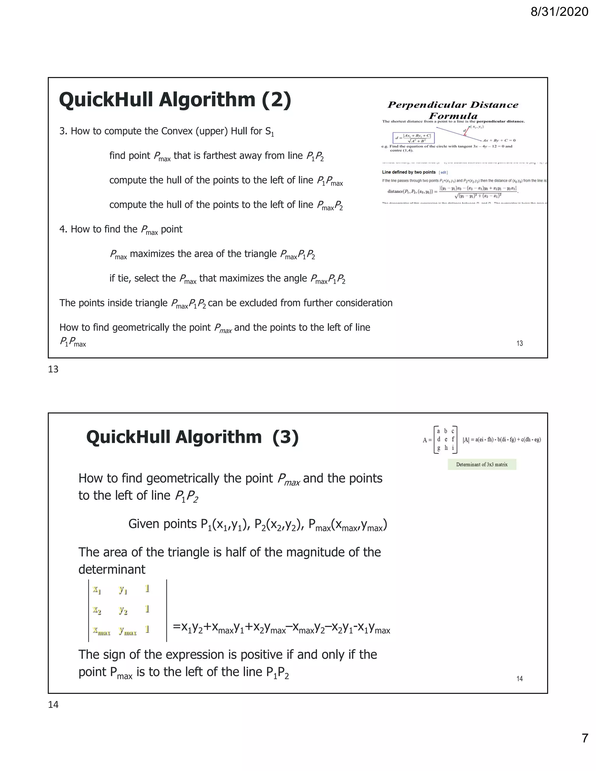
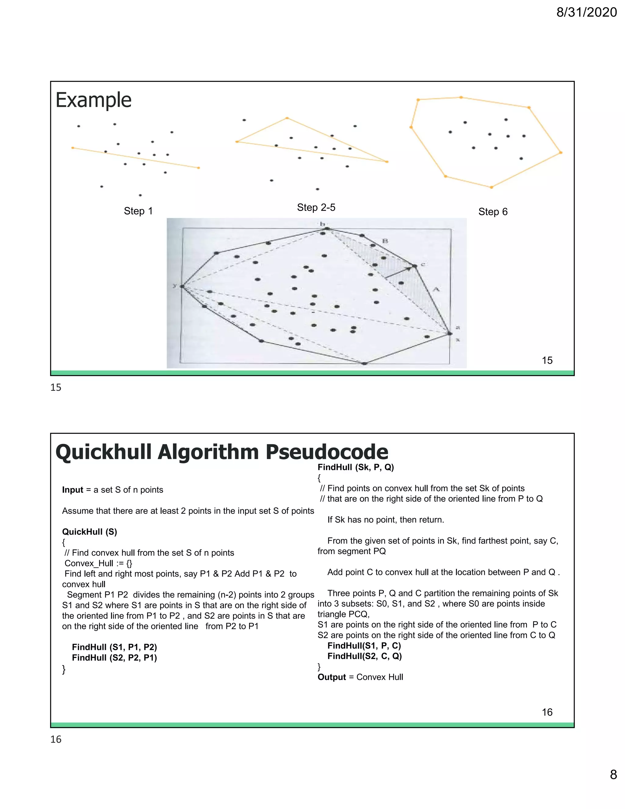
The document discusses algorithms for computing convex hulls, including Graham's scan and quickhull algorithms. Graham's scan finds the convex hull of a set of points by maintaining a stack of candidate points and removing points that are not vertices of the convex hull. It runs in O(n log n) time. Quickhull is a divide and conquer algorithm that recursively partitions points and computes farthest points to partition the space until the convex hull is completed. Both algorithms are efficient ways to compute convex hulls in two dimensions.


![8/31/2020
14
0
1
2
4
5
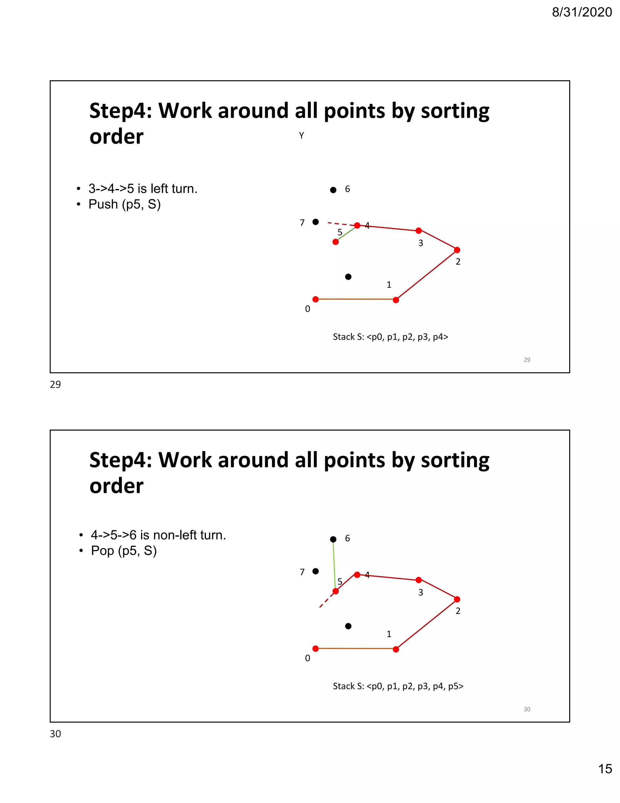
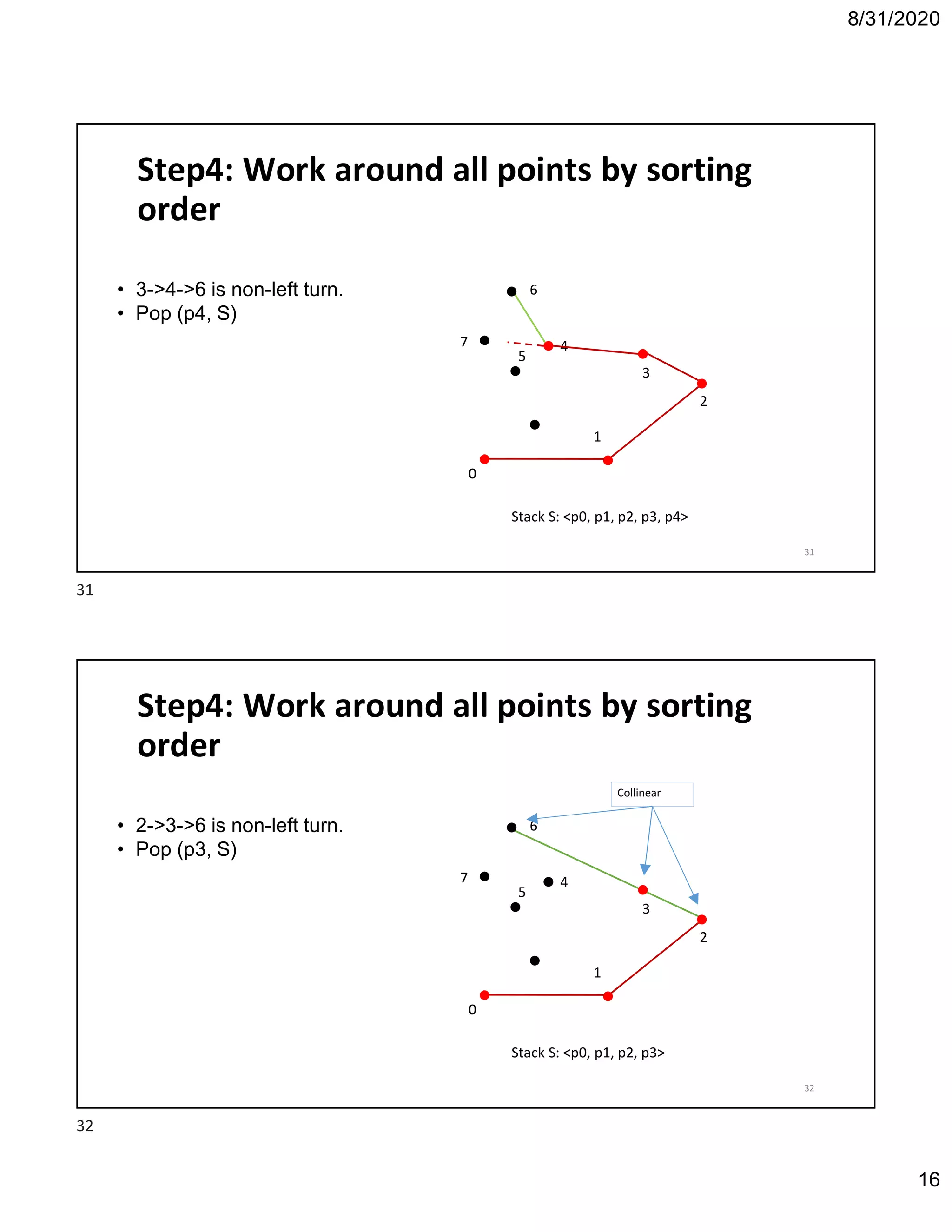
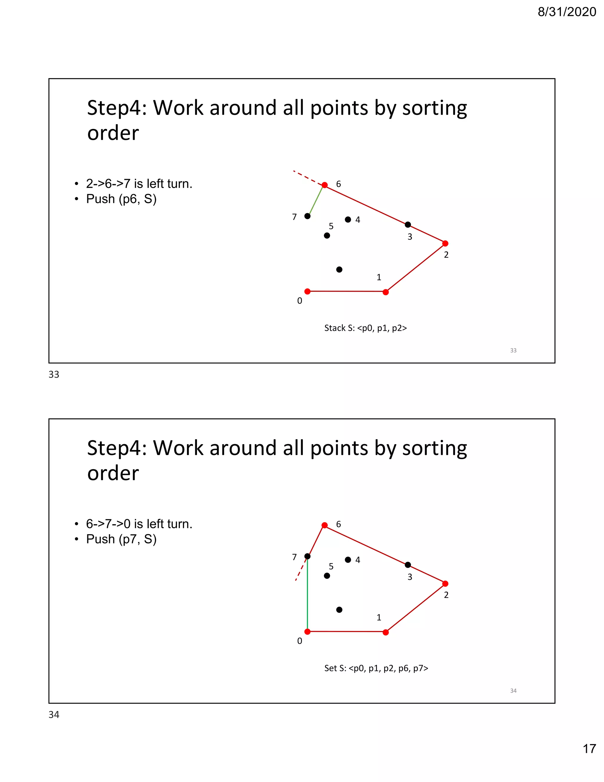
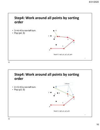
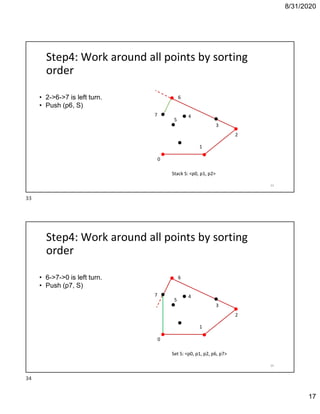
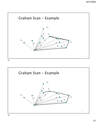
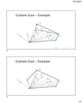
Step4: Work around all points by sorting
order
• 1->2->3 is left turn.
• Push (p3, S)
3
6
7
Next -to -top[S]
top[S]
Stack S: <p0, p1, p2>
27
Y
0
1
2
4
5
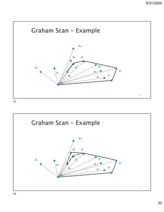
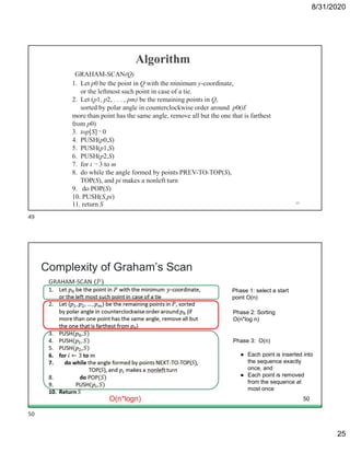
Step4: Work around all points by sorting
order
3
6• 2->3->4 is left turn.
• Push (p4, S)
7
Stack S: <p0, p1, p2, p3>
28
27
28](https://image.slidesharecdn.com/unit-iidivideandconquer-4-200831110326/85/Unit-ii-divide-and-conquer-4-14-320.jpg)


![8/31/2020
14
0
1
2
4
5
Step4: Work around all points by sorting
order
• 1->2->3 is left turn.
• Push (p3, S)
3
6
7
Next -to -top[S]
top[S]
Stack S: <p0, p1, p2>
27
Y
0
1
2
4
5
Step4: Work around all points by sorting
order
3
6• 2->3->4 is left turn.
• Push (p4, S)
7
Stack S: <p0, p1, p2, p3>
28
27
28](https://image.slidesharecdn.com/unit-iidivideandconquer-4-200831110326/75/Unit-ii-divide-and-conquer-4-14-2048.jpg)