Downloaded 516 times

![Counting sort
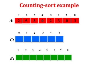
Counting sort assumes that each of the n input elements is an
integer in the range 0 to k. that is n is the number of elements and
k is the highest value element.
Consider the input set : 4, 1, 3, 4, 3. Then n=5 and k=4
Counting sort determines for each input element x, the number of
elements less than x. And it uses this information to place
element x directly into its position in the output array. For
example if there exits 17 elements less that x then x is placed into
the 18th position into the output array.
The algorithm uses three array:
Input Array: A[1..n] store input data where A[j] {1, 2, 3, …, k}
Output Array: B[1..n] finally store the sorted data
Temporary Array: C[1..k] store data temporarily](https://image.slidesharecdn.com/countingsort-140209084607-phpapp02/85/Counting-sort-Non-Comparison-Sort-10-320.jpg)
![Counting Sort
1. Counting-Sort(A, B, k)
2. Let C[0…..k] be a new array
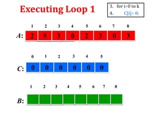
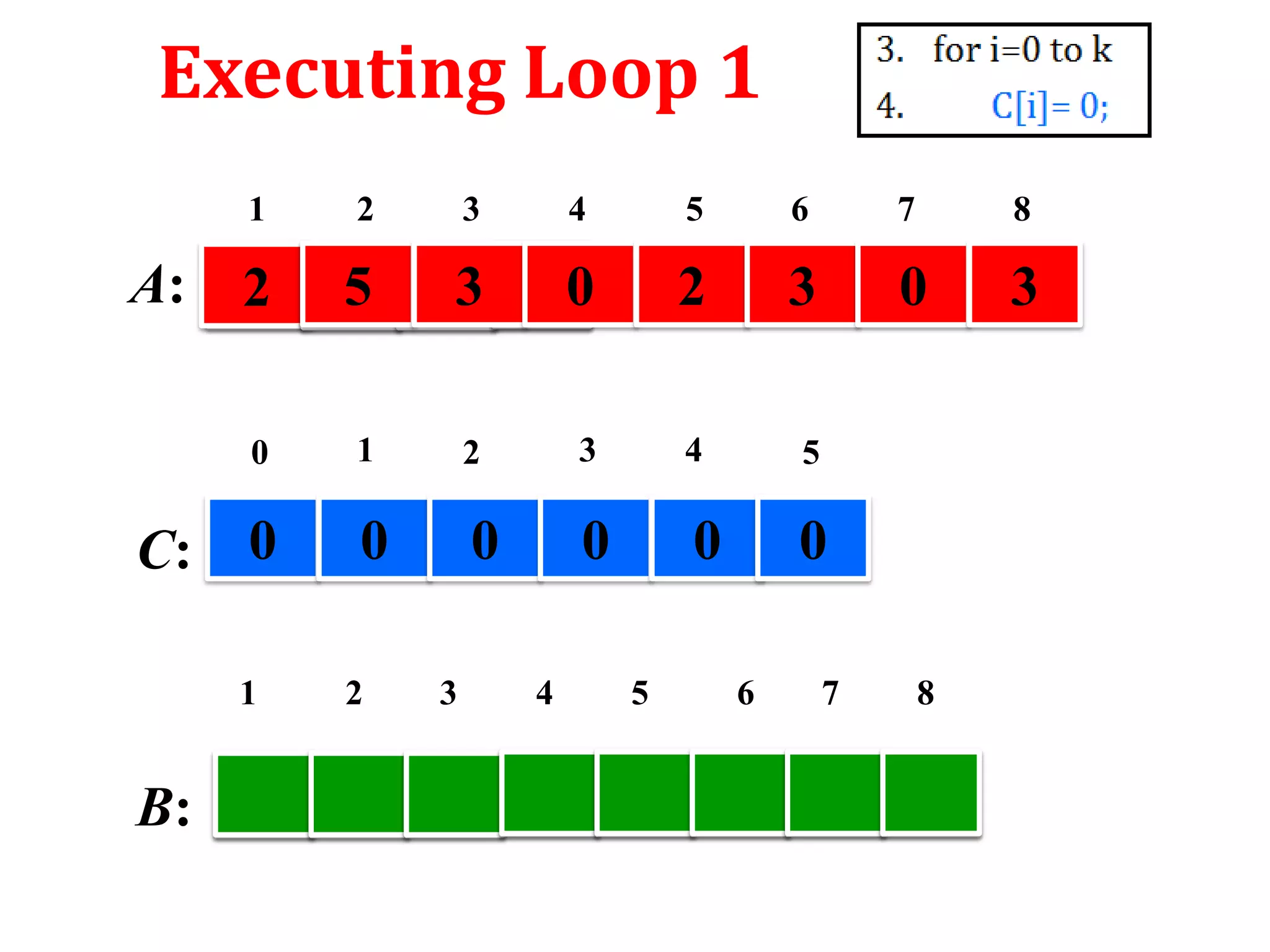
3. for i=0 to k
4.
C[i]= 0;
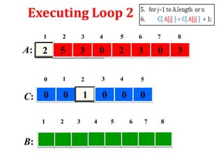
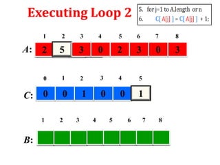
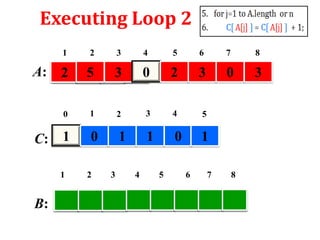
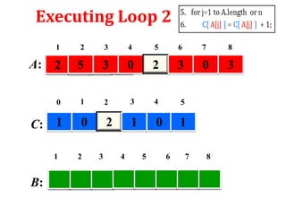
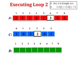
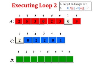
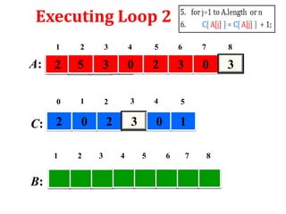
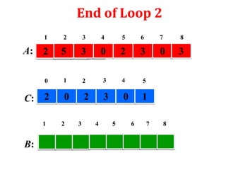
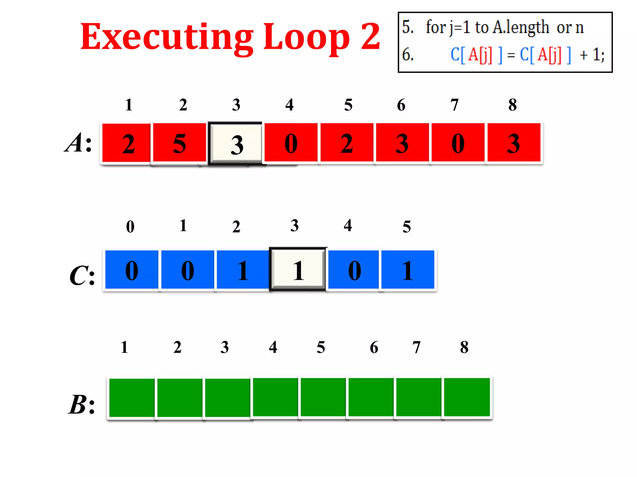
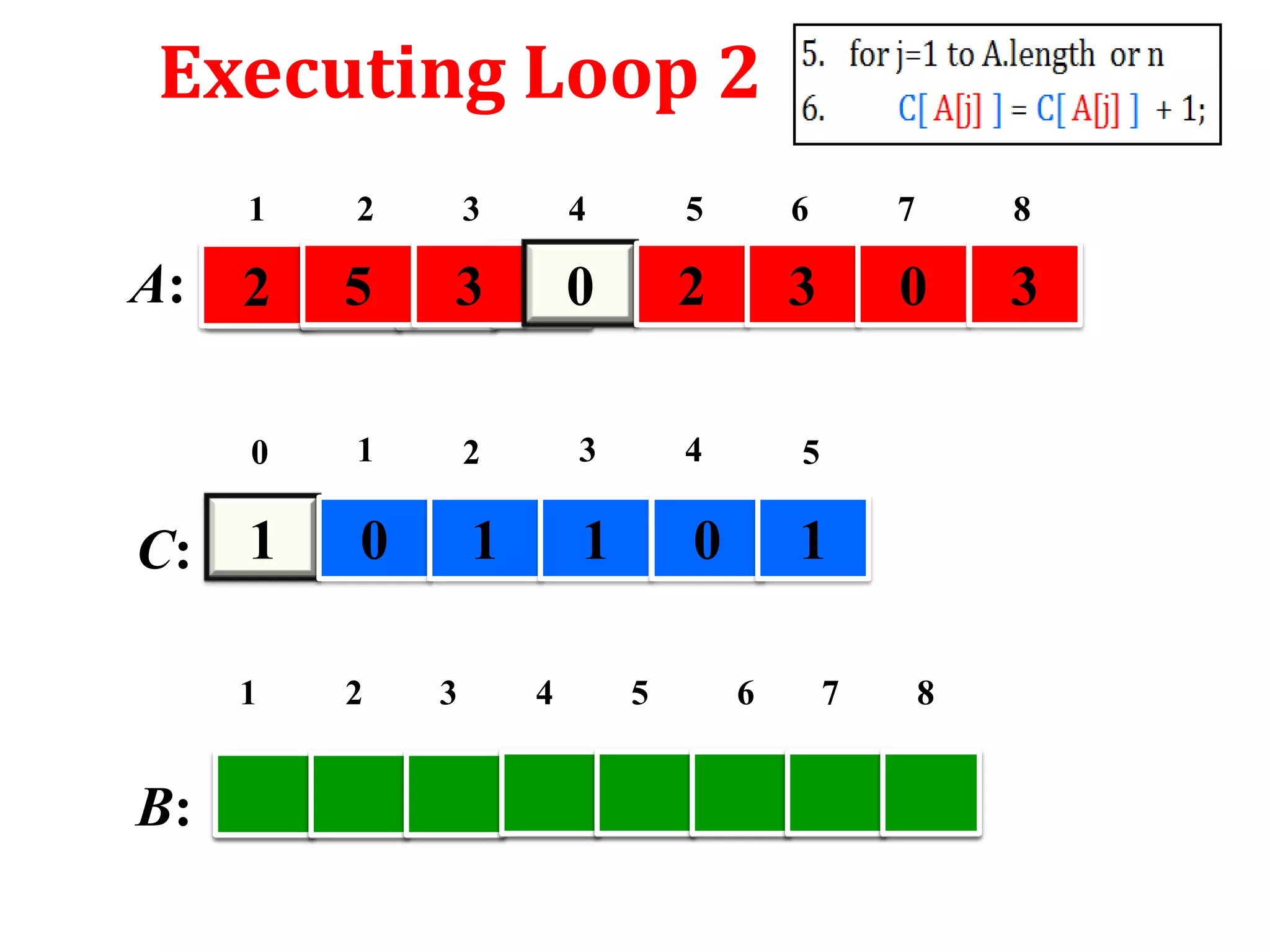
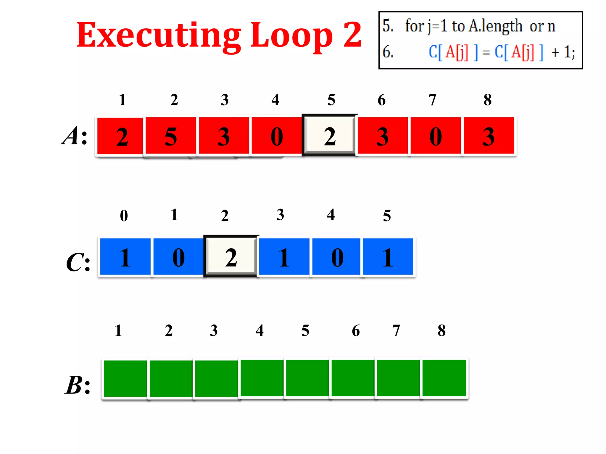
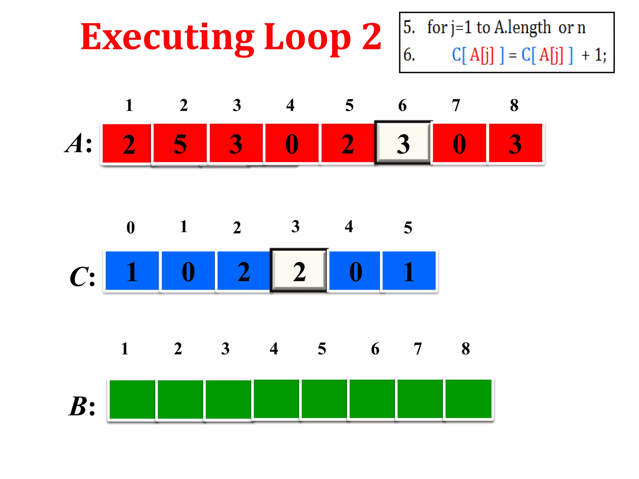
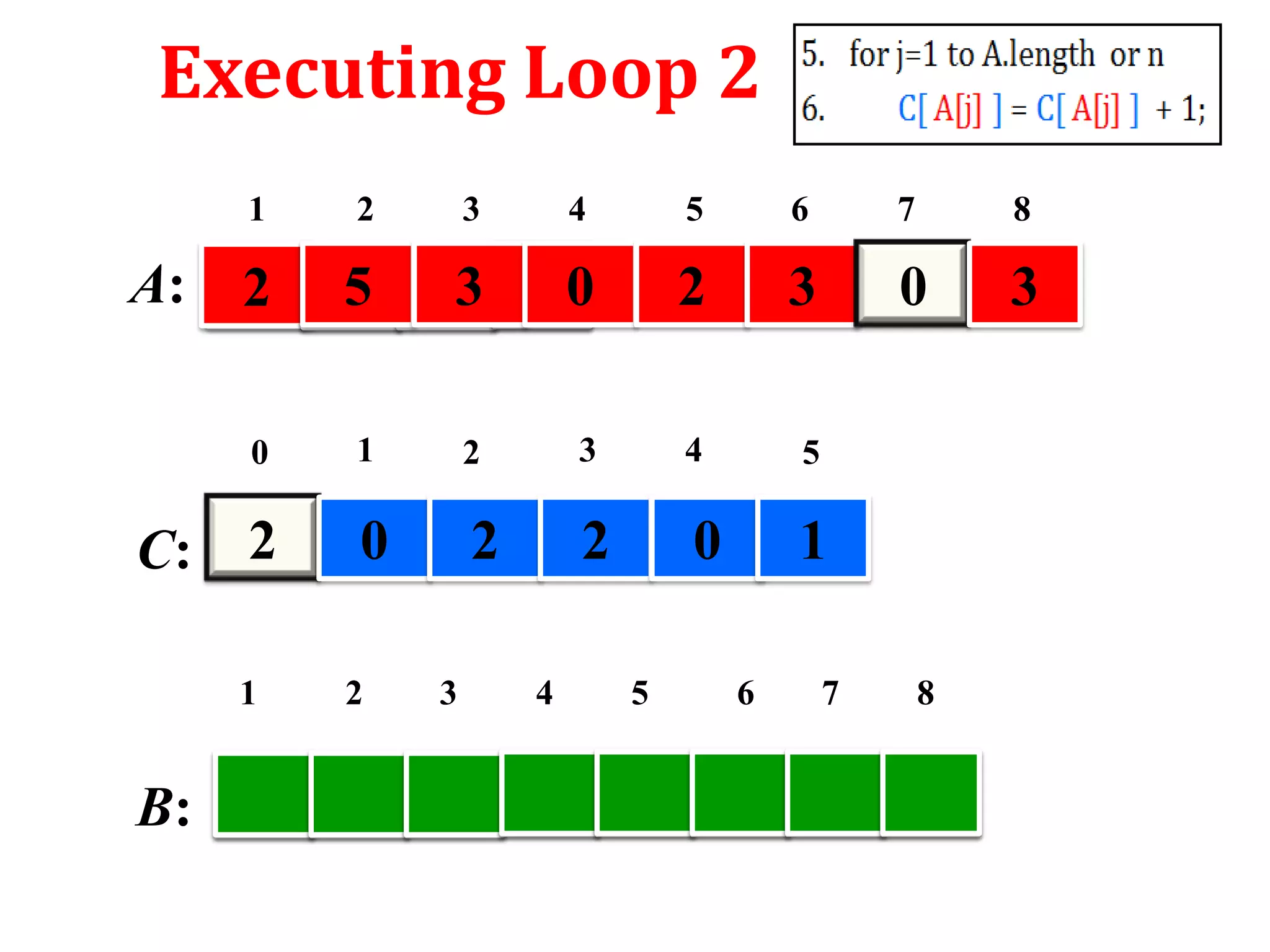
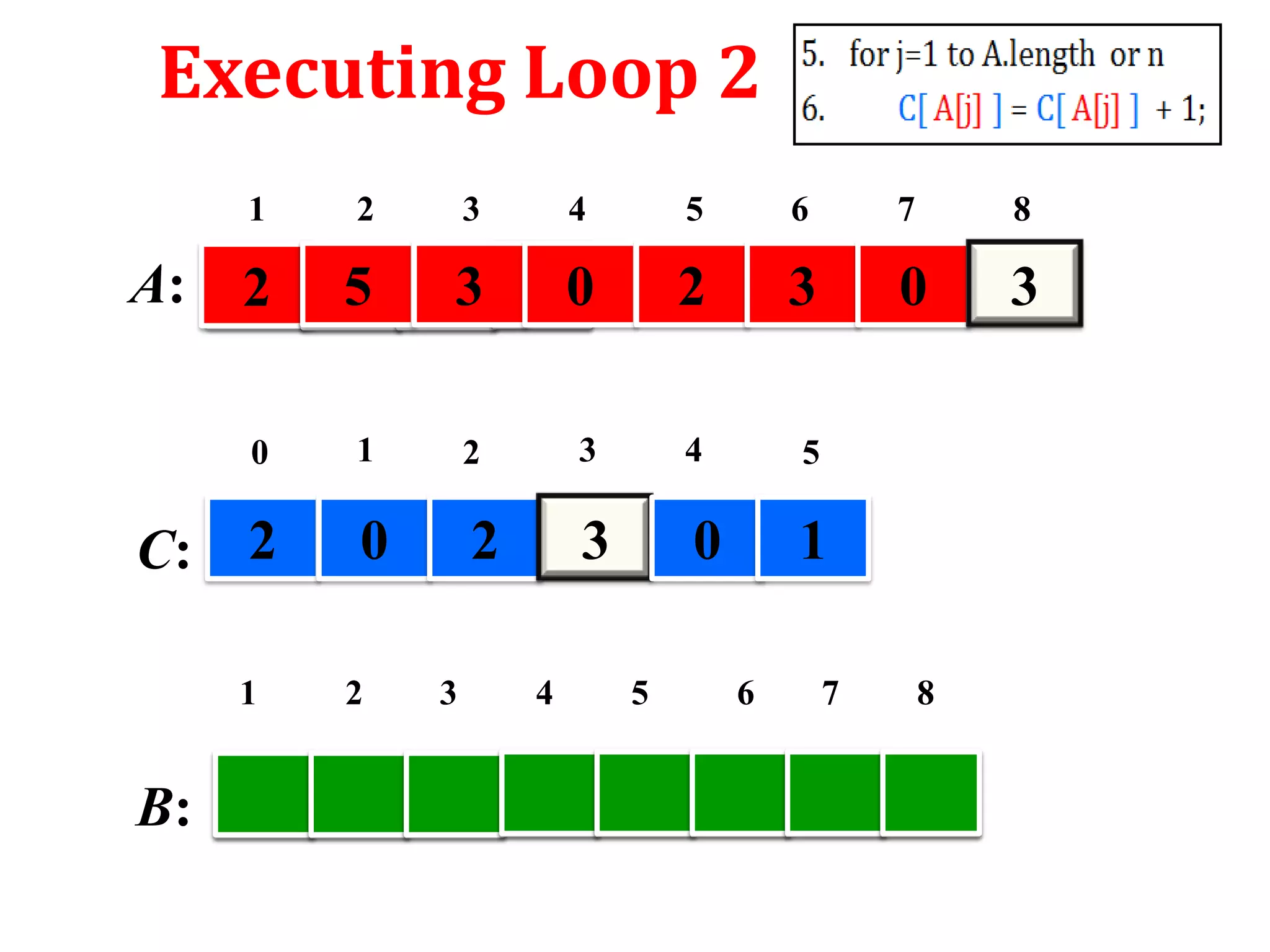
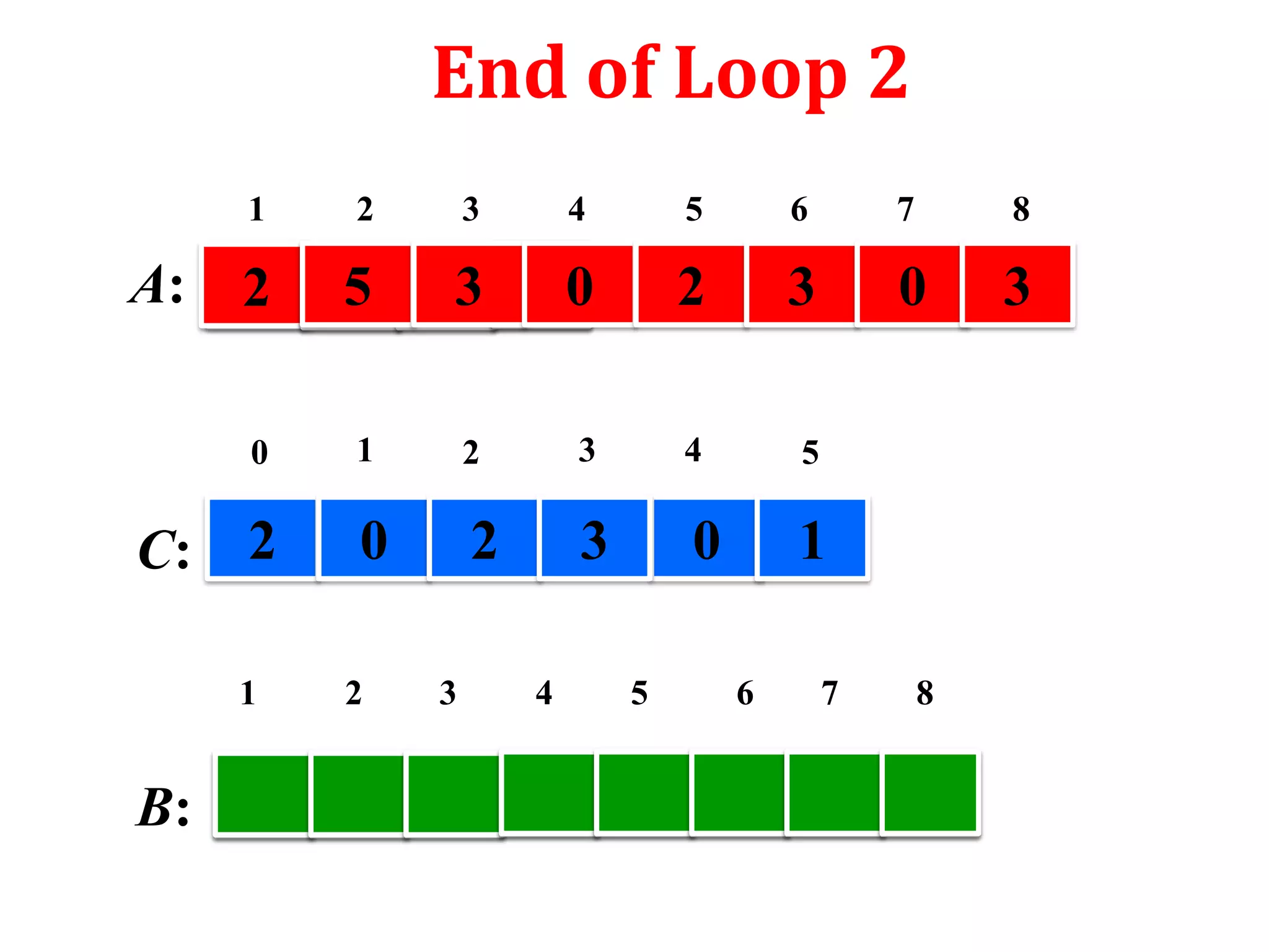
5. for j=1 to A.length or n
6.
C[ A[j] ] = C[ A[j] ] + 1;
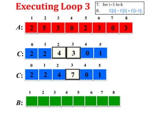
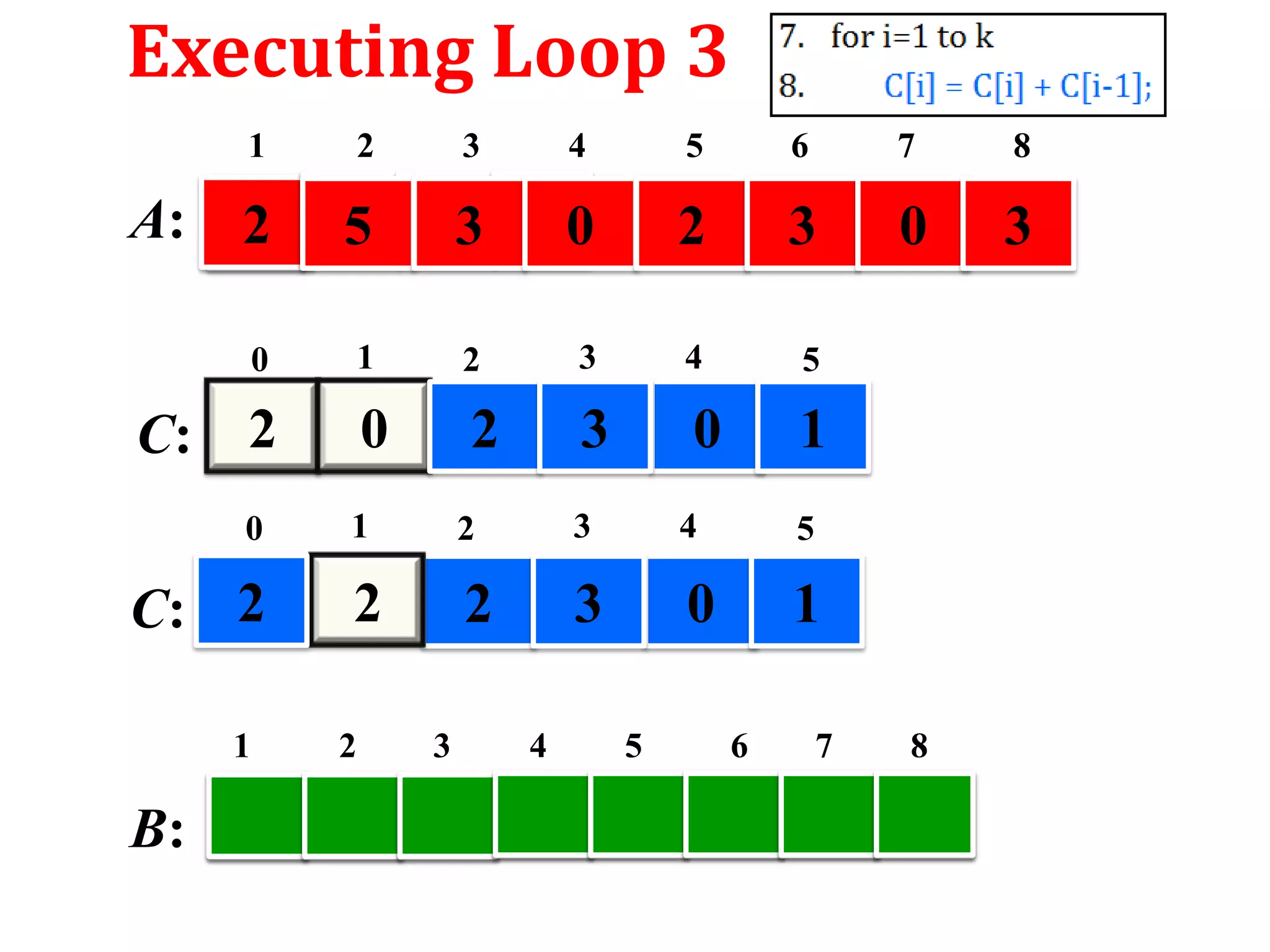
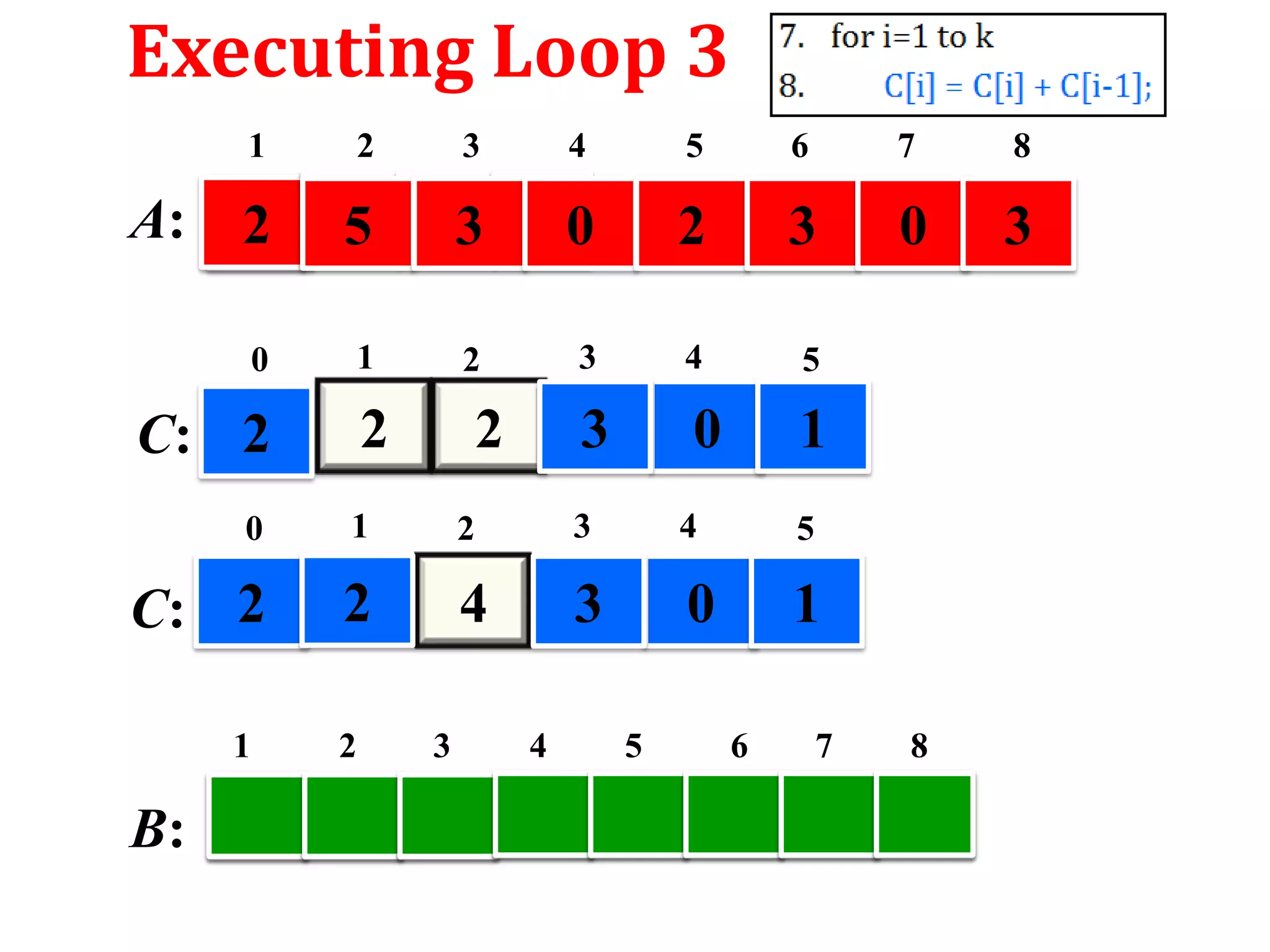
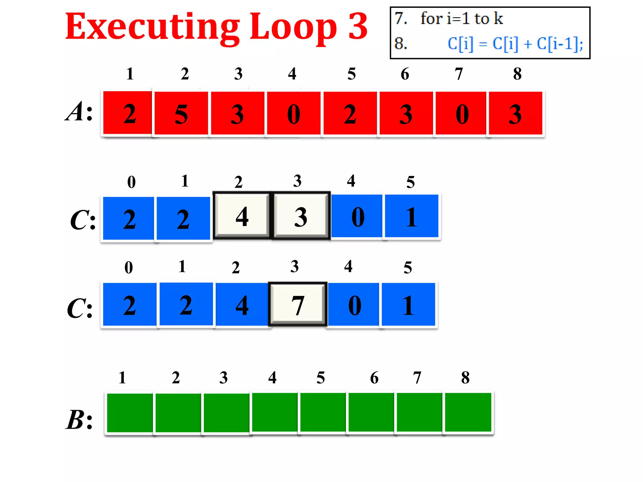
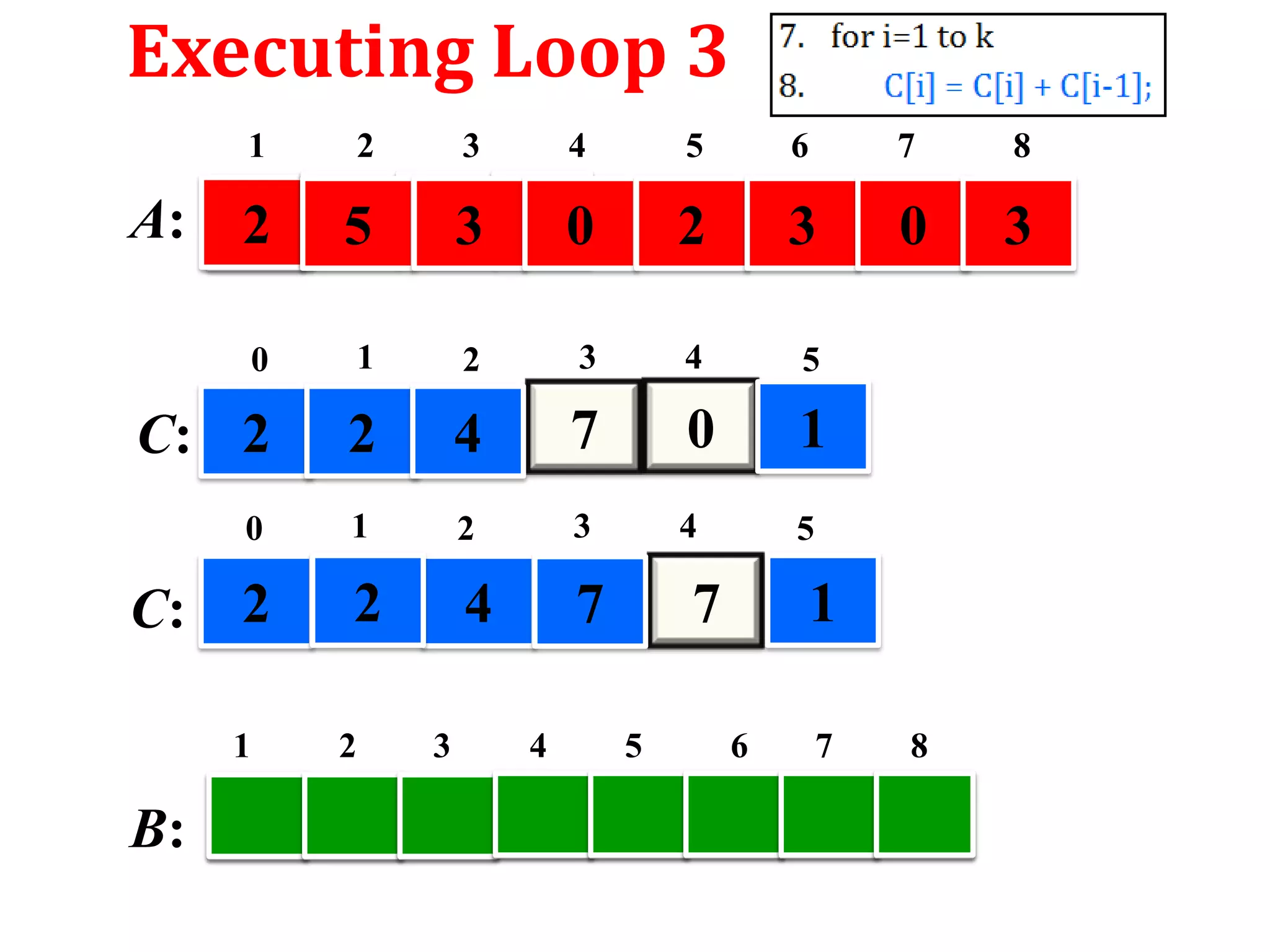
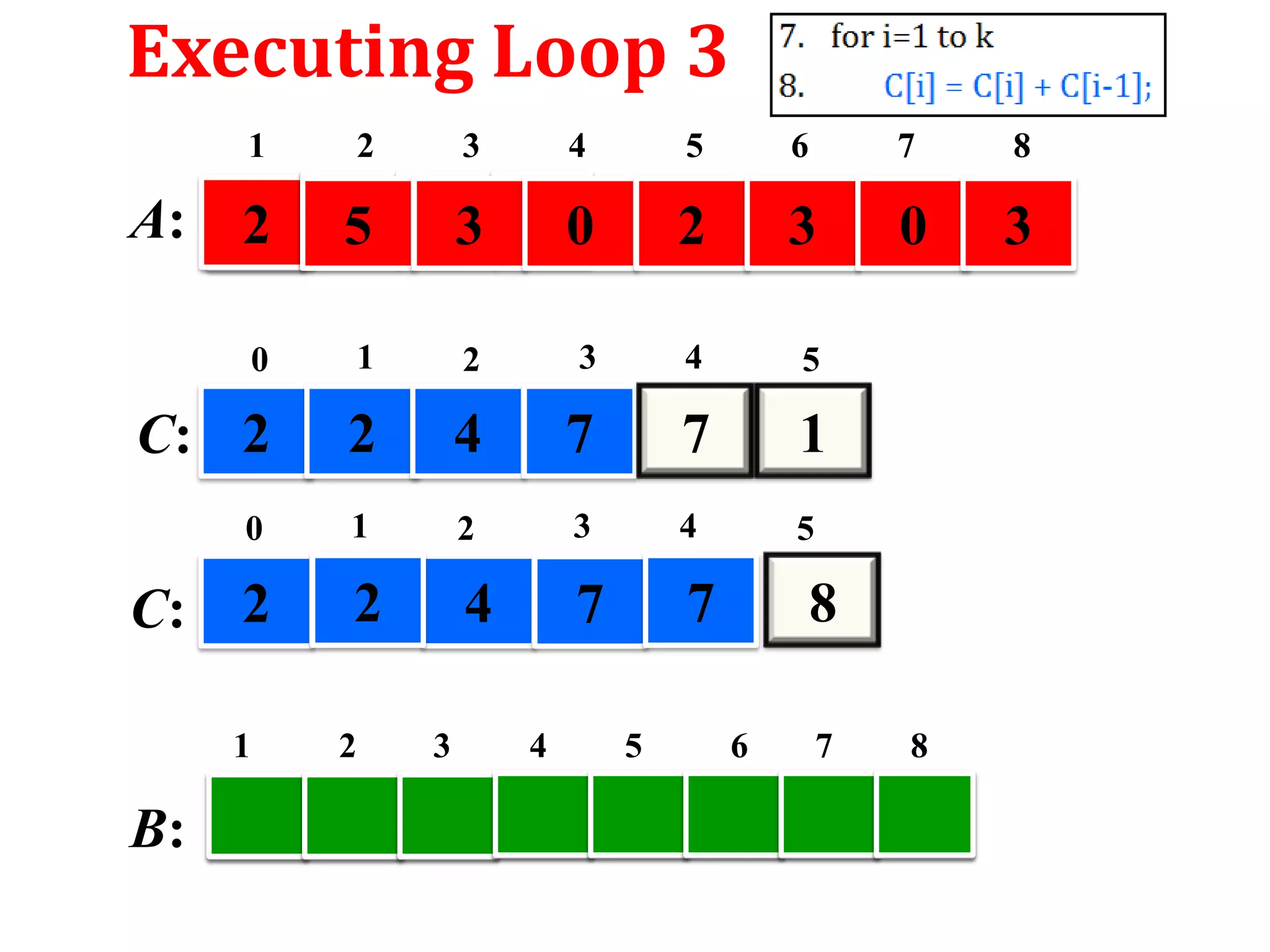
7. for i=1 to k
8.
C[i] = C[i] + C[i-1];
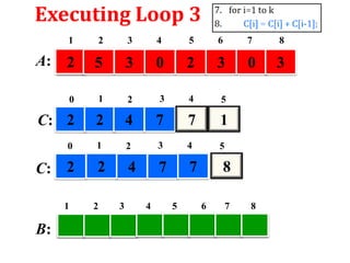
9. for j=n or A.length down to 1
10.
B[ C[ A[j] ] ] = A[j];
11.
C[ A[j] ] = C[ A[j] ] - 1;](https://image.slidesharecdn.com/countingsort-140209084607-phpapp02/85/Counting-sort-Non-Comparison-Sort-11-320.jpg)
![Counting Sort
1. Counting-Sort(A, B, k)
2. Let C[0…..k] be a new array
3. for i=0 to k
4.
C[i]= 0;
5. for j=1 to A.length or n
6.
C[ A[j] ] = C[ A[j] ] + 1;
7. for i=1 to k
8.
C[i] = C[i] + C[i-1];
9. for j=n or A.length down to 1
10.
B[ C[ A[j] ] ] = A[j];
11.
C[ A[j] ] = C[ A[j] ] - 1;
[Loop 1]
[Loop 2]
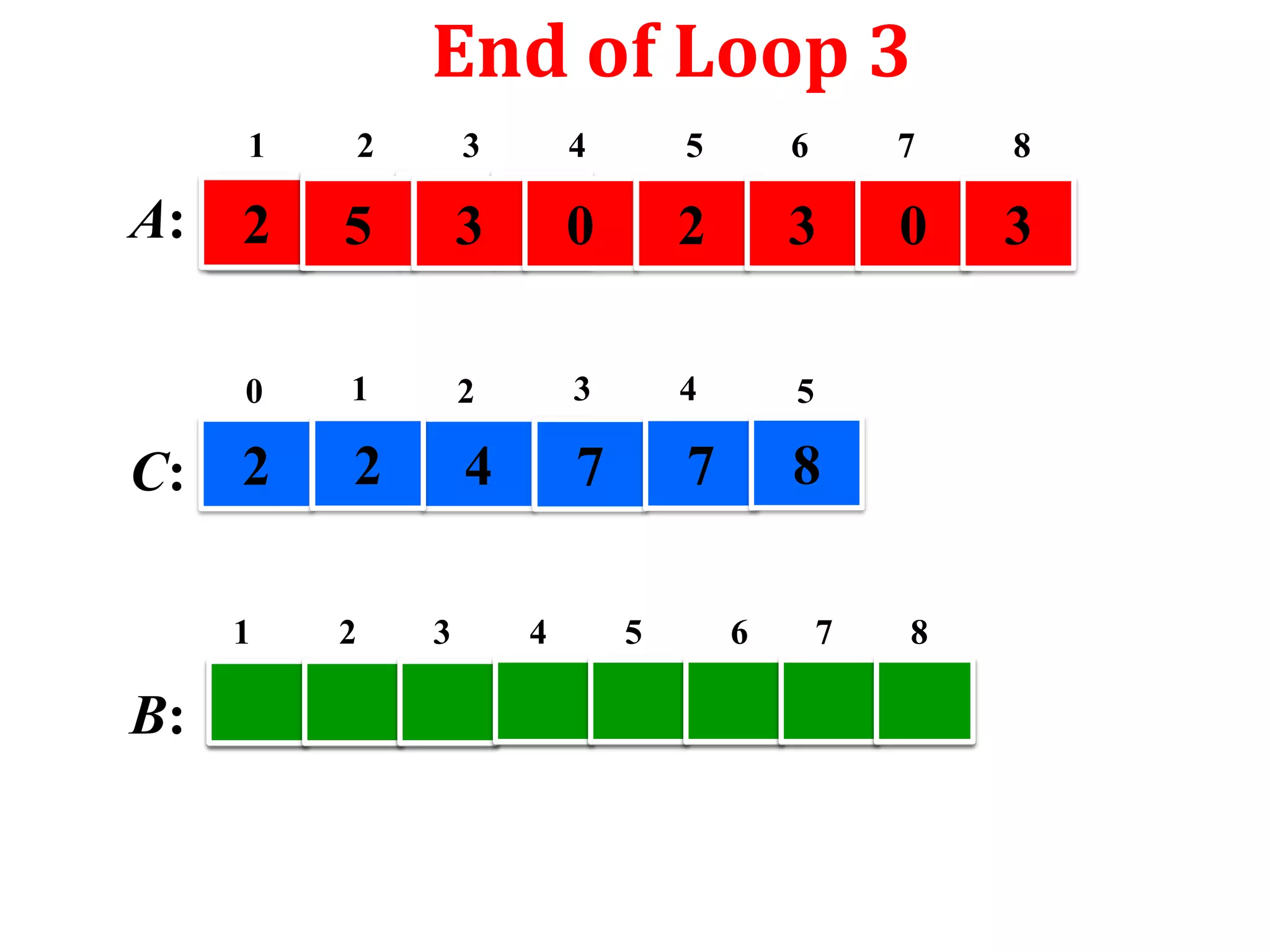
[Loop 3]
[Loop 4]](https://image.slidesharecdn.com/countingsort-140209084607-phpapp02/85/Counting-sort-Non-Comparison-Sort-12-320.jpg)


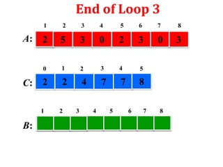
![Executing Loop 4
1
A:
2
3
4
5
6
7
8
2
5
3
0
2
3
0
3
0
C: 2
1
B:
1
2
3
4
5
2
4
7
7
8
2
3
4
5
6
7
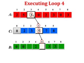
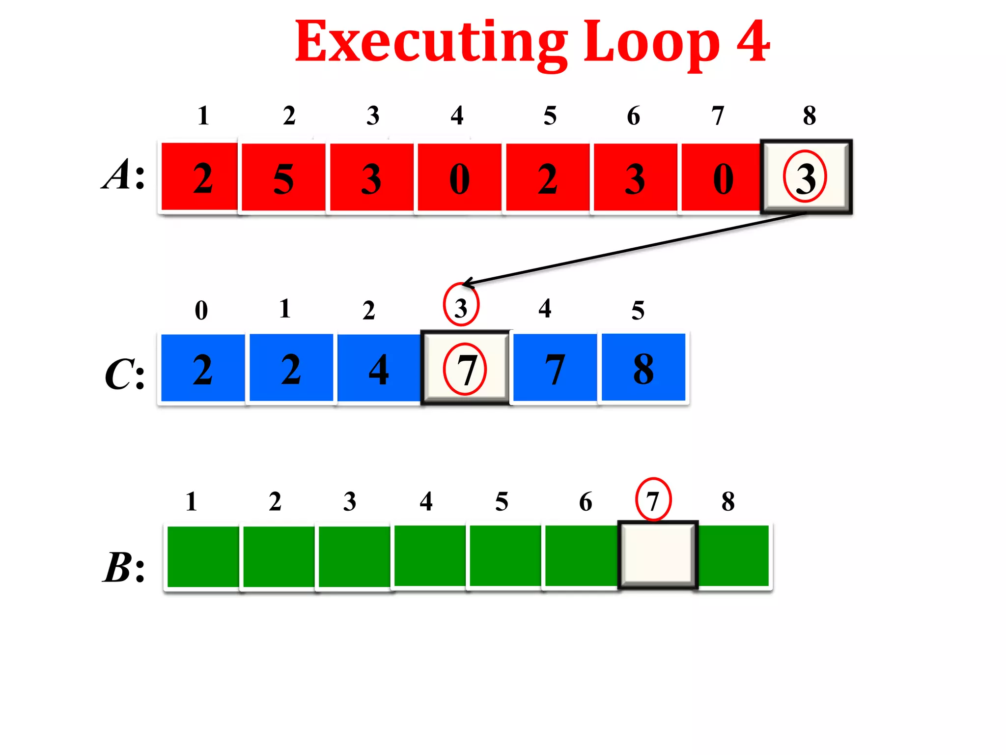
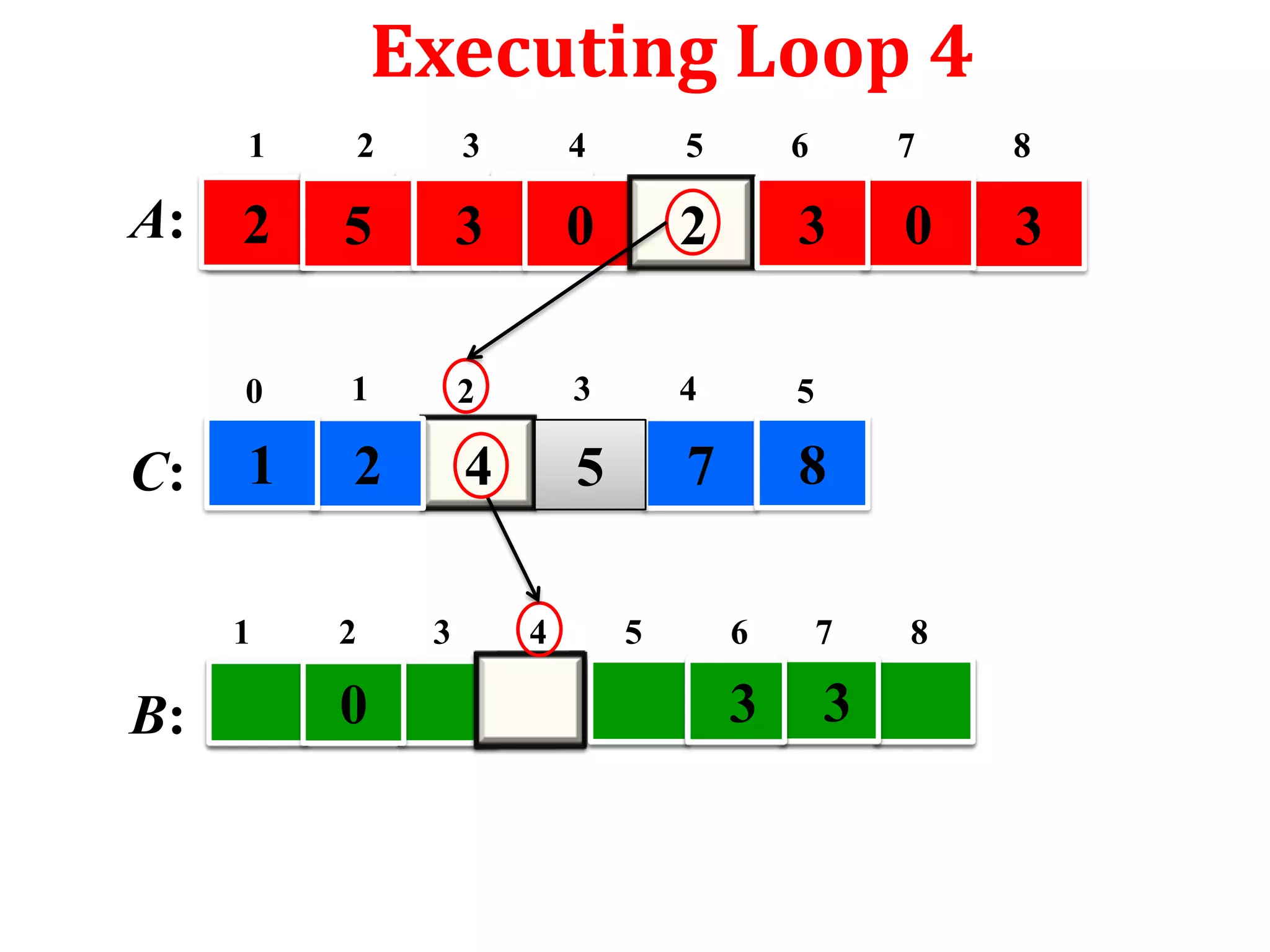
J=8, then A[ j ]=A[8]=3
And B[ C[ A[j] ] ]
=B[ C[ 3 ] ]
=B[ 7]
So B[ C[ A[j] ] ] ←A[ j ]
=B[7]←3
8](https://image.slidesharecdn.com/countingsort-140209084607-phpapp02/85/Counting-sort-Non-Comparison-Sort-31-320.jpg)
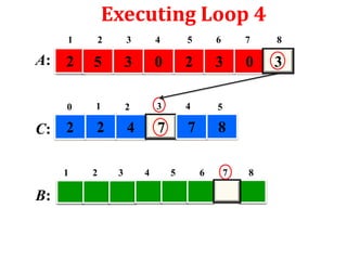
![Executing Loop 4
1
A:
2
3
4
5
6
7
8
2
5
3
0
2
3
0
3
0
C:
1
2
3
4
5
2
2
4
6
7
8
1
B:
2
3
4
5
6
7
3
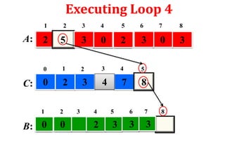
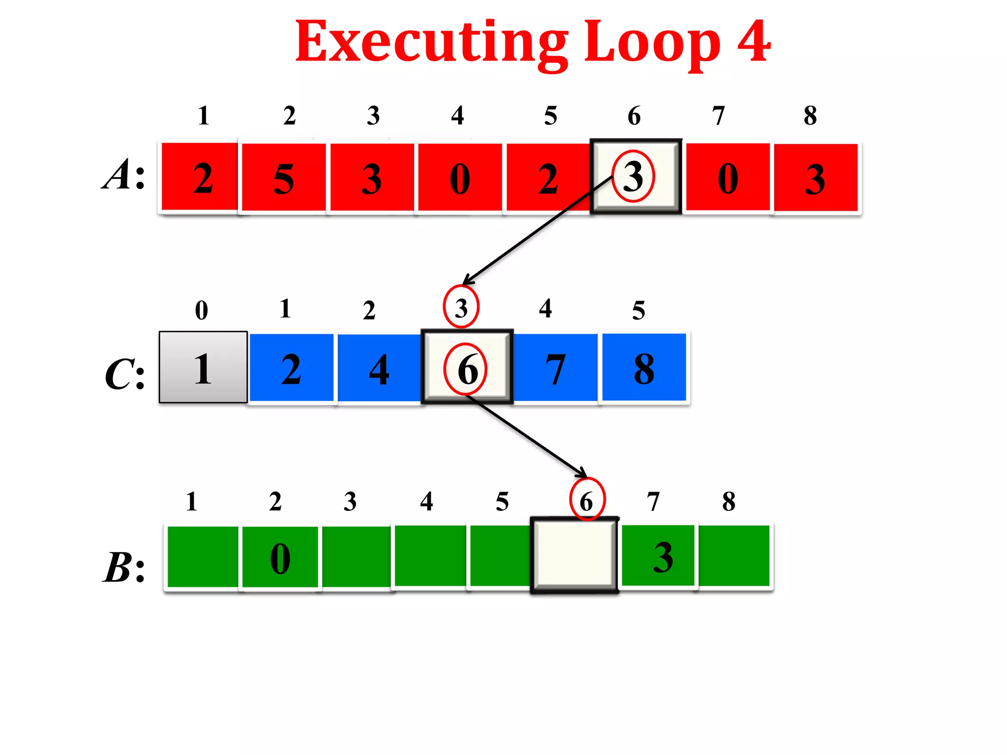
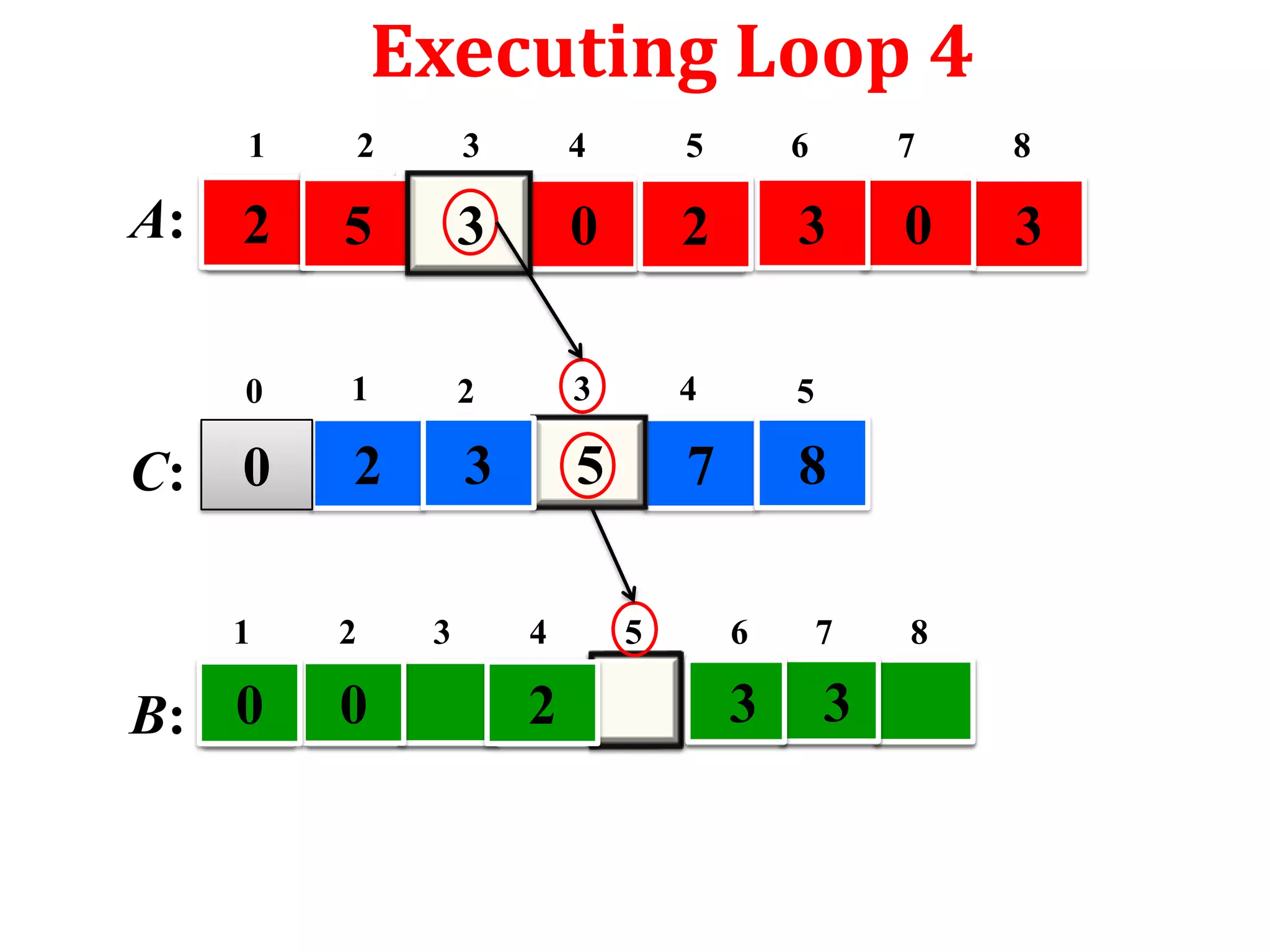
J=8, then A[ j ]=A[8]=3
Then C[ A[j] ]
= C[ 3 ]
=7
So C[ A[j] ] = C[ A[j] ] -1
=7-1=6
8](https://image.slidesharecdn.com/countingsort-140209084607-phpapp02/85/Counting-sort-Non-Comparison-Sort-32-320.jpg)


![Time Complexity Analysis
1. Counting-Sort(A, B, k)
2. Let C[0…..k] be a new array
3. for i=0 to k
4.
C[i]= 0;
5. for j=1 to A.length or n
6.
C[ A[j] ] = C[ A[j] ] + 1;
7. for i=1 to k
8.
C[i] = C[i] + C[i-1];
9. for j=n or A.length down to 1
10.
B[ C[ A[j] ] ] = A[j];
11.
C[ A[j] ] = C[ A[j] ] - 1;
[Loop 1]
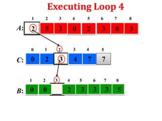
Loop 1 and 3
takes O(k) time
[Loop 2]
[Loop 3]
[Loop 4]
Loop 2 and 4
takes O(n) time](https://image.slidesharecdn.com/countingsort-140209084607-phpapp02/85/Counting-sort-Non-Comparison-Sort-40-320.jpg)


![Counting sort
Counting sort assumes that each of the n input elements is an
integer in the range 0 to k. that is n is the number of elements and
k is the highest value element.
Consider the input set : 4, 1, 3, 4, 3. Then n=5 and k=4
Counting sort determines for each input element x, the number of
elements less than x. And it uses this information to place
element x directly into its position in the output array. For
example if there exits 17 elements less that x then x is placed into
the 18th position into the output array.
The algorithm uses three array:
Input Array: A[1..n] store input data where A[j] {1, 2, 3, …, k}
Output Array: B[1..n] finally store the sorted data
Temporary Array: C[1..k] store data temporarily](https://image.slidesharecdn.com/countingsort-140209084607-phpapp02/75/Counting-sort-Non-Comparison-Sort-10-2048.jpg)
![Counting Sort
1. Counting-Sort(A, B, k)
2. Let C[0…..k] be a new array
3. for i=0 to k
4.
C[i]= 0;
5. for j=1 to A.length or n
6.
C[ A[j] ] = C[ A[j] ] + 1;
7. for i=1 to k
8.
C[i] = C[i] + C[i-1];
9. for j=n or A.length down to 1
10.
B[ C[ A[j] ] ] = A[j];
11.
C[ A[j] ] = C[ A[j] ] - 1;](https://image.slidesharecdn.com/countingsort-140209084607-phpapp02/75/Counting-sort-Non-Comparison-Sort-11-2048.jpg)
![Counting Sort
1. Counting-Sort(A, B, k)
2. Let C[0…..k] be a new array
3. for i=0 to k
4.
C[i]= 0;
5. for j=1 to A.length or n
6.
C[ A[j] ] = C[ A[j] ] + 1;
7. for i=1 to k
8.
C[i] = C[i] + C[i-1];
9. for j=n or A.length down to 1
10.
B[ C[ A[j] ] ] = A[j];
11.
C[ A[j] ] = C[ A[j] ] - 1;
[Loop 1]
[Loop 2]
[Loop 3]
[Loop 4]](https://image.slidesharecdn.com/countingsort-140209084607-phpapp02/75/Counting-sort-Non-Comparison-Sort-12-2048.jpg)


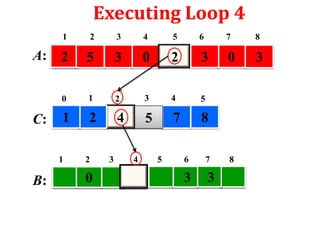
![Executing Loop 4
1
A:
2
3
4
5
6
7
8
2
5
3
0
2
3
0
3
0
C: 2
1
B:
1
2
3
4
5
2
4
7
7
8
2
3
4
5
6
7
J=8, then A[ j ]=A[8]=3
And B[ C[ A[j] ] ]
=B[ C[ 3 ] ]
=B[ 7]
So B[ C[ A[j] ] ] ←A[ j ]
=B[7]←3
8](https://image.slidesharecdn.com/countingsort-140209084607-phpapp02/75/Counting-sort-Non-Comparison-Sort-31-2048.jpg)
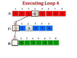
![Executing Loop 4
1
A:
2
3
4
5
6
7
8
2
5
3
0
2
3
0
3
0
C:
1
2
3
4
5
2
2
4
6
7
8
1
B:
2
3
4
5
6
7
3
J=8, then A[ j ]=A[8]=3
Then C[ A[j] ]
= C[ 3 ]
=7
So C[ A[j] ] = C[ A[j] ] -1
=7-1=6
8](https://image.slidesharecdn.com/countingsort-140209084607-phpapp02/75/Counting-sort-Non-Comparison-Sort-32-2048.jpg)

![Time Complexity Analysis
1. Counting-Sort(A, B, k)
2. Let C[0…..k] be a new array
3. for i=0 to k
4.
C[i]= 0;
5. for j=1 to A.length or n
6.
C[ A[j] ] = C[ A[j] ] + 1;
7. for i=1 to k
8.
C[i] = C[i] + C[i-1];
9. for j=n or A.length down to 1
10.
B[ C[ A[j] ] ] = A[j];
11.
C[ A[j] ] = C[ A[j] ] - 1;
[Loop 1]
Loop 1 and 3
takes O(k) time
[Loop 2]
[Loop 3]
[Loop 4]
Loop 2 and 4
takes O(n) time](https://image.slidesharecdn.com/countingsort-140209084607-phpapp02/75/Counting-sort-Non-Comparison-Sort-40-2048.jpg)


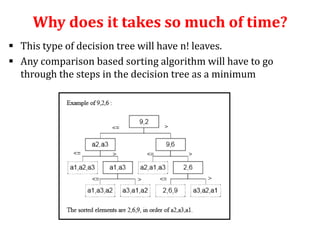
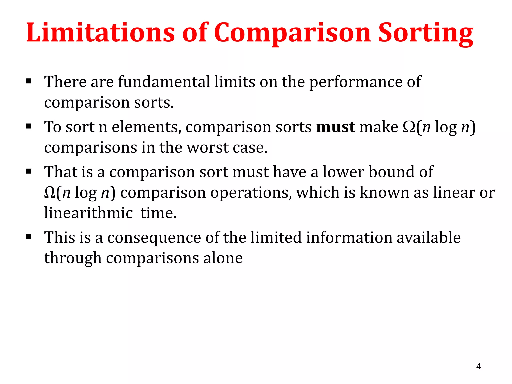
Comparison sorting algorithms work by making pairwise comparisons between elements to determine the order in a sorted list. They have a lower bound of Ω(n log n) time complexity due to needing to traverse a decision tree with a minimum of n log n comparisons. Counting sort is a non-comparison sorting algorithm that takes advantage of key assumptions about the data to count and place elements directly into the output array in linear time O(n+k), where n is the number of elements and k is the range of possible key values.
Introduces sorting algorithms and their significance in computer science.
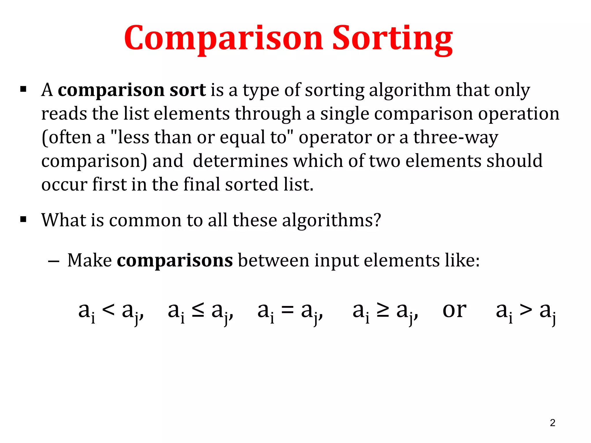
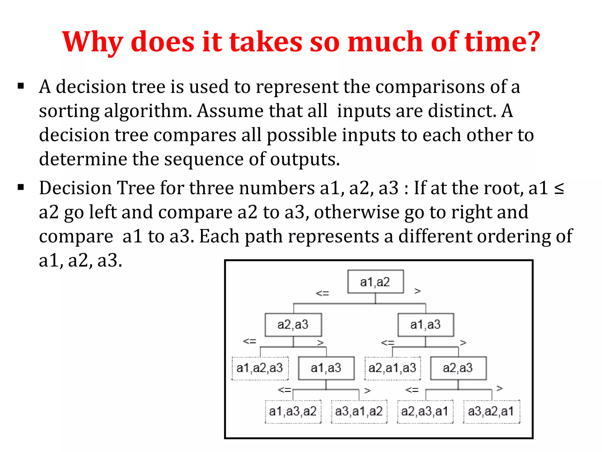
Defines comparison sorting algorithms that determine order through pairwise element comparisons.
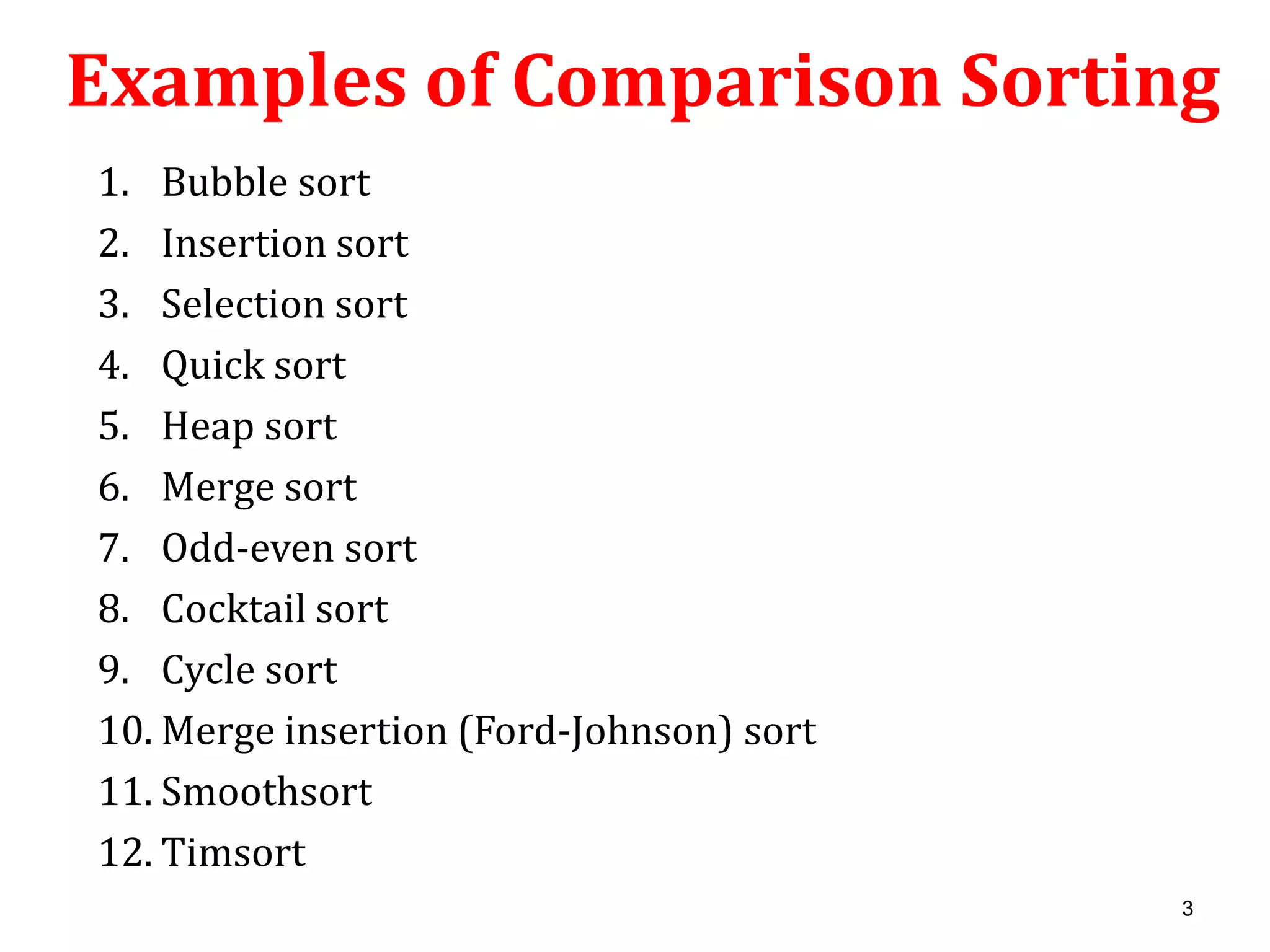
Lists examples of various comparison sorting algorithms including Bubble sort, Quick sort, and Merge sort.
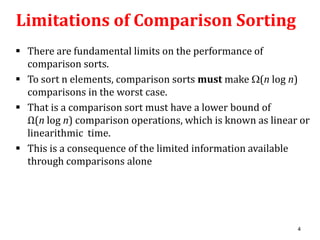
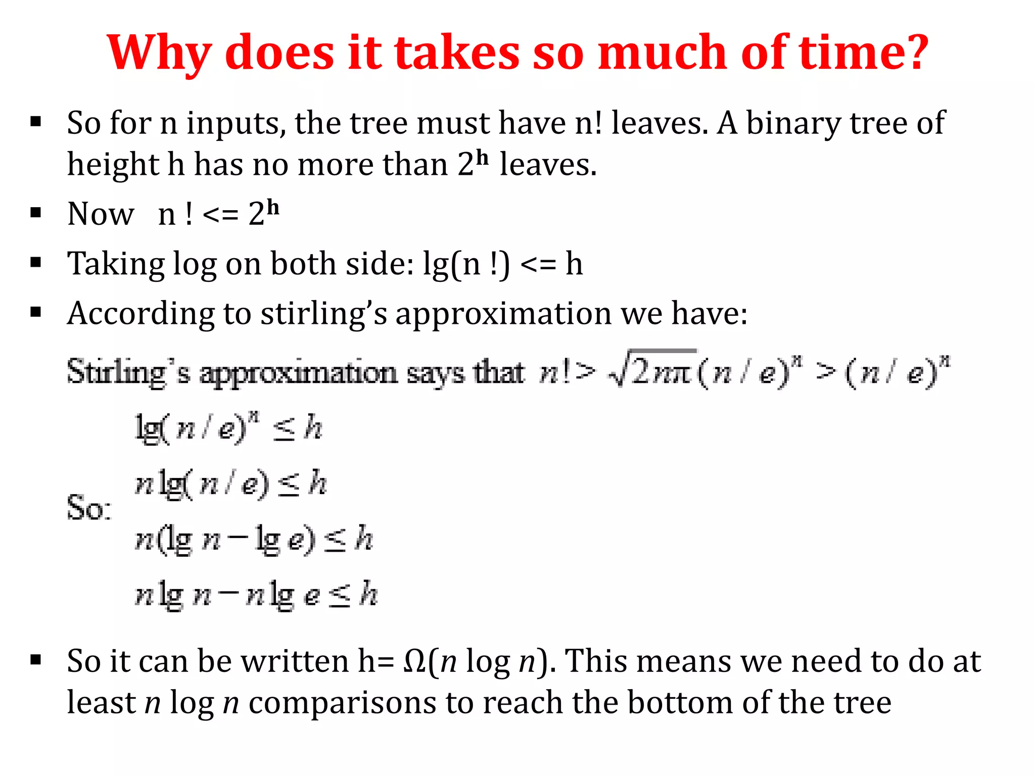
Explains the performance limitations of comparison sorts with a lower bound of Ω(n log n) comparisons.
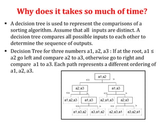
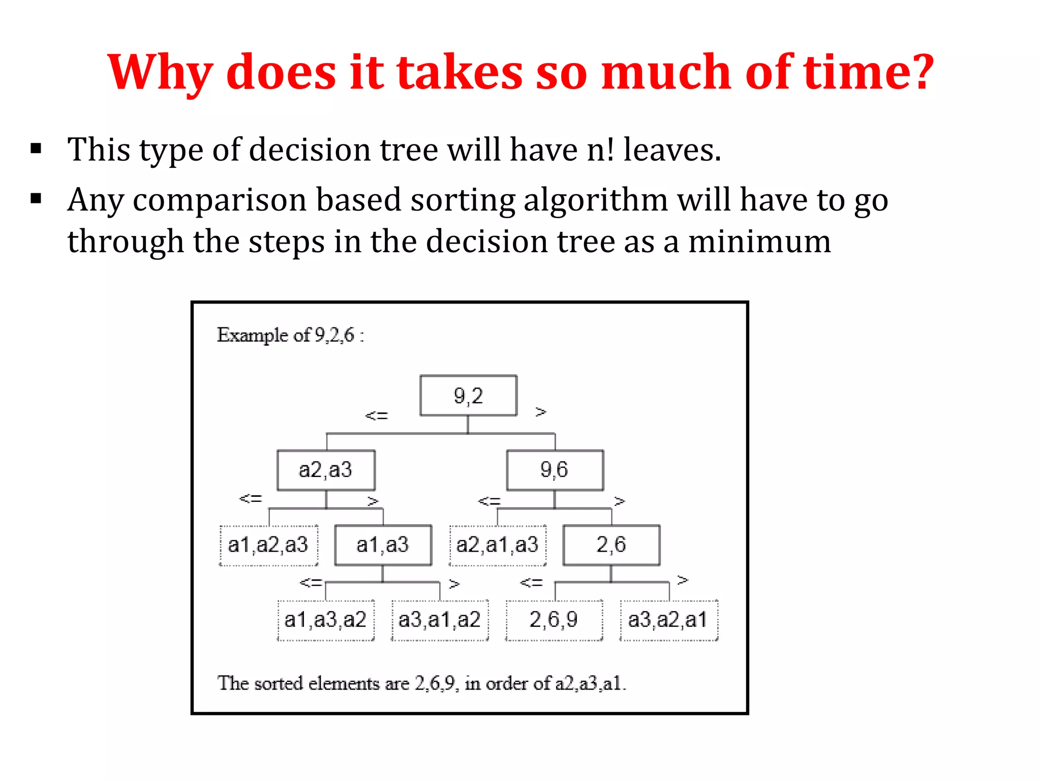
Describes decision trees used in sorting, detailing their structure and the minimum comparisons for sorting n elements.
Details the time complexity of various sorting algorithms including O(n²) and O(n log n) complexities.
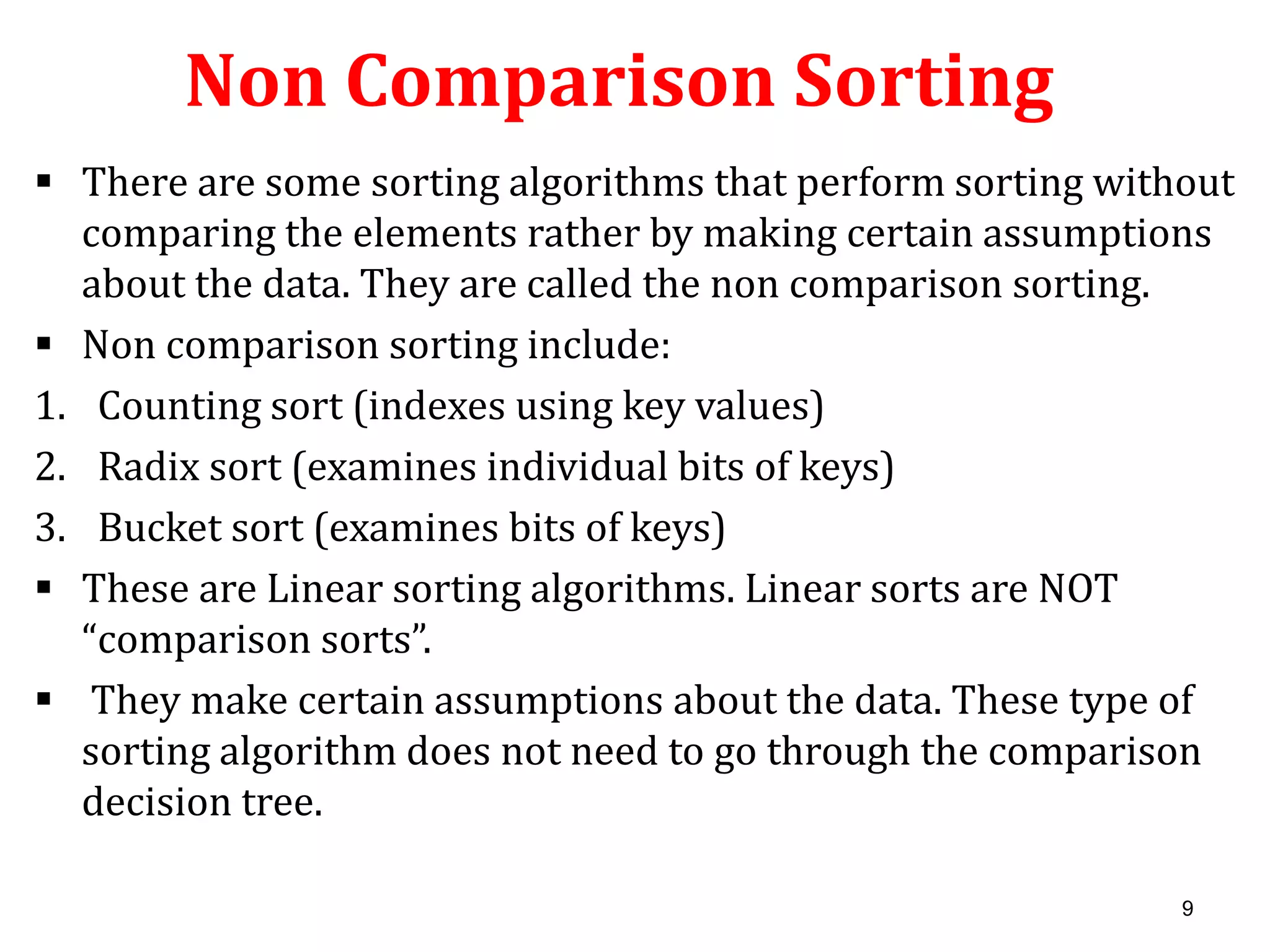
Introduces non-comparison sorting algorithms such as Counting sort, Radix sort, and Bucket sort.
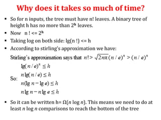
Explains the Counting Sort algorithm, its mechanism, and the arrays used in the process.
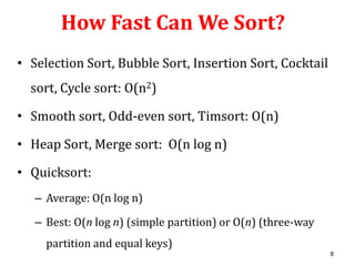
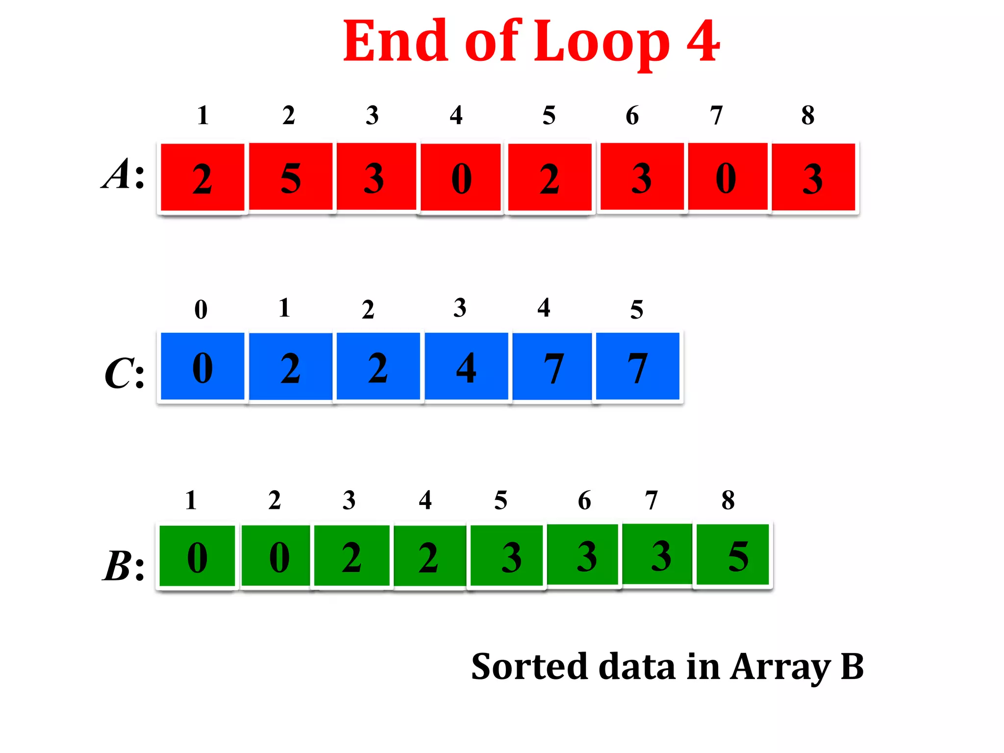
Details step-by-step execution of Counting Sort through examples and iterative loops.
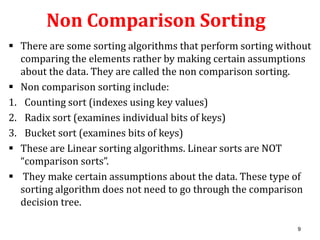
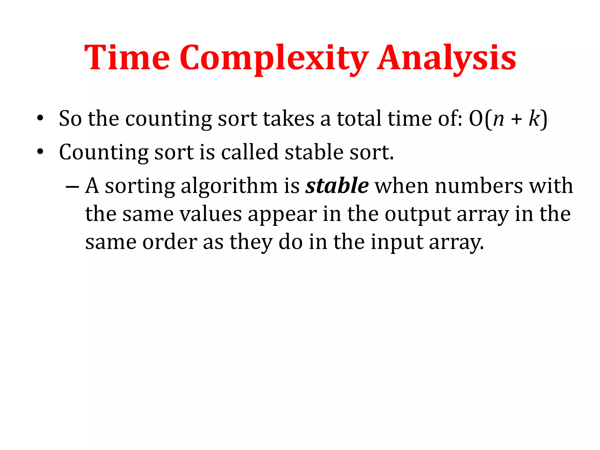
Analyzes the overall time complexity of Counting Sort, noting its efficiency and stability.
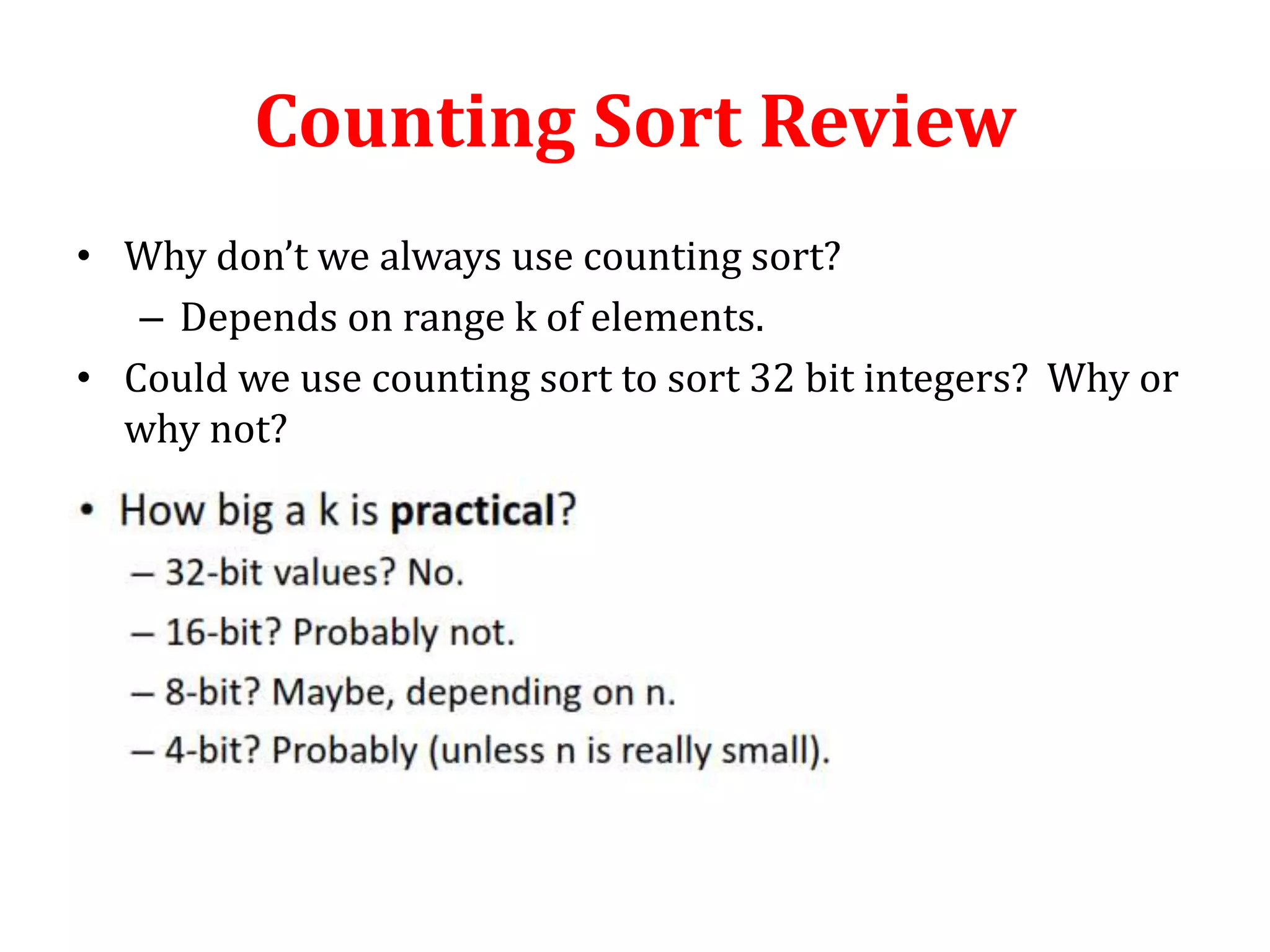
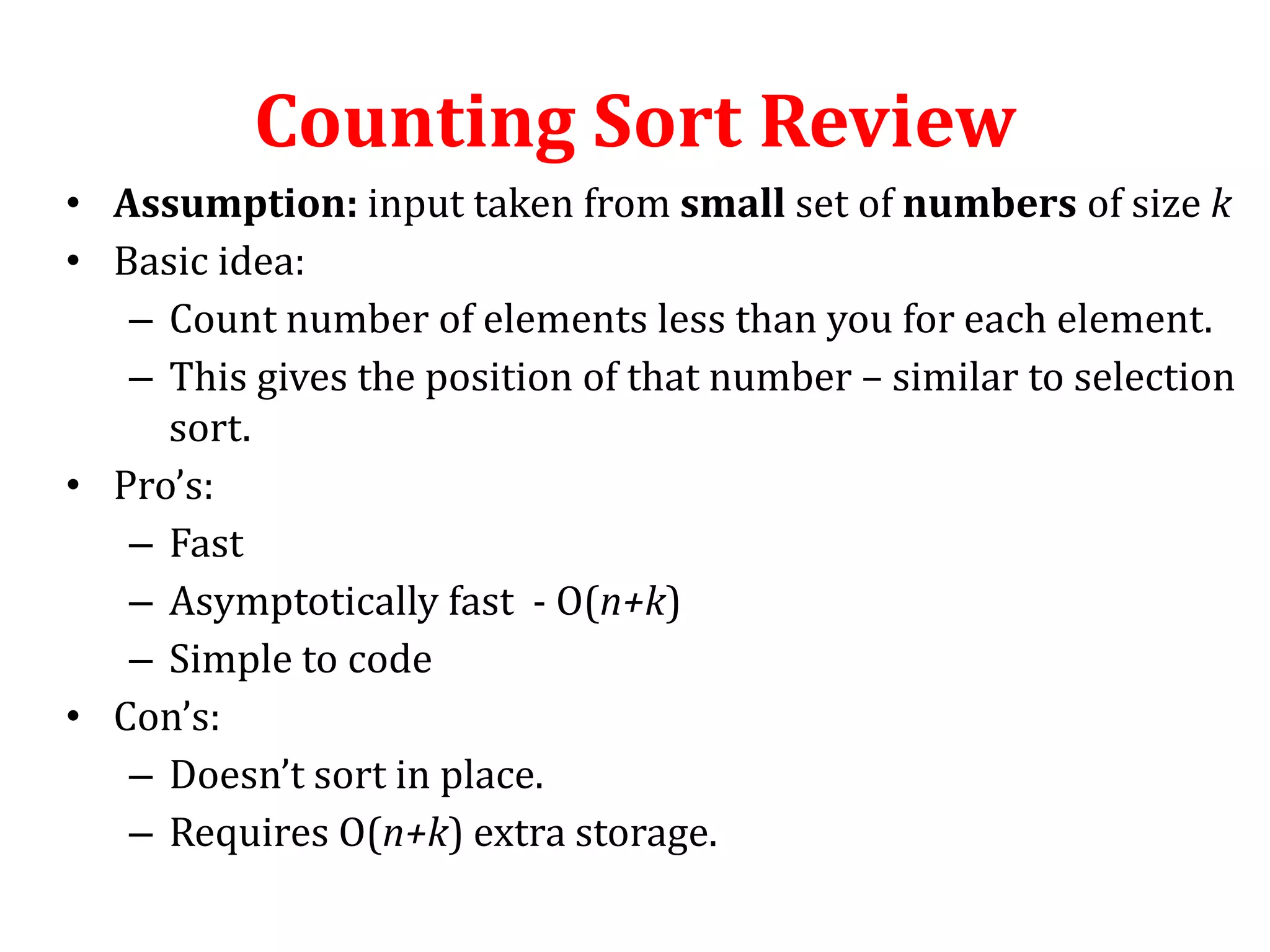
Addresses the conditions under which Counting Sort is applicable and discusses its pros and cons.
Acknowledges the presenter, MD. Shakhawat Hossain, a Computer Science student at the University of Rajshahi.


![Data Structures - Lecture 8 [Sorting Algorithms]](https://cdn.slidesharecdn.com/ss_thumbnails/lecture-8sortingalgorithms-150205105023-conversion-gate02-thumbnail.jpg?width=600ounds&width=560&fit=bounds)


