Download to read offline


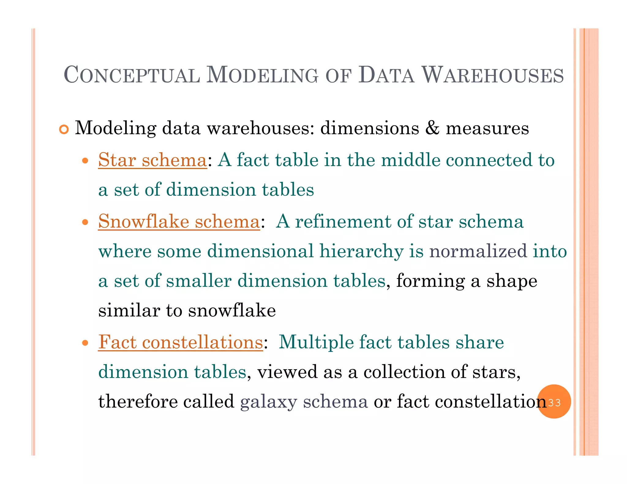
![DATA TRANSFORMATION: NORMALIZATION
Min-max normalization: to [new_minA, new_maxA]
i
Ex. Let income range $12,000 to $98,000 normalized to [0.0,
AAA
AA
A
minnewminnewmaxnew
minmax
minv
v _)__('
g , , [ ,
1.0]. Then $73,000 is mapped to
Z-score normalization (μ: mean, σ: standard deviation):
716.00)00.1(
000,12000,98
000,12600,73
Ex Let μ = 54 000 σ = 16 000 Then 2251
000,54600,73
A
Av
v
'
Ex. Let μ = 54,000, σ = 16,000. Then
Normalization by decimal scaling
225.1
000,16
v
v' Where j is the smallest integer such that Max(|ν’|) < 1 22j
v
10
' Where j is the smallest integer such that Max(|ν |) < 1](https://image.slidesharecdn.com/cs501datapreprocessingdw-180604113047/85/Cs501-data-preprocessingdw-22-320.jpg)


![DATA TRANSFORMATION: NORMALIZATION
Min-max normalization: to [new_minA, new_maxA]
i
Ex. Let income range $12,000 to $98,000 normalized to [0.0,
AAA
AA
A
minnewminnewmaxnew
minmax
minv
v _)__('
g , , [ ,
1.0]. Then $73,000 is mapped to
Z-score normalization (μ: mean, σ: standard deviation):
716.00)00.1(
000,12000,98
000,12600,73
Ex Let μ = 54 000 σ = 16 000 Then 2251
000,54600,73
A
Av
v
'
Ex. Let μ = 54,000, σ = 16,000. Then
Normalization by decimal scaling
225.1
000,16
v
v' Where j is the smallest integer such that Max(|ν’|) < 1 22j
v
10
' Where j is the smallest integer such that Max(|ν |) < 1](https://image.slidesharecdn.com/cs501datapreprocessingdw-180604113047/75/Cs501-data-preprocessingdw-22-2048.jpg)


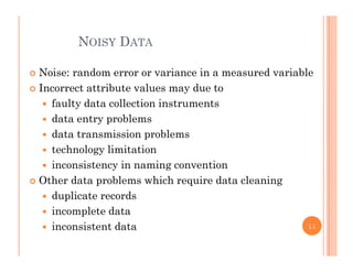
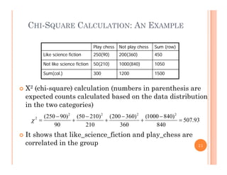
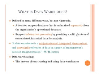
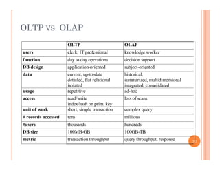
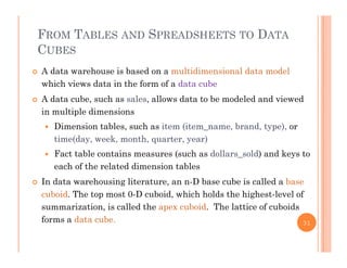
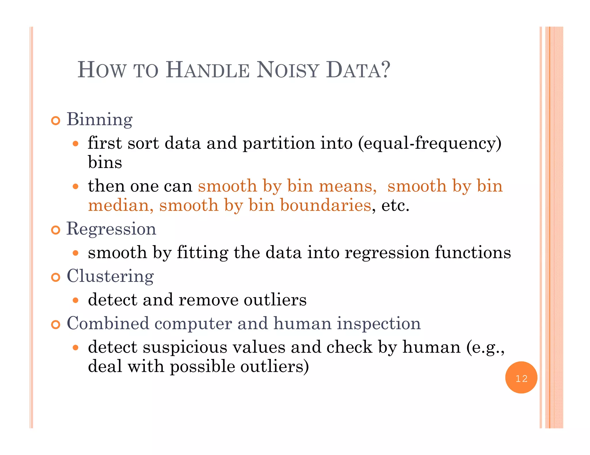
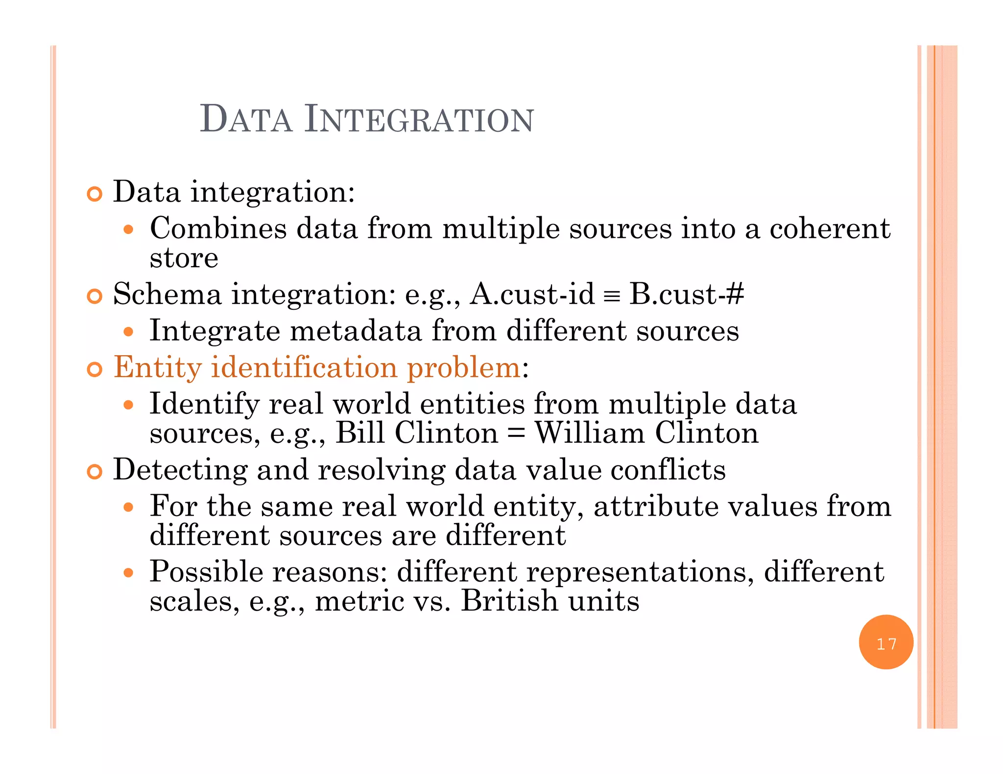
This document discusses data preprocessing and data warehouses. It explains that real-world data is often dirty, incomplete, noisy, and inconsistent. Data preprocessing aims to clean and transform raw data into a format suitable for data mining. The key tasks of data preprocessing include data cleaning, integration, transformation, reduction, and discretization. Data cleaning involves techniques like handling missing data, identifying outliers, and resolving inconsistencies. Data integration combines data from multiple sources. The document also defines characteristics of a data warehouse such as being subject-oriented, integrated, time-variant, and nonvolatile.


