Download to read offline

![WHAT IS FREQUENT PATTERN
ANALYSIS?
Frequent pattern: a pattern (a set of items, subsequences, substructures,
etc.) that occurs frequently in a data set
First proposed by Agrawal, Imielinski, and Swami [AIS93] in the context
of frequent itemsets and association rule mining
Motivation: Finding inherent regularities in data
What products were often purchased together?— Beer and diapers?!
What are the subsequent purchases after buying a PC?
What kinds of DNA are sensitive to this new drug?
Can we automatically classify web documents?
Applications
Basket data analysis, cross-marketing, catalog design, sale campaign
analysis, Web log (click stream) analysis, and DNA sequence analysis.
2](https://image.slidesharecdn.com/cs501miningfrequentpatterns-180604113052/85/Cs501-mining-frequentpatterns-2-320.jpg)

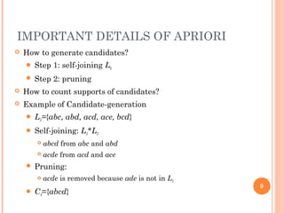
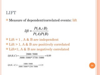
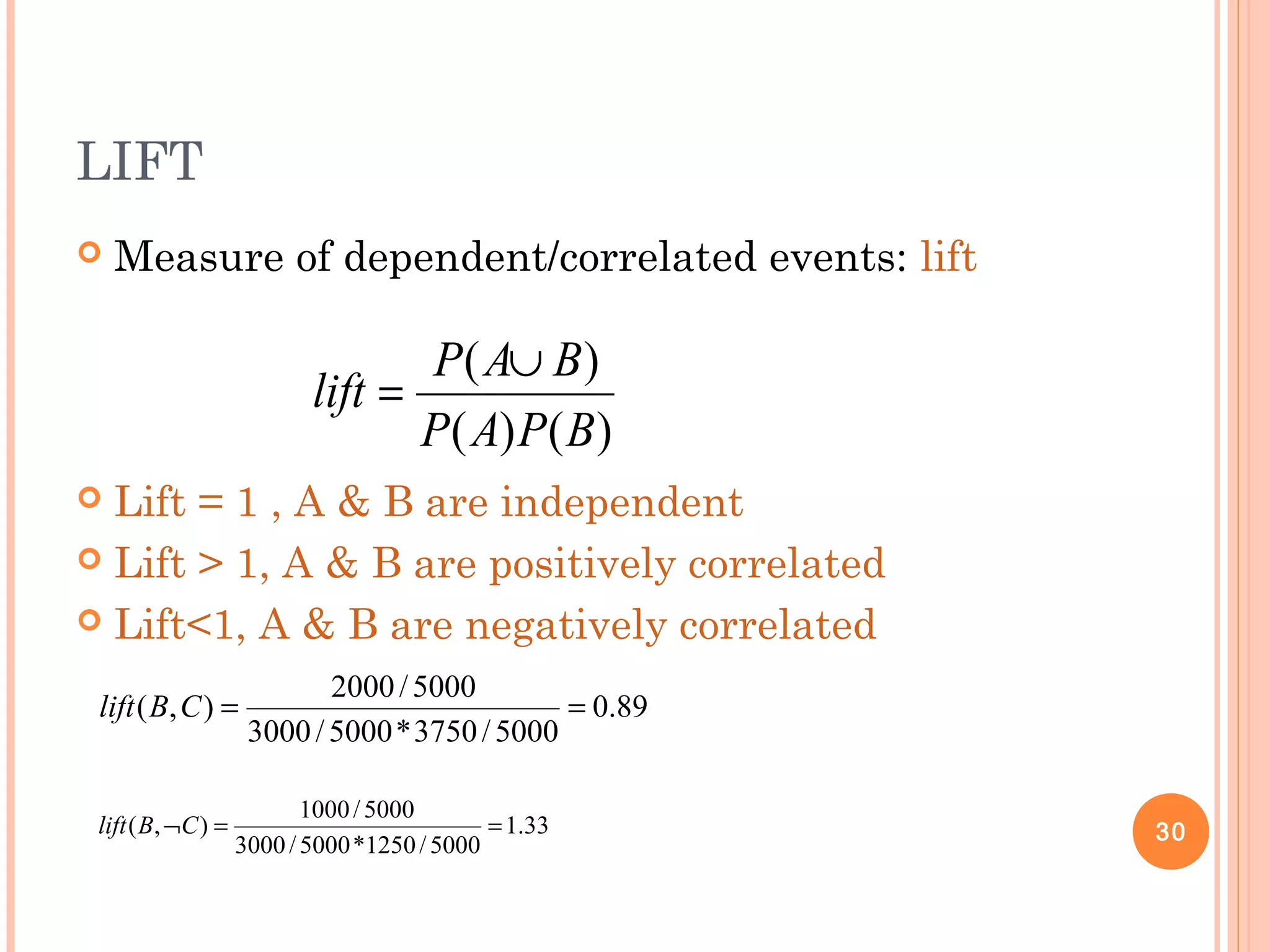
![INTERESTINGNESS MEASURE: CORRELATIONS
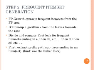
(LIFT)
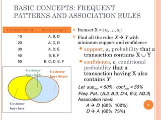
play basketball ⇒ eat cereal [40%, 66.7%] is misleading
The overall % of students eating cereal is 75% > 66.7%.
play basketball ⇒ not eat cereal [20%, 33.3%] is more accurate,
although with lower support and confidence
29
Basketball Not basketball Sum (row)
Cereal 2000 1750 3750
Not cereal 1000 250 1250
Sum(col.) 3000 2000 5000](https://image.slidesharecdn.com/cs501miningfrequentpatterns-180604113052/85/Cs501-mining-frequentpatterns-29-320.jpg)
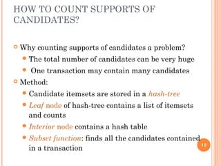
![WHAT IS FREQUENT PATTERN
ANALYSIS?
Frequent pattern: a pattern (a set of items, subsequences, substructures,
etc.) that occurs frequently in a data set
First proposed by Agrawal, Imielinski, and Swami [AIS93] in the context
of frequent itemsets and association rule mining
Motivation: Finding inherent regularities in data
What products were often purchased together?— Beer and diapers?!
What are the subsequent purchases after buying a PC?
What kinds of DNA are sensitive to this new drug?
Can we automatically classify web documents?
Applications
Basket data analysis, cross-marketing, catalog design, sale campaign
analysis, Web log (click stream) analysis, and DNA sequence analysis.
2](https://image.slidesharecdn.com/cs501miningfrequentpatterns-180604113052/75/Cs501-mining-frequentpatterns-2-2048.jpg)


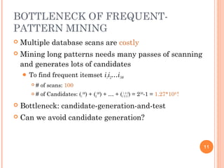
![INTERESTINGNESS MEASURE: CORRELATIONS
(LIFT)
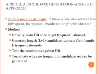
play basketball ⇒ eat cereal [40%, 66.7%] is misleading
The overall % of students eating cereal is 75% > 66.7%.
play basketball ⇒ not eat cereal [20%, 33.3%] is more accurate,
although with lower support and confidence
29
Basketball Not basketball Sum (row)
Cereal 2000 1750 3750
Not cereal 1000 250 1250
Sum(col.) 3000 2000 5000](https://image.slidesharecdn.com/cs501miningfrequentpatterns-180604113052/75/Cs501-mining-frequentpatterns-29-2048.jpg)

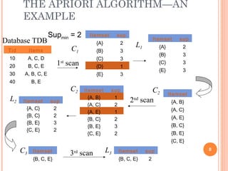
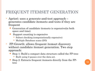
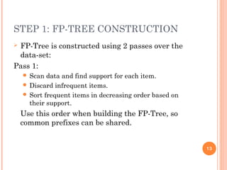
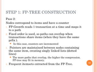
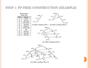
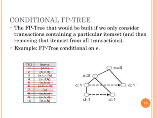
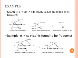
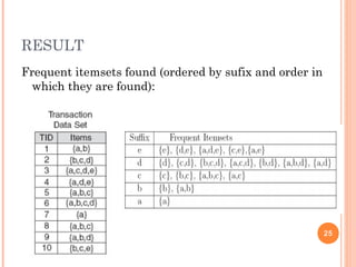
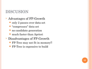
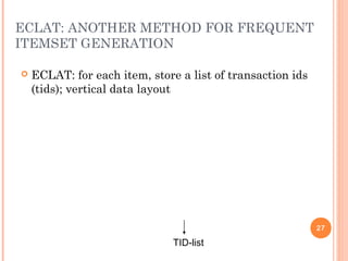
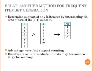
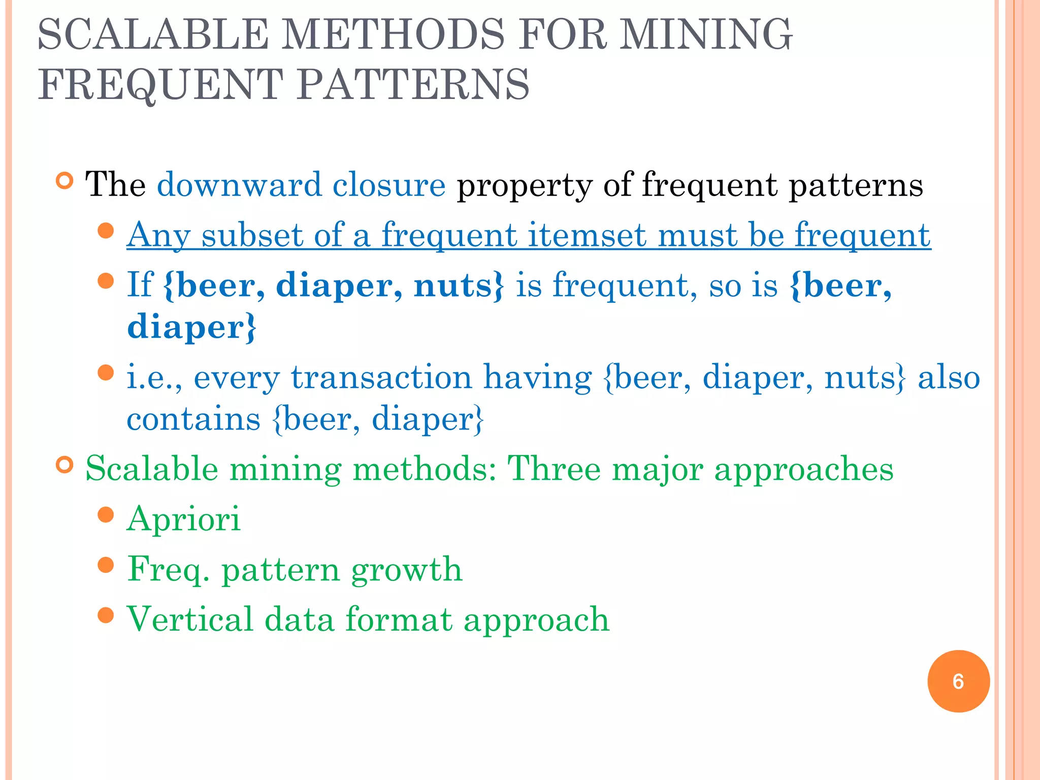
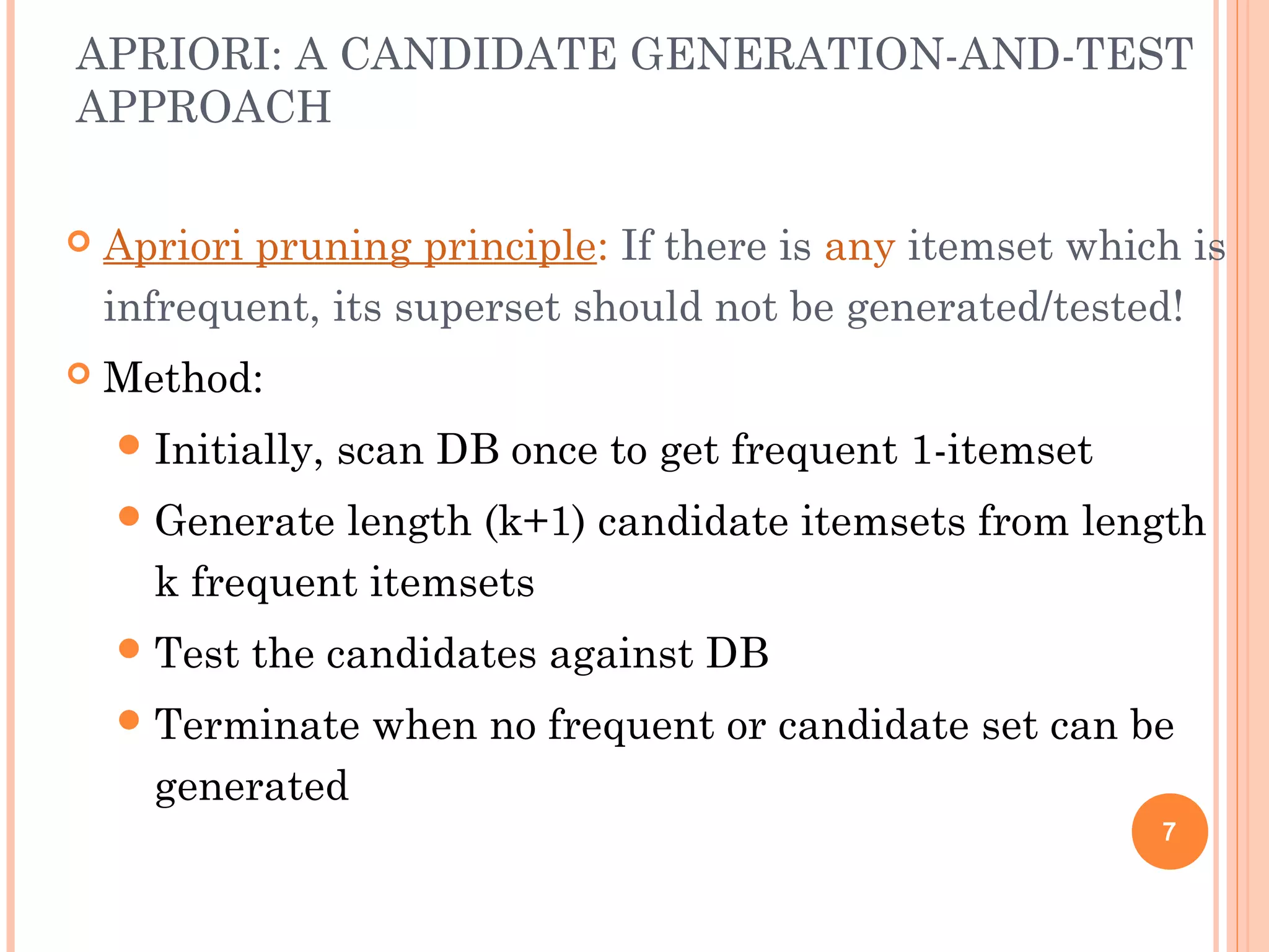
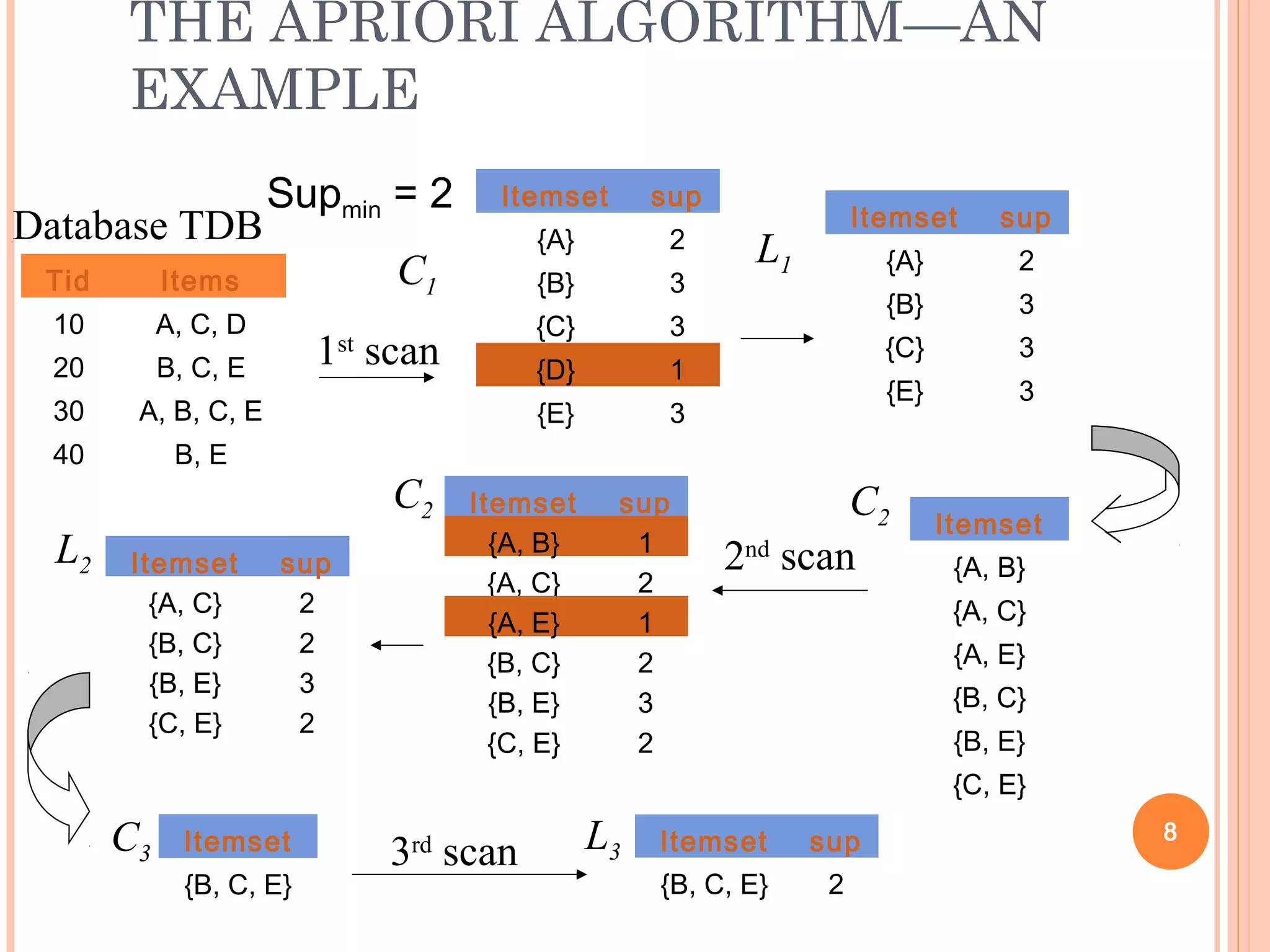
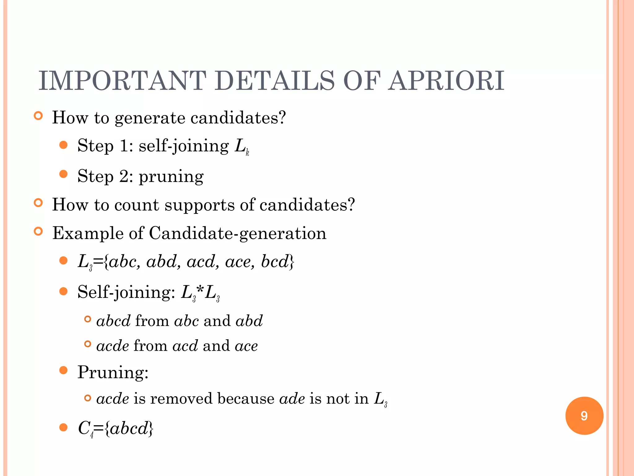
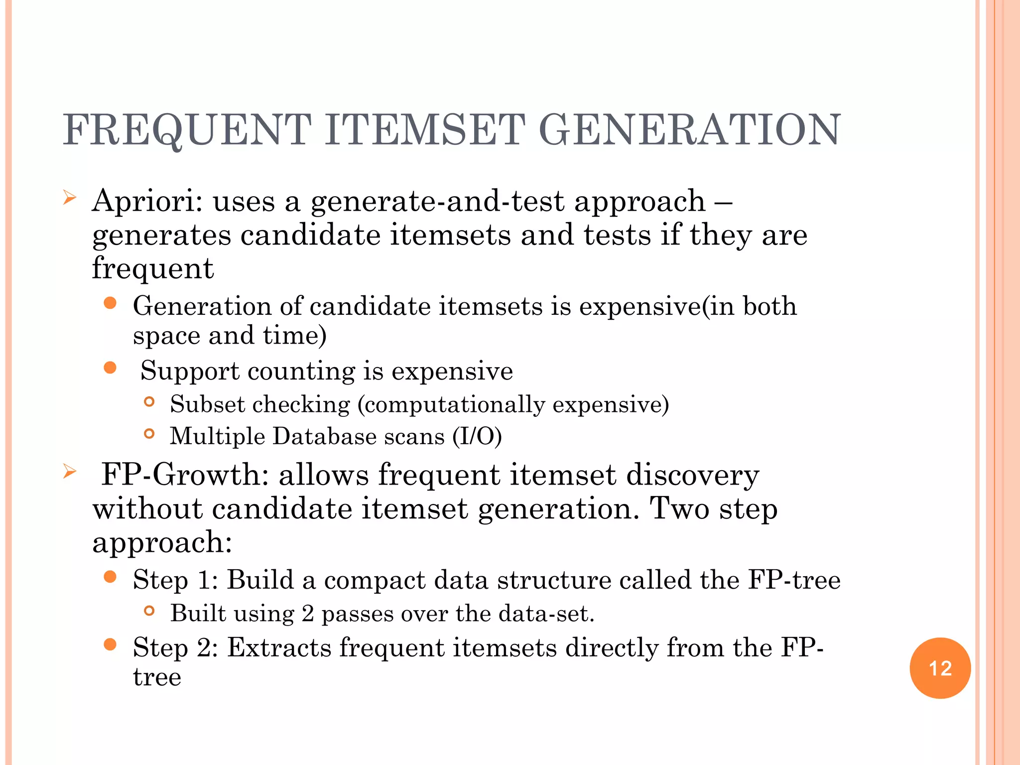
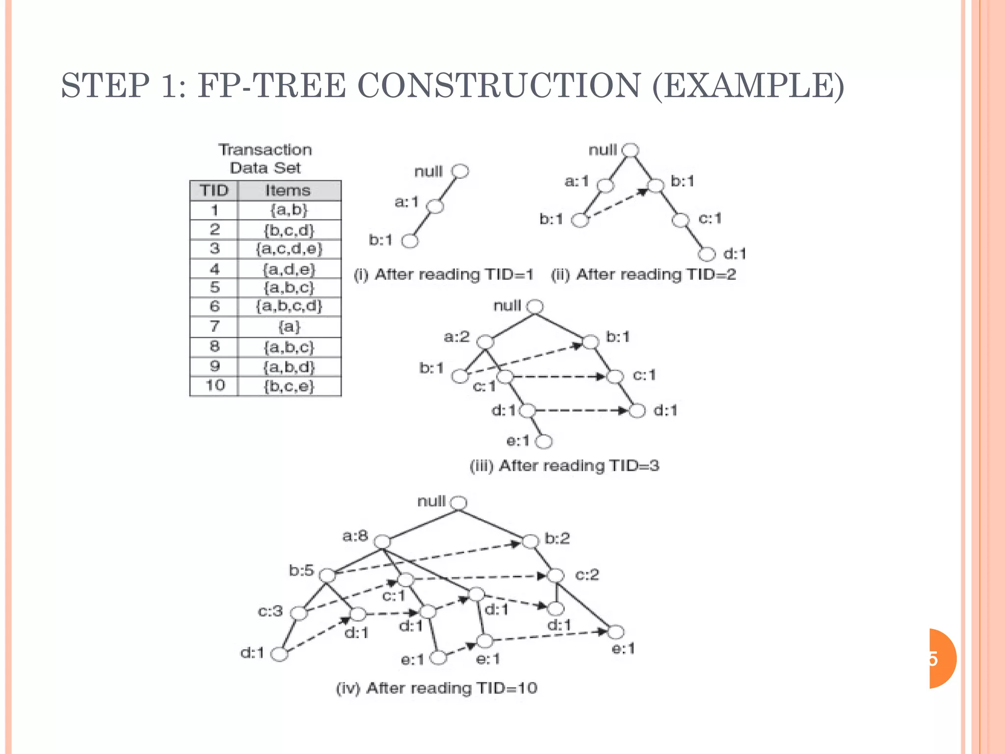
Frequent pattern mining aims to discover patterns that occur frequently in a dataset. It finds inherent regularities without any preconceptions. The frequent patterns can then be used for applications like association rule mining, classification, clustering, and more. Two major approaches for mining frequent patterns are the Apriori algorithm and FP-Growth. Apriori is a generate-and-test method while FP-Growth avoids candidate generation by building a compact data structure called an FP-tree to extract patterns directly.


