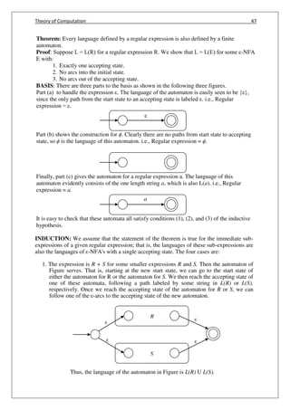
The document is a comprehensive educational resource on the Theory of Computation, authored by G. Appasami. It covers various topics including finite automata, grammars, pushdown automata, Turing machines, and unsolvable problems, structured into multiple units with specific objectives for students. The document contains acknowledgments, bibliography, and detailed explanations of mathematical proofs and concepts relevant to computational theory.


![Theory of Computation 3
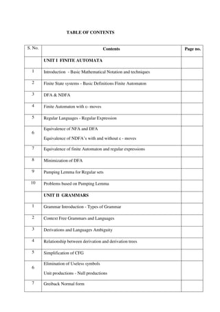
Let n = k + 1, P(k + 1) = 42(k + 1) + 1
+ 3(k + 1) + 2
= 42(k + 1) + 1
+ 3(k + 1) + 2
= 42k + 2 + 1
+ 3k + 1 + 2
= 42k + 1 + 2
+ 3k + 2 + 1
= 42k + 1.
42
+ 3k + 2.
31
= 42
.42k + 1
+ 3.3k + 2
= 42
.42k + 1
+ 42
3k+2
- 42
3k+2
+ 3.3k + 2
{ Add & Sub 42
3k+2
}
= 42
(42k + 1
+ 3k+2
) + 3k+2
(-42
+ 3)
= 42
(13.t)- 3k+2
(-42
+ 3) { 42k + 1
+ 3k + 2
= 13.t}
= 16 (13.t)- 3k+2
(-13)
= 13[16. t + 3k+2
]
= Multiple of 13
P(k + 1) is multiple of 13, Hence proved.
Example 2
Prove 1 + 2 + 3 + … + n = n (n+1)/2 using induction method.
Proof:
Let n = 1, then LHS = 1 and RHS = 1 (1 + 1) / 2 = 1
LHS = RHS
Let n = 2, then LHS = 1 + 2 = 3 and RHS = 2(2 + 1) / 2 = 3
LHS = RHS
Let n = k, 1 + 2 + 3 + … + k = k (k+1)/2
Consider n = k +1, then LHS = 1 + 2 + 3 + … + k + (k+1) = (k+1) (k+2) / 2
RHS = k (k+1)/2 + (k + 1)
= k2
+ k + 2 (k + 1)
2 2
= (k2
+ 3k + 2) / 2
= (k+1) (k+2) / 2
LHS = RHS
Hence Proved.
Example 3
Show that 2n
> n3
for n ≥ 10 by mathematical induction.
Proof:
Let n= 10, 210
> 103
, 1024 > 1000, The condition is true.](https://image.slidesharecdn.com/cs6503theoryofcomputationbookv1-170609034600/85/Cs6503-theory-of-computation-book-notes-11-320.jpg)
![Theory of Computation 5
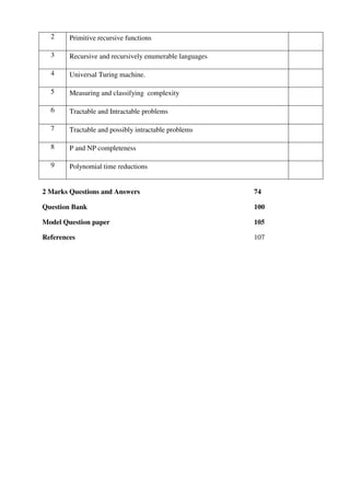
Example 4
Prove by mathematical induction Ʃn2
=
+ +
for all n ≥ 1.
Proof:
12
+ 22
+ ... + n2
=
+ +
Let n = 1, LHS = 12
= 1, RHS =
+ . +
=
𝑥 𝑥
= 1, LHS = RHS
Let n = 2, LHS = 12
+ 22
= 1 + 4 = 5, RHS =
+ . +
=
𝑥 𝑥
= 5, LHS = RHS
Let n = k, 12
+ 22
+ ... + k2
=
+ +
, assumed to be true
Let n = k+1, LHS = 12
+ 22
+ ... + k2
+ (k + 1)2
=
+ +
+ (k + 1)2
=
+ +
+ (k + 1) (k +1)
=
+ +
+
+ +
=
+ + + + +
=
+ [ + + + ]
=
+ ( 2+ + + )
=
+ ( 2+ + )
=
+ + +
RHS =
+ + + [ + ]+
=
+ + + +
=
+ + +
LHS = RHS, Hence Proved](https://image.slidesharecdn.com/cs6503theoryofcomputationbookv1-170609034600/85/Cs6503-theory-of-computation-book-notes-13-320.jpg)
![Theory of Computation 6
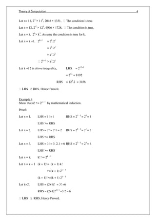
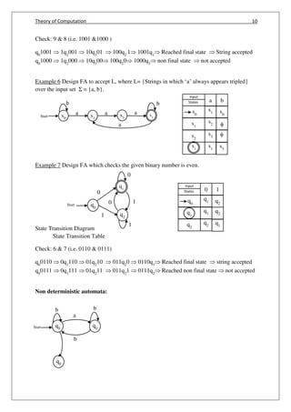
Alphabets, Strings and language
Alphabet:
An alphabet is a finite non empty set of symbols. The symbol Σ is used to denote the
alphabet.
1) Σ = {0, 1}
2) Σ = {a, b, c, …, z}
3) Σ = Set of ASII character
String:
A string is a finite sequence of symbols chosen from some alphabet.
1) Σ ={0,1} 11001 [ Empty string is denoted by ]
2) Σ = {a, b, c} aabbcbbbaa
The total number of symbols in the string is called length of the string
Example:
1) |0001|=4
2) |100|=3
Empty string ( ):
Empty string is the string with zero occurrence of symbol .This empty string is denote
by
Power of an alphabet
If Σ is an alphabet, then the set of all string of certain length forms an alphabet .
Σk
to be the set of string of length k for each symbol in Σ.
Example :
∑ = {0, 1}
∑ ={ }
∑ = {0, 1}
∑ = {00, 01, 10, 11}
∑ = {000, 001, 010, 011, 100, 101, 110, 111}](https://image.slidesharecdn.com/cs6503theoryofcomputationbookv1-170609034600/85/Cs6503-theory-of-computation-book-notes-14-320.jpg)
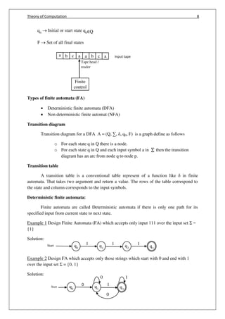
![Theory of Computation 7
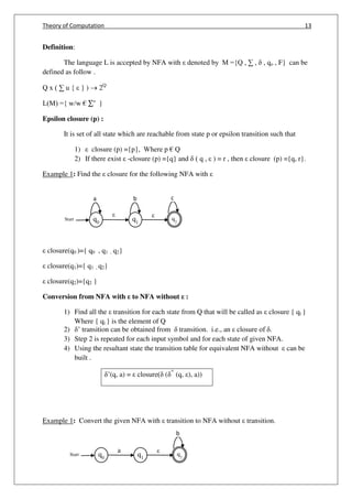
∑+
= ∑ 𝑈 ∑ 𝑈 ∑ …
∑+
= ∑ ⋃∞
=
∑∗
= ∑ 𝑈 ∑ 𝑈 ∑ 𝑈 …
∑∗
= ∑ ⋃∞
=
Set of all strings over an alphabet is denoted by ∑∗
Set of all strings over an alphabet except null string is denoted by ∑+
Concatination of strings
Let X and Y be the two strings over Σ = {a, b, c}. Then XY denotes the concatenation
of X and Y.
X = aabb
Y = cccc
XY = aabbcccc
YX = ccccaabb
Language [Language is a collection of all strings]
A set of strings of all which are chosen from ∑∗
is called a language, where ∑ is a
particular alphabet set.
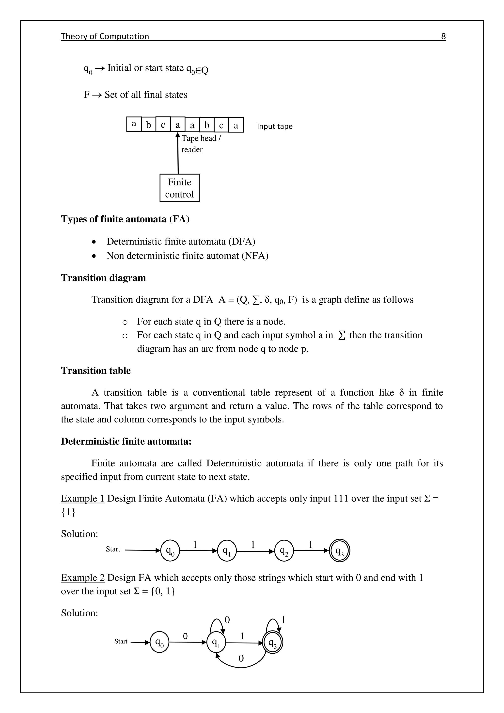
Finite state system (or) finite automata :
A finite automata has a several parts. It has set of states and rules for moving from
one state to another state depending on the input symbols.
It has the input alphabet, start state, and a set of accept state.
Definition of finite automata:
A finite automata is a collection of 5-tuples A = (Q , ∑, , q0
, F)
Where A Name of the finite automata
Q Finite set of states [non-empty]
∑ The set of input symbols [input set]
The transition function [Move from one state to another ] :Qx ΣQ](https://image.slidesharecdn.com/cs6503theoryofcomputationbookv1-170609034600/85/Cs6503-theory-of-computation-book-notes-15-320.jpg)


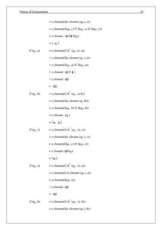
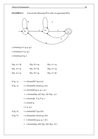
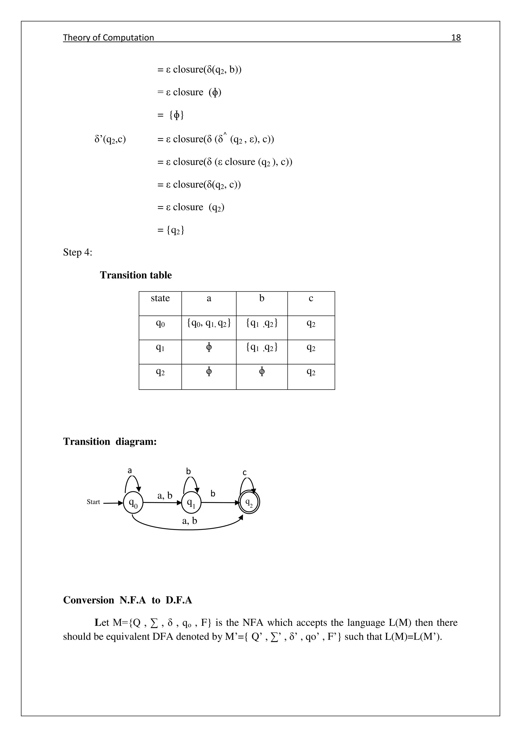
![Theory of Computation 19
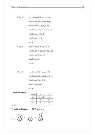
Conversion Steps:
STEP 1: The start state of NFA M will be the start state of DFA M’. Hence add qo of NFA to
Q’ then, find the transition for this start state.
STEP 2: For each state {q1, q2, q3……qi} in Q’. The transition for each input symbol ∑ can
be obtained as follows,
(i) ’( [q1,q2,q3……qi], a) = (q1,a ) U (q2, a)…… U (qi, a)
= [q1, q2, q3, ... , qk]
(ii) Add the [q1, q2, q3, ... , qk] in DFA if it is not already in Q.
(iii) Then, find the transition for every input symbol from ∑ for states [q1, q2,
q3, ... , qk], if we get some state [q1,q2…..qn] which is not Q’ of DFA then add
this to Q’.
(iv) If there is no new state generating then stop the process after finding all
the transition.
(v) For the state [q1, q2, q3, ... , qk] € Q’ of DFA, if any 1 state qi is a final
state of NFA then [q1,q2…..qn] becomes a final state. Thus the set of all final
states € F’ of DFA.
Example 1: Construct the equivalent DFA for the given NFA.
M = ({q0, q1}, {0,1}, , qo, {q1}) where is given by
(q0,0) = {q0, q1}
(q0,1) = { q1}
(q1,0) = φ
(q1,0) = {q0, q1}
Sol:
Transition Table (NFA)
St/Ip 0 1
q0 {q0, q1} {q1}
q1 φ {q0, q1}](https://image.slidesharecdn.com/cs6503theoryofcomputationbookv1-170609034600/85/Cs6503-theory-of-computation-book-notes-27-320.jpg)

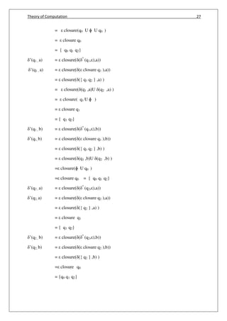
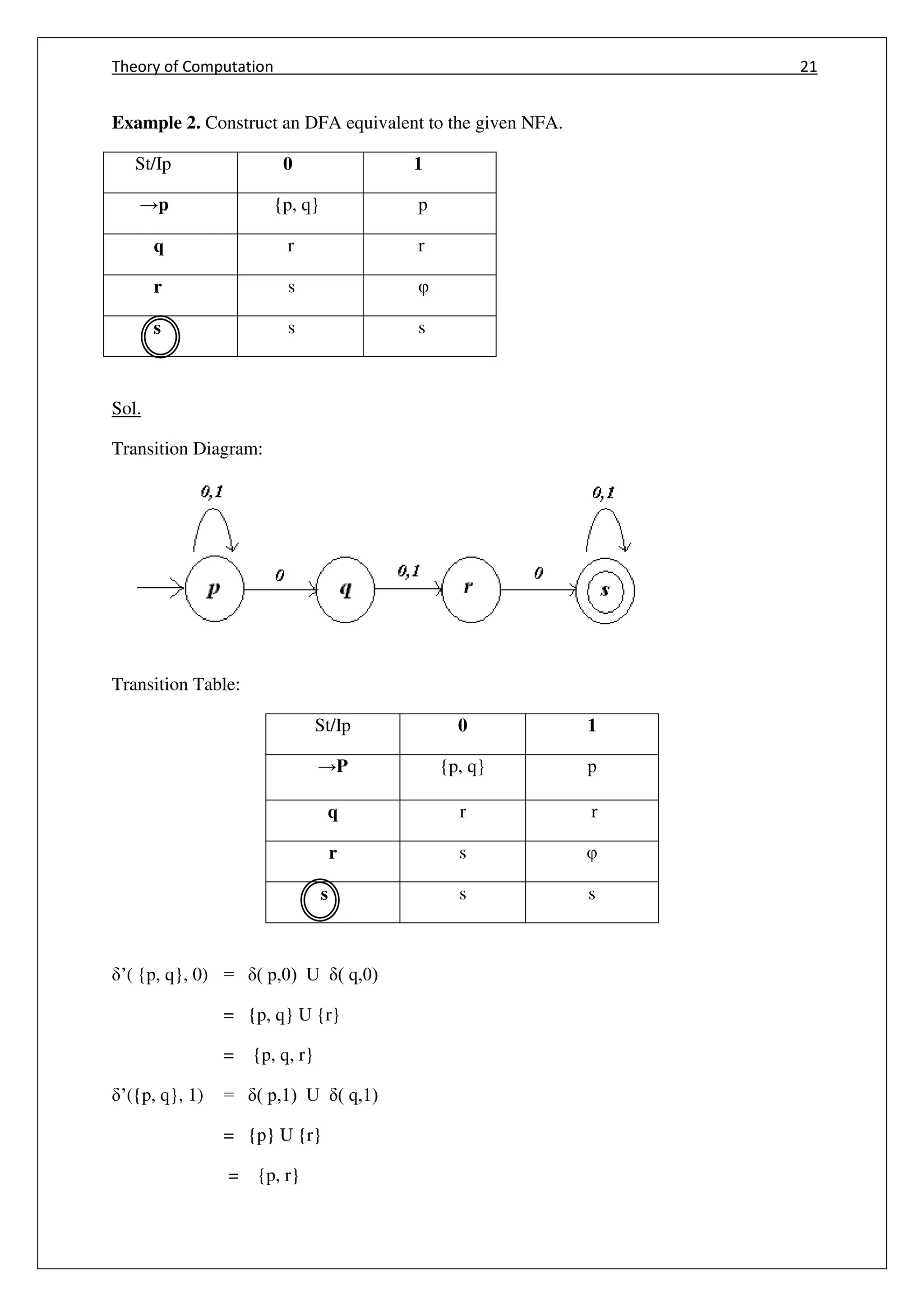
![Theory of Computation 23
q
{p, q} {p, q, r} {p, r}
{p, q, r} {p, q, r, s} {p, r}
{p, r} {p, q, s} p
’({p, q, r, s}, 0) = ( p,0) U ( q,0) U ( r,0) U ( s,0)
= {p,q} U {r} U {s} U {s}
= {p, q, r, s}
’({p, q, r, s}, 1) = ( p,1) U ( q,1) U ( r,1) U ( s,1)
= {p} U {r} U { φ } U {s}
= {p, r, s}
’( [p,q,s],0) = ( p,0) U ( q,0) U ( s,0)
= {p,q} U {r} U {s}
= {p, q, r, s}
’( [p,q,s],1) = ( p,1) U ( q,1) U ( s,1)
= {p,q} U {r} U {s}
= {p, q, r, s}
New transition table:
St/Ip 0 1
→P {p, q} p
q r r
r s φ
s s s
{p, q} {p, q, r} {p, r}
{p, q, r} {p, q, r, s} {p, r}
{p, r} {p, q, s} p
{p,q,r,s} {p, q, r, s} {p, r, s}](https://image.slidesharecdn.com/cs6503theoryofcomputationbookv1-170609034600/85/Cs6503-theory-of-computation-book-notes-31-320.jpg)
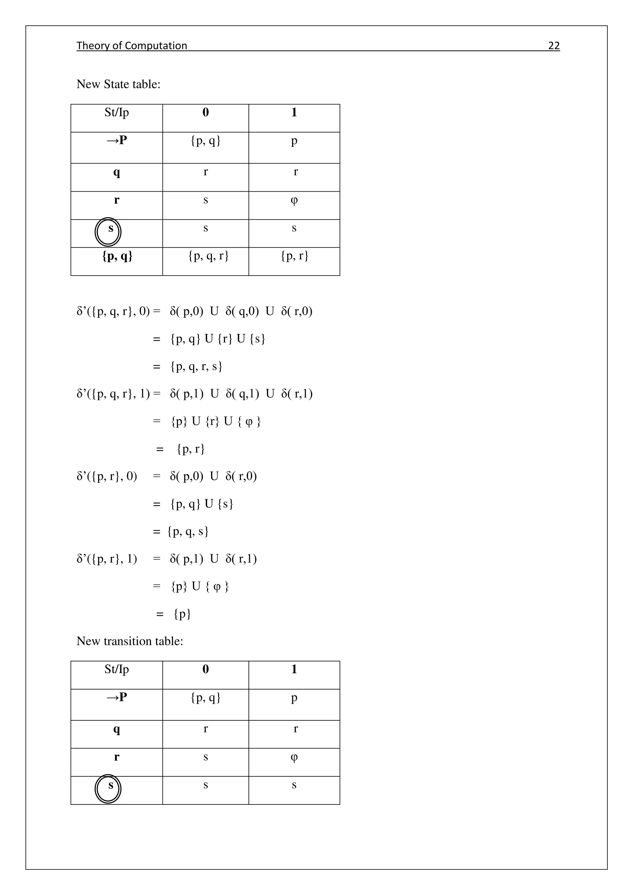
![Theory of Computation 24
q2
{p,q,s} {p, q, r, s} {p, r, s}
’({p, r, s}, 0) = ( p,0) U ( r,0) U ( s,0)
= {p,q} U {s} U {s}
= {p, q, s},
’({p, r, s}, 1) = ( p,1) U ( r,1) U ( s,1)
= {p} U {s} U {s}
= {p, s}
New transition table:
St/Ip 0 1
→[P] [p,q] [ p]
[q] [r] [ r]
[r] [s] φ
s [s] [s]
[p,q] [p,q,r] [p,r]
[p,q,r] [p,q,r,s] [p,r]
[p,r] [p,q,s] [p]
p,q,r,s [p,q,r,s] [p,r,s]
p,q,s [p,q,r,s] [p,r,s]
p,r,s [p,q,s] [p,s]
’( [p,s],0) = ( p,0) U ( s,0)
= {p,q} U {s}
= [p,q,s]
’( [p,s],1) = ( p,1) U ( s,1)
= {p} U {s}
= [p,s]](https://image.slidesharecdn.com/cs6503theoryofcomputationbookv1-170609034600/85/Cs6503-theory-of-computation-book-notes-32-320.jpg)
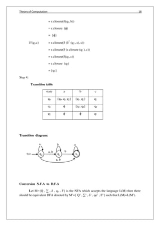
![Theory of Computation 25
New transition table:
Transition Diagram: (DFA)
METHOD FOR CONVERSION NFA WITH TO DFA
Step 1 : Consider M={Q, ∑, , q0, F} is a NFA with , we have to convert this NFA with to
equivalent DFA,
MD =( QD,∑ D, D, qD, FD). Obtain closure (q0 ) = { p1p2……pn } becomes its start
state of DFA.
Step2 : Obtain transition on { p1p2……pn } for each input.
D ({ p1p2……pn }, a) = closure( (P1 ,a) U (P2 (a) U ……U(Pn ,a))
=⋃ closure Pi , a= where a ϵ ∑
Step3 : State obtained [ P1P2……Pn ] ϵ QD , states containing final state Pi is a final state
DFA.
St/Ip 0 1
→[P] [p,q] [ p]
[q] [r] [ r]
[r] [s] -
[s] [s] [s]
[p,q] [p,q,r] [p,r]
[p,q,r] [p,q,r,s] [p,r]
[p,r] [p,q,s] [p]
[p,q,r,s] [p,q,r,s] [p,r,s]
[p,q,s] [p,q,r,s] [p,r,s]
[p,r,s] [p,q,s] [p,s]
[p,s] [p,q,s] [p,s]](https://image.slidesharecdn.com/cs6503theoryofcomputationbookv1-170609034600/85/Cs6503-theory-of-computation-book-notes-33-320.jpg)
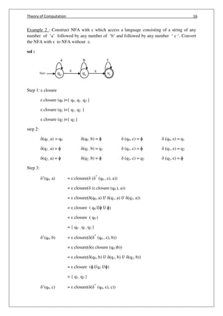
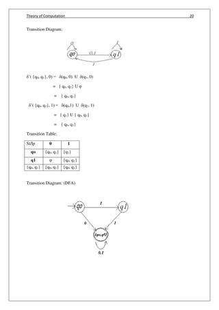
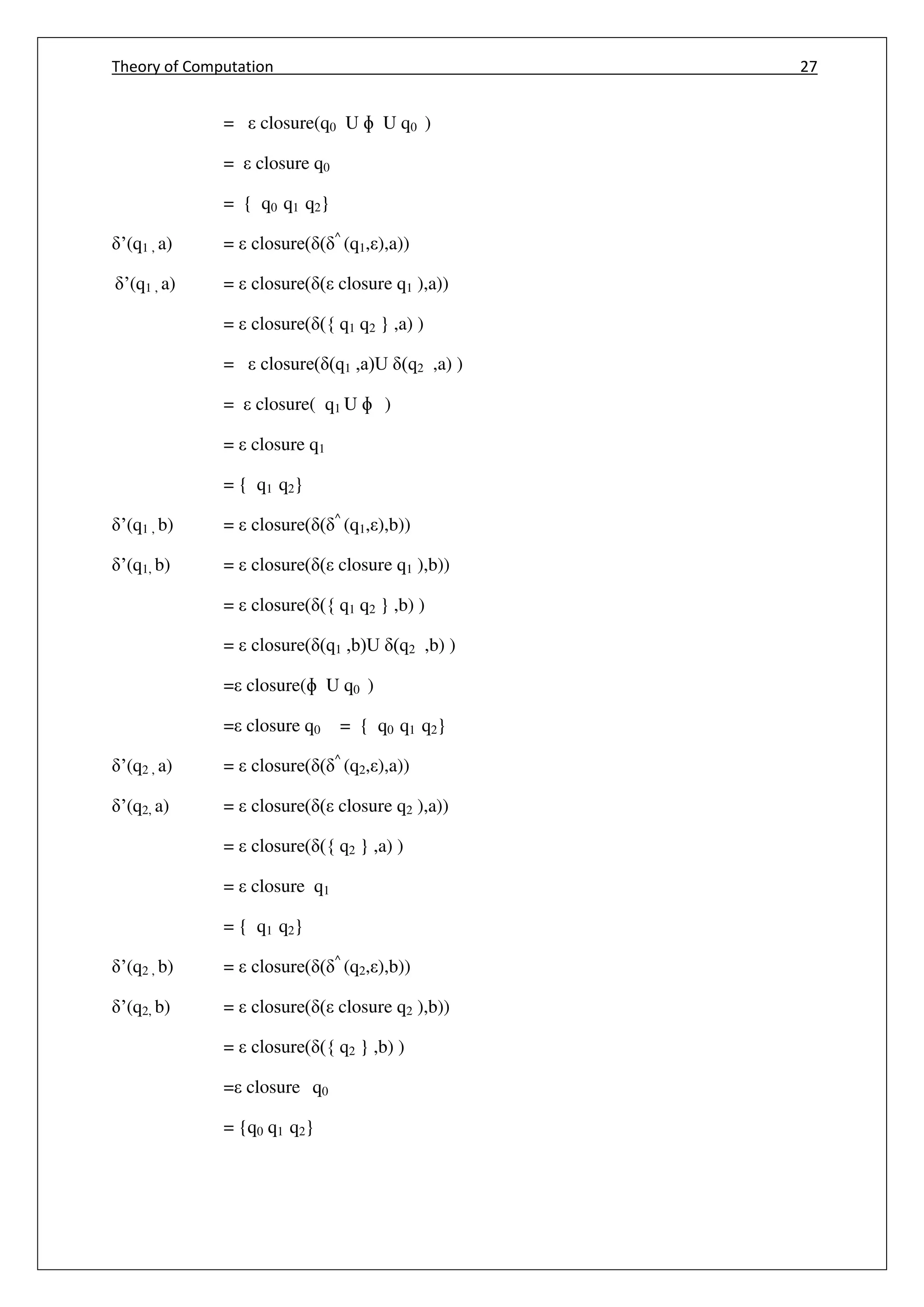
![Theory of Computation 28
q0
q2
11
Start
a,b
a,b
q1
a,b
a,b
a,b
a,bbb
b
Transition of NFA
input
state
a b
q0 { q1 q2} {q0 q1 q2}
q1 { q1 q2} {q0 q1 q2}
q2 { q1 q2} {q0 q1 q2}
Transition diagram
‘([q1 q2 ],a)= (q1 ,a) U (q2,a)
= { q1 , q2}U{ q1 , q2 }
=[ q1 , q2 ]
‘([q1 q2 ],b)= (q1 ,b) U (q2,b)
= { q0 , q1 , q2}U{ q0 , q1 , q2 }
=[q0 , q1 , q2 ]
‘([q0 q1 q2 ],a)= (q0 ,a) U (q1 ,a) U (q2,a)
={ q1 , q2}U{ q1 , q2 }U{ q1 , q2 }
=[ q1 , q2 ]
‘([q0 q1 q2 ],b)= (q0 ,b) U (q1 ,b) U (q2,b)
={ q0 ,q1 , q2}U{ q0 ,q1 , q2 }U{ q0 ,q1 , q2 }
=[ q0 ,q1 , q2 ]
Transition table for DFA](https://image.slidesharecdn.com/cs6503theoryofcomputationbookv1-170609034600/85/Cs6503-theory-of-computation-book-notes-36-320.jpg)
![Theory of Computation 29
[q1,q2,q3]
input
state
a b
q0 [ q1 q2 ] [ q0 q1 q2 ]
q1 [ q1 q2 ] [ q0 q1 q2 ]
q2 [ q1 q2 ] [ q0 q1 q2 ]
q1 q2 [ q1 q2 ] [ q0 q1 q2 ]
[ q0 q1 q2 ] [ q1 q2 ] [ q0 q1 q2 ]
a a b
a b b
b
a
a b
[q1,q2]
q0
q0 q1
q2](https://image.slidesharecdn.com/cs6503theoryofcomputationbookv1-170609034600/85/Cs6503-theory-of-computation-book-notes-37-320.jpg)
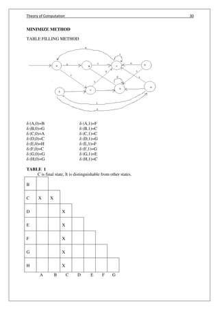

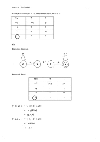
![Theory of Computation 34
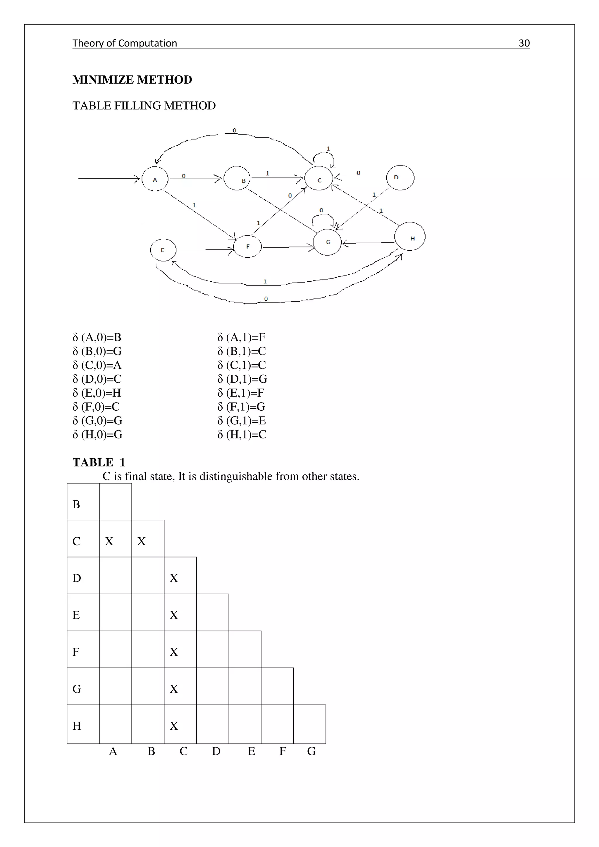
MINIMIZE METHOD [alter method]
𝜹(A,0)=B (A,1)=F
(B,0)=G (B,1)=C
(C,0)=A (C,1)=C
(D,0)=C (D,1)=G
(E,0)=H (E,1)=F
(F,0)= C (F,1)=G
(G,0)=G (G,1)=E
(H,0)=G (H,1)=c
Table 1
Stinput 0 1
A B F
B G C
C A C
D C G
E H/B F
F C G
G G E
H G C
B=H
Eliminate H
Replace H by B
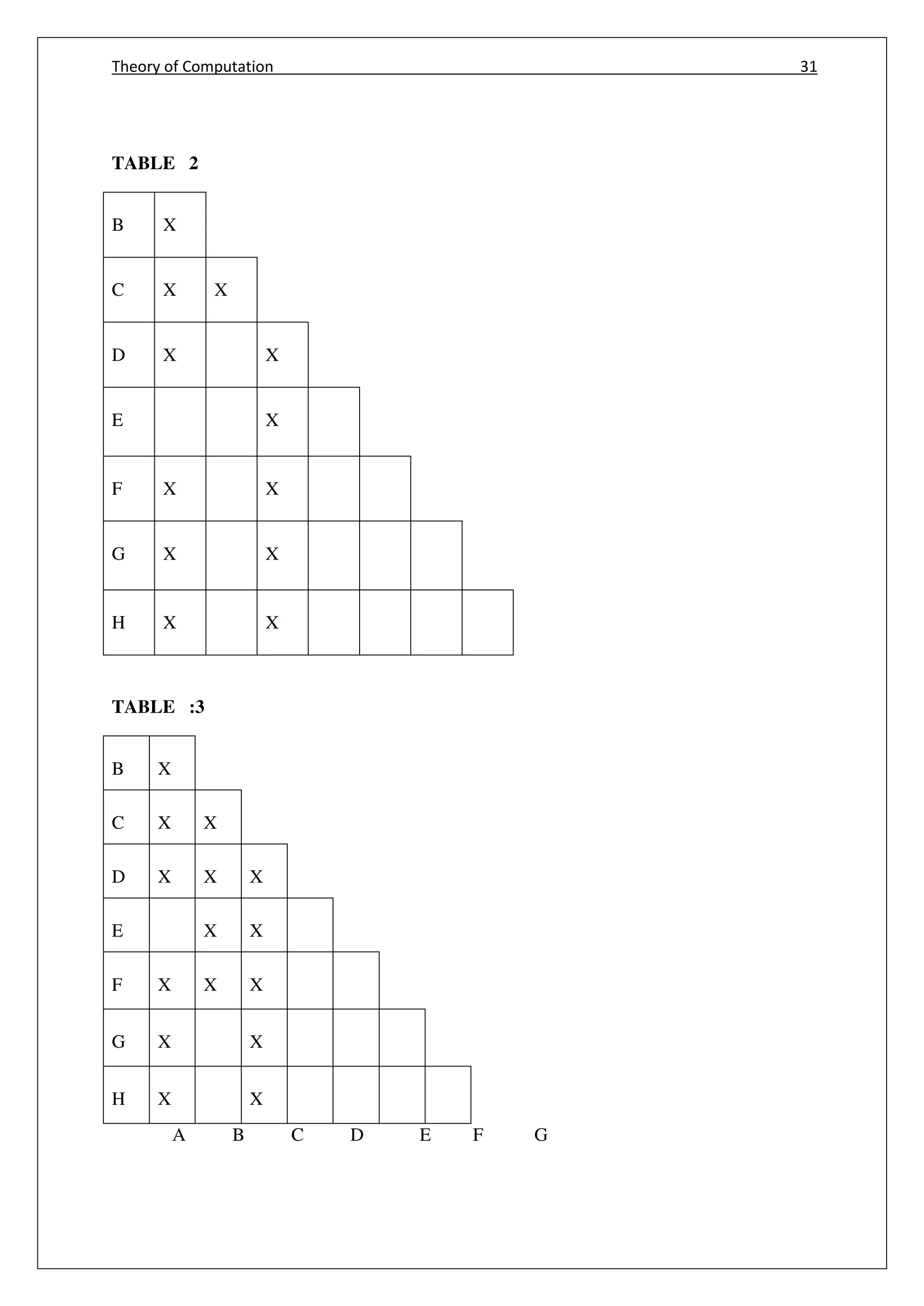
Table 2
St/input 0 1
A B F
B G C
C A C
D C G
E B F
F C G
G G E/A
A=E
Eliminate E
Replace E by A](https://image.slidesharecdn.com/cs6503theoryofcomputationbookv1-170609034600/85/Cs6503-theory-of-computation-book-notes-42-320.jpg)
![Theory of Computation 36
THEOREM: Let L be a set accepted by Nondeterministic finite automata (NFA), then there
exist a Deterministic finite automata (DFA) that accepts L.
Proof:
Let M = (Q, Σ, , qo, F) be an NFA for language L, then Define DFA Mʹ such that
Mʹ = (Qʹ, Σʹ, ʹ, qoʹ, Fʹ)
(i) The states of Mʹ are all the subsets of M then the Qʹ=2Q
(ii) The input symbols are common for both NFA and DFA. i.e., Σʹ = Σ
(iii) If q0 is the initial state in the NFA, then q0ʹ = [q0] = initial state in DFA
(iv) Fʹ be the set of all final states which contain final states of M. i.e., Fʹ ⊆ 2Q
∪ F
(v) The element in Qʹ will be denoted by [q1, q2, q3, … , qi] is a single state in Qʹ and the
elements in Q denoted by{q1, q2, q3, …, qi} are multiple states in Q. Define ʹ such that
ʹ([q1, q2, q3, …, qi], a) = [p1, p2, p3, …, pj] iff ʹ({q1, q2, q3, …, qi}, a) = {p1, p2, p3, …, pj}
This mean that in NFA, at the current states { q1, q2, q3, …, qi }, if we give input a
then it goes to the next states {p1, p2, p3, … , pj}.
While constructing DFA, the current state is assumed to be [q1, q2, q3, …, qi] with
input a, the next state is assumed to be [p1, p2, p3, … , pj].
On applying function on each of states q1, q2, q3, …, qi, the new states may be any
of the states from p1, p2, p3, … , pj.
The theorem can be proved by mathematical induction on length of the input string x.
ʹ(q0ʹ, x) = [q1, q2, q3, …, qi] if and only if (q0, x) = {q1, q2, q3, …, qi}
Basis: If the length of input string is 0, i.e., |x|=0, that means x is then q0ʹ = [q0]
Induction: If we assume that the hypothesis is true for the input string of length (or less
than ), then if xa is the string of length + .
Now the function ʹ can be written as ʹ(q0ʹ, xa) = ʹ( ʹ(q0, x), a)
By the induction hypothesis,
ʹ(q0ʹ, x) = [p1, p2, p3, … , pj] if and only if (q0, x) = {p1, p2, p3, … , pj}
By definition of ʹ
ʹ([p1, p2, … , pj], a) = [r1, r2, ..., rk] if and only if ({p1, p2, … , pj}, a) = {r1, r2, ..., rk}
Thus, ʹ(q0ʹ, xa) = [r1, r2, ..., rk] if and only if (q0, xa) = {r1, r2, ..., rk} is shown by induction.
Therefore L(M)=L(Mʹ).
i.e., If a language is accepted by NFA then the same language is also accepted by DFA.
Hence the theorem∎
THEOREM: If L is accepted by NFA with transition, then their exist L which is accepted
by NFA without transition. (Show that the language L accepted by NFA with move must
be accepted by NFA without move.)
Proof:
Let M = (Q, Σ, , q0, F) be an NFA with transition.
Construct Mʹ = (Q, Σ, ʹ, q0, Fʹ)
where Fʹ={ F ∪{q0} if closure contains state off
{ F otherwise
Mʹ is a NFA without moves. The ʹ function can be denoted by the ʹʹ with same input.
For example, ʹ(q, a) = ʹʹ(q, a) for some q in Q and a from Σ.
We will apply the method of induction with input string x.
Basis:
The x will not be because ʹ(q0, )={q0} and ʹʹ(q0, ) = -closure(q0)
Assume that the length of string x to be 1, i.e., |x|=1, then x is a symbol, say ʹaʹ.
ʹ(q0, a) = ʹʹ(q0, a)
Induction
Assume that the length of string x to be more than 1. i.e., |x| >1.](https://image.slidesharecdn.com/cs6503theoryofcomputationbookv1-170609034600/85/Cs6503-theory-of-computation-book-notes-44-320.jpg)


![Theory of Computation 3
Let n = k + 1, P(k + 1) = 42(k + 1) + 1
+ 3(k + 1) + 2
= 42(k + 1) + 1
+ 3(k + 1) + 2
= 42k + 2 + 1
+ 3k + 1 + 2
= 42k + 1 + 2
+ 3k + 2 + 1
= 42k + 1.
42
+ 3k + 2.
31
= 42
.42k + 1
+ 3.3k + 2
= 42
.42k + 1
+ 42
3k+2
- 42
3k+2
+ 3.3k + 2
{ Add & Sub 42
3k+2
}
= 42
(42k + 1
+ 3k+2
) + 3k+2
(-42
+ 3)
= 42
(13.t)- 3k+2
(-42
+ 3) { 42k + 1
+ 3k + 2
= 13.t}
= 16 (13.t)- 3k+2
(-13)
= 13[16. t + 3k+2
]
= Multiple of 13
P(k + 1) is multiple of 13, Hence proved.
Example 2
Prove 1 + 2 + 3 + … + n = n (n+1)/2 using induction method.
Proof:
Let n = 1, then LHS = 1 and RHS = 1 (1 + 1) / 2 = 1
LHS = RHS
Let n = 2, then LHS = 1 + 2 = 3 and RHS = 2(2 + 1) / 2 = 3
LHS = RHS
Let n = k, 1 + 2 + 3 + … + k = k (k+1)/2
Consider n = k +1, then LHS = 1 + 2 + 3 + … + k + (k+1) = (k+1) (k+2) / 2
RHS = k (k+1)/2 + (k + 1)
= k2
+ k + 2 (k + 1)
2 2
= (k2
+ 3k + 2) / 2
= (k+1) (k+2) / 2
LHS = RHS
Hence Proved.
Example 3
Show that 2n
> n3
for n ≥ 10 by mathematical induction.
Proof:
Let n= 10, 210
> 103
, 1024 > 1000, The condition is true.](https://image.slidesharecdn.com/cs6503theoryofcomputationbookv1-170609034600/75/Cs6503-theory-of-computation-book-notes-11-2048.jpg)

![Theory of Computation 5
Example 4
Prove by mathematical induction Ʃn2
=
+ +
for all n ≥ 1.
Proof:
12
+ 22
+ ... + n2
=
+ +
Let n = 1, LHS = 12
= 1, RHS =
+ . +
=
𝑥 𝑥
= 1, LHS = RHS
Let n = 2, LHS = 12
+ 22
= 1 + 4 = 5, RHS =
+ . +
=
𝑥 𝑥
= 5, LHS = RHS
Let n = k, 12
+ 22
+ ... + k2
=
+ +
, assumed to be true
Let n = k+1, LHS = 12
+ 22
+ ... + k2
+ (k + 1)2
=
+ +
+ (k + 1)2
=
+ +
+ (k + 1) (k +1)
=
+ +
+
+ +
=
+ + + + +
=
+ [ + + + ]
=
+ ( 2+ + + )
=
+ ( 2+ + )
=
+ + +
RHS =
+ + + [ + ]+
=
+ + + +
=
+ + +
LHS = RHS, Hence Proved](https://image.slidesharecdn.com/cs6503theoryofcomputationbookv1-170609034600/75/Cs6503-theory-of-computation-book-notes-13-2048.jpg)
![Theory of Computation 6
Alphabets, Strings and language
Alphabet:
An alphabet is a finite non empty set of symbols. The symbol Σ is used to denote the
alphabet.
1) Σ = {0, 1}
2) Σ = {a, b, c, …, z}
3) Σ = Set of ASII character
String:
A string is a finite sequence of symbols chosen from some alphabet.
1) Σ ={0,1} 11001 [ Empty string is denoted by ]
2) Σ = {a, b, c} aabbcbbbaa
The total number of symbols in the string is called length of the string
Example:
1) |0001|=4
2) |100|=3
Empty string ( ):
Empty string is the string with zero occurrence of symbol .This empty string is denote
by
Power of an alphabet
If Σ is an alphabet, then the set of all string of certain length forms an alphabet .
Σk
to be the set of string of length k for each symbol in Σ.
Example :
∑ = {0, 1}
∑ ={ }
∑ = {0, 1}
∑ = {00, 01, 10, 11}
∑ = {000, 001, 010, 011, 100, 101, 110, 111}](https://image.slidesharecdn.com/cs6503theoryofcomputationbookv1-170609034600/75/Cs6503-theory-of-computation-book-notes-14-2048.jpg)
![Theory of Computation 7
∑+
= ∑ 𝑈 ∑ 𝑈 ∑ …
∑+
= ∑ ⋃∞
=
∑∗
= ∑ 𝑈 ∑ 𝑈 ∑ 𝑈 …
∑∗
= ∑ ⋃∞
=
Set of all strings over an alphabet is denoted by ∑∗
Set of all strings over an alphabet except null string is denoted by ∑+
Concatination of strings
Let X and Y be the two strings over Σ = {a, b, c}. Then XY denotes the concatenation
of X and Y.
X = aabb
Y = cccc
XY = aabbcccc
YX = ccccaabb
Language [Language is a collection of all strings]
A set of strings of all which are chosen from ∑∗
is called a language, where ∑ is a
particular alphabet set.
Finite state system (or) finite automata :
A finite automata has a several parts. It has set of states and rules for moving from
one state to another state depending on the input symbols.
It has the input alphabet, start state, and a set of accept state.
Definition of finite automata:
A finite automata is a collection of 5-tuples A = (Q , ∑, , q0
, F)
Where A Name of the finite automata
Q Finite set of states [non-empty]
∑ The set of input symbols [input set]
The transition function [Move from one state to another ] :Qx ΣQ](https://image.slidesharecdn.com/cs6503theoryofcomputationbookv1-170609034600/75/Cs6503-theory-of-computation-book-notes-15-2048.jpg)

![Theory of Computation 19
Conversion Steps:
STEP 1: The start state of NFA M will be the start state of DFA M’. Hence add qo of NFA to
Q’ then, find the transition for this start state.
STEP 2: For each state {q1, q2, q3……qi} in Q’. The transition for each input symbol ∑ can
be obtained as follows,
(i) ’( [q1,q2,q3……qi], a) = (q1,a ) U (q2, a)…… U (qi, a)
= [q1, q2, q3, ... , qk]
(ii) Add the [q1, q2, q3, ... , qk] in DFA if it is not already in Q.
(iii) Then, find the transition for every input symbol from ∑ for states [q1, q2,
q3, ... , qk], if we get some state [q1,q2…..qn] which is not Q’ of DFA then add
this to Q’.
(iv) If there is no new state generating then stop the process after finding all
the transition.
(v) For the state [q1, q2, q3, ... , qk] € Q’ of DFA, if any 1 state qi is a final
state of NFA then [q1,q2…..qn] becomes a final state. Thus the set of all final
states € F’ of DFA.
Example 1: Construct the equivalent DFA for the given NFA.
M = ({q0, q1}, {0,1}, , qo, {q1}) where is given by
(q0,0) = {q0, q1}
(q0,1) = { q1}
(q1,0) = φ
(q1,0) = {q0, q1}
Sol:
Transition Table (NFA)
St/Ip 0 1
q0 {q0, q1} {q1}
q1 φ {q0, q1}](https://image.slidesharecdn.com/cs6503theoryofcomputationbookv1-170609034600/75/Cs6503-theory-of-computation-book-notes-27-2048.jpg)

![Theory of Computation 23
q
{p, q} {p, q, r} {p, r}
{p, q, r} {p, q, r, s} {p, r}
{p, r} {p, q, s} p
’({p, q, r, s}, 0) = ( p,0) U ( q,0) U ( r,0) U ( s,0)
= {p,q} U {r} U {s} U {s}
= {p, q, r, s}
’({p, q, r, s}, 1) = ( p,1) U ( q,1) U ( r,1) U ( s,1)
= {p} U {r} U { φ } U {s}
= {p, r, s}
’( [p,q,s],0) = ( p,0) U ( q,0) U ( s,0)
= {p,q} U {r} U {s}
= {p, q, r, s}
’( [p,q,s],1) = ( p,1) U ( q,1) U ( s,1)
= {p,q} U {r} U {s}
= {p, q, r, s}
New transition table:
St/Ip 0 1
→P {p, q} p
q r r
r s φ
s s s
{p, q} {p, q, r} {p, r}
{p, q, r} {p, q, r, s} {p, r}
{p, r} {p, q, s} p
{p,q,r,s} {p, q, r, s} {p, r, s}](https://image.slidesharecdn.com/cs6503theoryofcomputationbookv1-170609034600/75/Cs6503-theory-of-computation-book-notes-31-2048.jpg)
![Theory of Computation 24
q2
{p,q,s} {p, q, r, s} {p, r, s}
’({p, r, s}, 0) = ( p,0) U ( r,0) U ( s,0)
= {p,q} U {s} U {s}
= {p, q, s},
’({p, r, s}, 1) = ( p,1) U ( r,1) U ( s,1)
= {p} U {s} U {s}
= {p, s}
New transition table:
St/Ip 0 1
→[P] [p,q] [ p]
[q] [r] [ r]
[r] [s] φ
s [s] [s]
[p,q] [p,q,r] [p,r]
[p,q,r] [p,q,r,s] [p,r]
[p,r] [p,q,s] [p]
p,q,r,s [p,q,r,s] [p,r,s]
p,q,s [p,q,r,s] [p,r,s]
p,r,s [p,q,s] [p,s]
’( [p,s],0) = ( p,0) U ( s,0)
= {p,q} U {s}
= [p,q,s]
’( [p,s],1) = ( p,1) U ( s,1)
= {p} U {s}
= [p,s]](https://image.slidesharecdn.com/cs6503theoryofcomputationbookv1-170609034600/75/Cs6503-theory-of-computation-book-notes-32-2048.jpg)
![Theory of Computation 25
New transition table:
Transition Diagram: (DFA)
METHOD FOR CONVERSION NFA WITH TO DFA
Step 1 : Consider M={Q, ∑, , q0, F} is a NFA with , we have to convert this NFA with to
equivalent DFA,
MD =( QD,∑ D, D, qD, FD). Obtain closure (q0 ) = { p1p2……pn } becomes its start
state of DFA.
Step2 : Obtain transition on { p1p2……pn } for each input.
D ({ p1p2……pn }, a) = closure( (P1 ,a) U (P2 (a) U ……U(Pn ,a))
=⋃ closure Pi , a= where a ϵ ∑
Step3 : State obtained [ P1P2……Pn ] ϵ QD , states containing final state Pi is a final state
DFA.
St/Ip 0 1
→[P] [p,q] [ p]
[q] [r] [ r]
[r] [s] -
[s] [s] [s]
[p,q] [p,q,r] [p,r]
[p,q,r] [p,q,r,s] [p,r]
[p,r] [p,q,s] [p]
[p,q,r,s] [p,q,r,s] [p,r,s]
[p,q,s] [p,q,r,s] [p,r,s]
[p,r,s] [p,q,s] [p,s]
[p,s] [p,q,s] [p,s]](https://image.slidesharecdn.com/cs6503theoryofcomputationbookv1-170609034600/75/Cs6503-theory-of-computation-book-notes-33-2048.jpg)

![Theory of Computation 28
q0
q2
11
Start
a,b
a,b
q1
a,b
a,b
a,b
a,bbb
b
Transition of NFA
input
state
a b
q0 { q1 q2} {q0 q1 q2}
q1 { q1 q2} {q0 q1 q2}
q2 { q1 q2} {q0 q1 q2}
Transition diagram
‘([q1 q2 ],a)= (q1 ,a) U (q2,a)
= { q1 , q2}U{ q1 , q2 }
=[ q1 , q2 ]
‘([q1 q2 ],b)= (q1 ,b) U (q2,b)
= { q0 , q1 , q2}U{ q0 , q1 , q2 }
=[q0 , q1 , q2 ]
‘([q0 q1 q2 ],a)= (q0 ,a) U (q1 ,a) U (q2,a)
={ q1 , q2}U{ q1 , q2 }U{ q1 , q2 }
=[ q1 , q2 ]
‘([q0 q1 q2 ],b)= (q0 ,b) U (q1 ,b) U (q2,b)
={ q0 ,q1 , q2}U{ q0 ,q1 , q2 }U{ q0 ,q1 , q2 }
=[ q0 ,q1 , q2 ]
Transition table for DFA](https://image.slidesharecdn.com/cs6503theoryofcomputationbookv1-170609034600/75/Cs6503-theory-of-computation-book-notes-36-2048.jpg)
![Theory of Computation 29
[q1,q2,q3]
input
state
a b
q0 [ q1 q2 ] [ q0 q1 q2 ]
q1 [ q1 q2 ] [ q0 q1 q2 ]
q2 [ q1 q2 ] [ q0 q1 q2 ]
q1 q2 [ q1 q2 ] [ q0 q1 q2 ]
[ q0 q1 q2 ] [ q1 q2 ] [ q0 q1 q2 ]
a a b
a b b
b
a
a b
[q1,q2]
q0
q0 q1
q2](https://image.slidesharecdn.com/cs6503theoryofcomputationbookv1-170609034600/75/Cs6503-theory-of-computation-book-notes-37-2048.jpg)

![Theory of Computation 34
MINIMIZE METHOD [alter method]
𝜹(A,0)=B (A,1)=F
(B,0)=G (B,1)=C
(C,0)=A (C,1)=C
(D,0)=C (D,1)=G
(E,0)=H (E,1)=F
(F,0)= C (F,1)=G
(G,0)=G (G,1)=E
(H,0)=G (H,1)=c
Table 1
Stinput 0 1
A B F
B G C
C A C
D C G
E H/B F
F C G
G G E
H G C
B=H
Eliminate H
Replace H by B
Table 2
St/input 0 1
A B F
B G C
C A C
D C G
E B F
F C G
G G E/A
A=E
Eliminate E
Replace E by A](https://image.slidesharecdn.com/cs6503theoryofcomputationbookv1-170609034600/75/Cs6503-theory-of-computation-book-notes-42-2048.jpg)
![Theory of Computation 36
THEOREM: Let L be a set accepted by Nondeterministic finite automata (NFA), then there
exist a Deterministic finite automata (DFA) that accepts L.
Proof:
Let M = (Q, Σ, , qo, F) be an NFA for language L, then Define DFA Mʹ such that
Mʹ = (Qʹ, Σʹ, ʹ, qoʹ, Fʹ)
(i) The states of Mʹ are all the subsets of M then the Qʹ=2Q
(ii) The input symbols are common for both NFA and DFA. i.e., Σʹ = Σ
(iii) If q0 is the initial state in the NFA, then q0ʹ = [q0] = initial state in DFA
(iv) Fʹ be the set of all final states which contain final states of M. i.e., Fʹ ⊆ 2Q
∪ F
(v) The element in Qʹ will be denoted by [q1, q2, q3, … , qi] is a single state in Qʹ and the
elements in Q denoted by{q1, q2, q3, …, qi} are multiple states in Q. Define ʹ such that
ʹ([q1, q2, q3, …, qi], a) = [p1, p2, p3, …, pj] iff ʹ({q1, q2, q3, …, qi}, a) = {p1, p2, p3, …, pj}
This mean that in NFA, at the current states { q1, q2, q3, …, qi }, if we give input a
then it goes to the next states {p1, p2, p3, … , pj}.
While constructing DFA, the current state is assumed to be [q1, q2, q3, …, qi] with
input a, the next state is assumed to be [p1, p2, p3, … , pj].
On applying function on each of states q1, q2, q3, …, qi, the new states may be any
of the states from p1, p2, p3, … , pj.
The theorem can be proved by mathematical induction on length of the input string x.
ʹ(q0ʹ, x) = [q1, q2, q3, …, qi] if and only if (q0, x) = {q1, q2, q3, …, qi}
Basis: If the length of input string is 0, i.e., |x|=0, that means x is then q0ʹ = [q0]
Induction: If we assume that the hypothesis is true for the input string of length (or less
than ), then if xa is the string of length + .
Now the function ʹ can be written as ʹ(q0ʹ, xa) = ʹ( ʹ(q0, x), a)
By the induction hypothesis,
ʹ(q0ʹ, x) = [p1, p2, p3, … , pj] if and only if (q0, x) = {p1, p2, p3, … , pj}
By definition of ʹ
ʹ([p1, p2, … , pj], a) = [r1, r2, ..., rk] if and only if ({p1, p2, … , pj}, a) = {r1, r2, ..., rk}
Thus, ʹ(q0ʹ, xa) = [r1, r2, ..., rk] if and only if (q0, xa) = {r1, r2, ..., rk} is shown by induction.
Therefore L(M)=L(Mʹ).
i.e., If a language is accepted by NFA then the same language is also accepted by DFA.
Hence the theorem∎
THEOREM: If L is accepted by NFA with transition, then their exist L which is accepted
by NFA without transition. (Show that the language L accepted by NFA with move must
be accepted by NFA without move.)
Proof:
Let M = (Q, Σ, , q0, F) be an NFA with transition.
Construct Mʹ = (Q, Σ, ʹ, q0, Fʹ)
where Fʹ={ F ∪{q0} if closure contains state off
{ F otherwise
Mʹ is a NFA without moves. The ʹ function can be denoted by the ʹʹ with same input.
For example, ʹ(q, a) = ʹʹ(q, a) for some q in Q and a from Σ.
We will apply the method of induction with input string x.
Basis:
The x will not be because ʹ(q0, )={q0} and ʹʹ(q0, ) = -closure(q0)
Assume that the length of string x to be 1, i.e., |x|=1, then x is a symbol, say ʹaʹ.
ʹ(q0, a) = ʹʹ(q0, a)
Induction
Assume that the length of string x to be more than 1. i.e., |x| >1.](https://image.slidesharecdn.com/cs6503theoryofcomputationbookv1-170609034600/75/Cs6503-theory-of-computation-book-notes-44-2048.jpg)