Downloaded 124 times

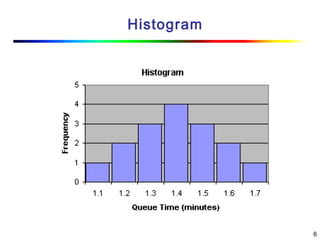
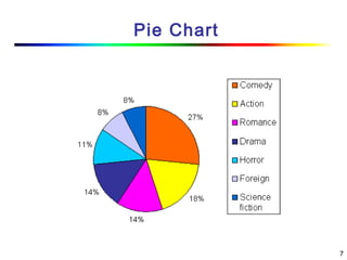

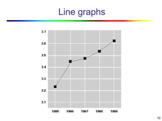


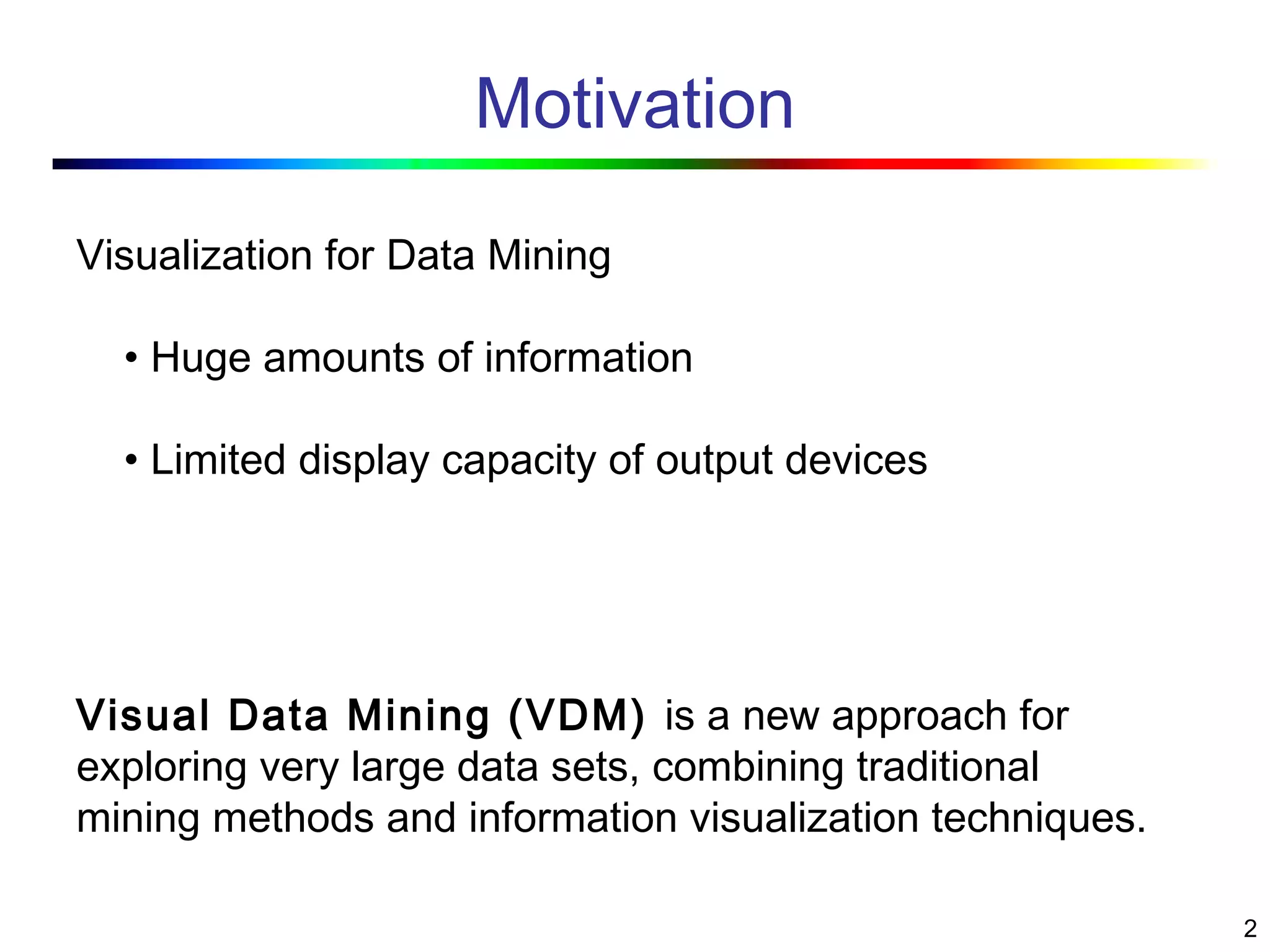
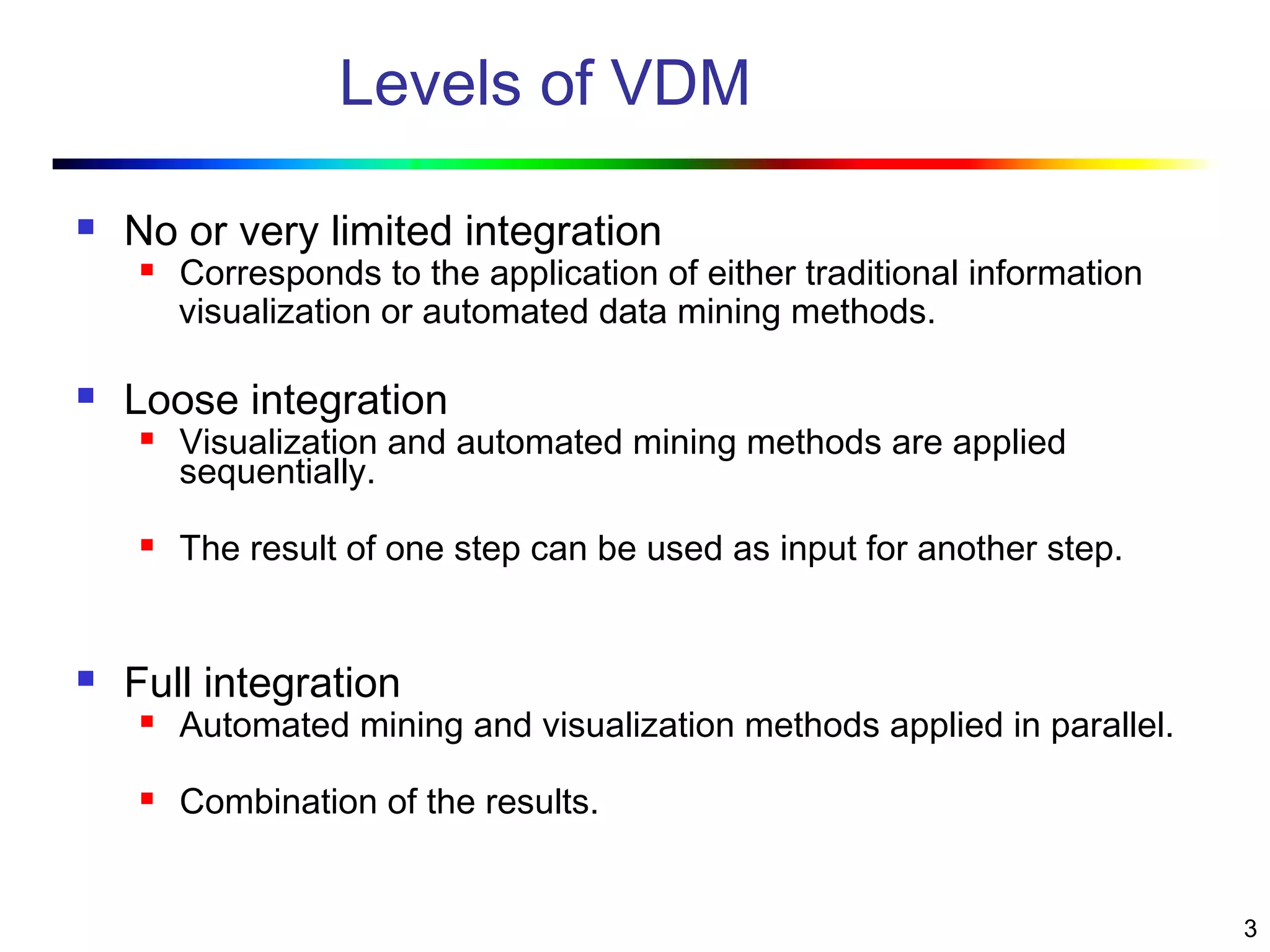

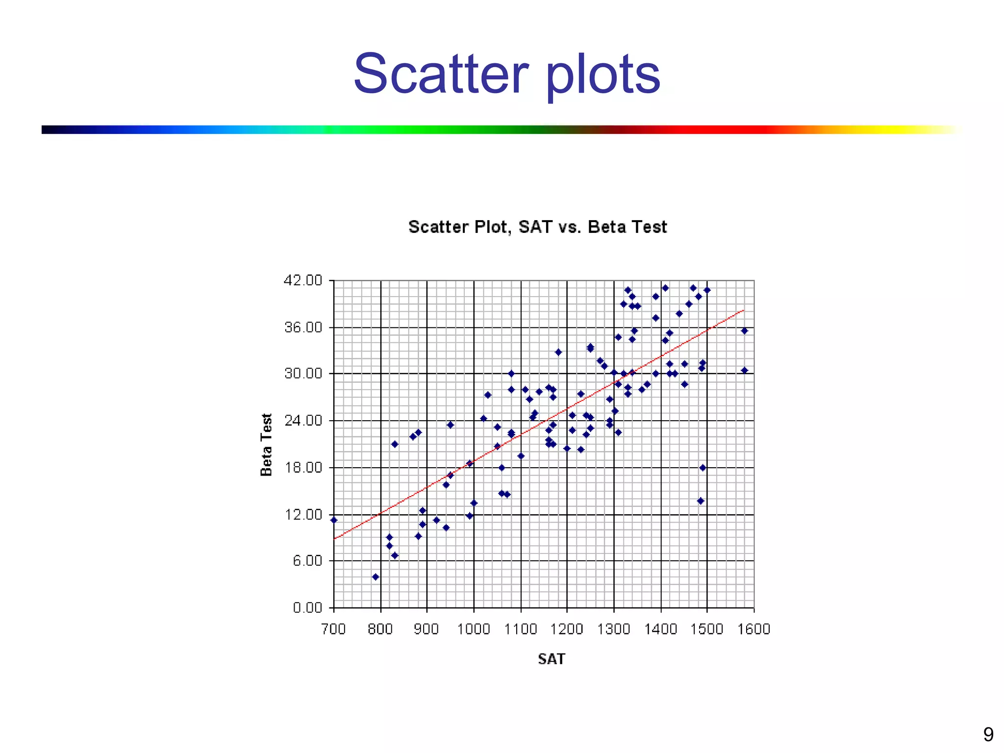
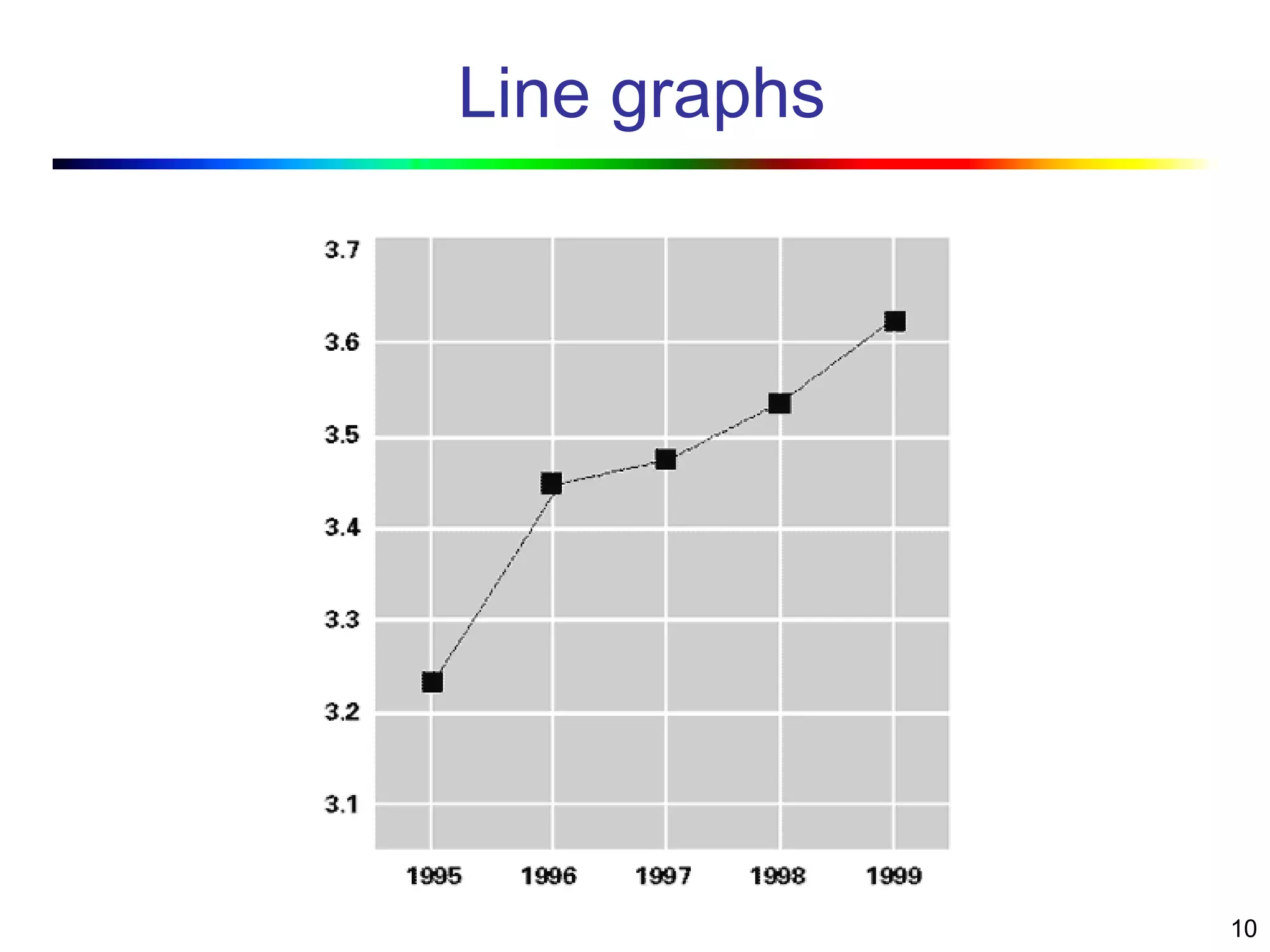
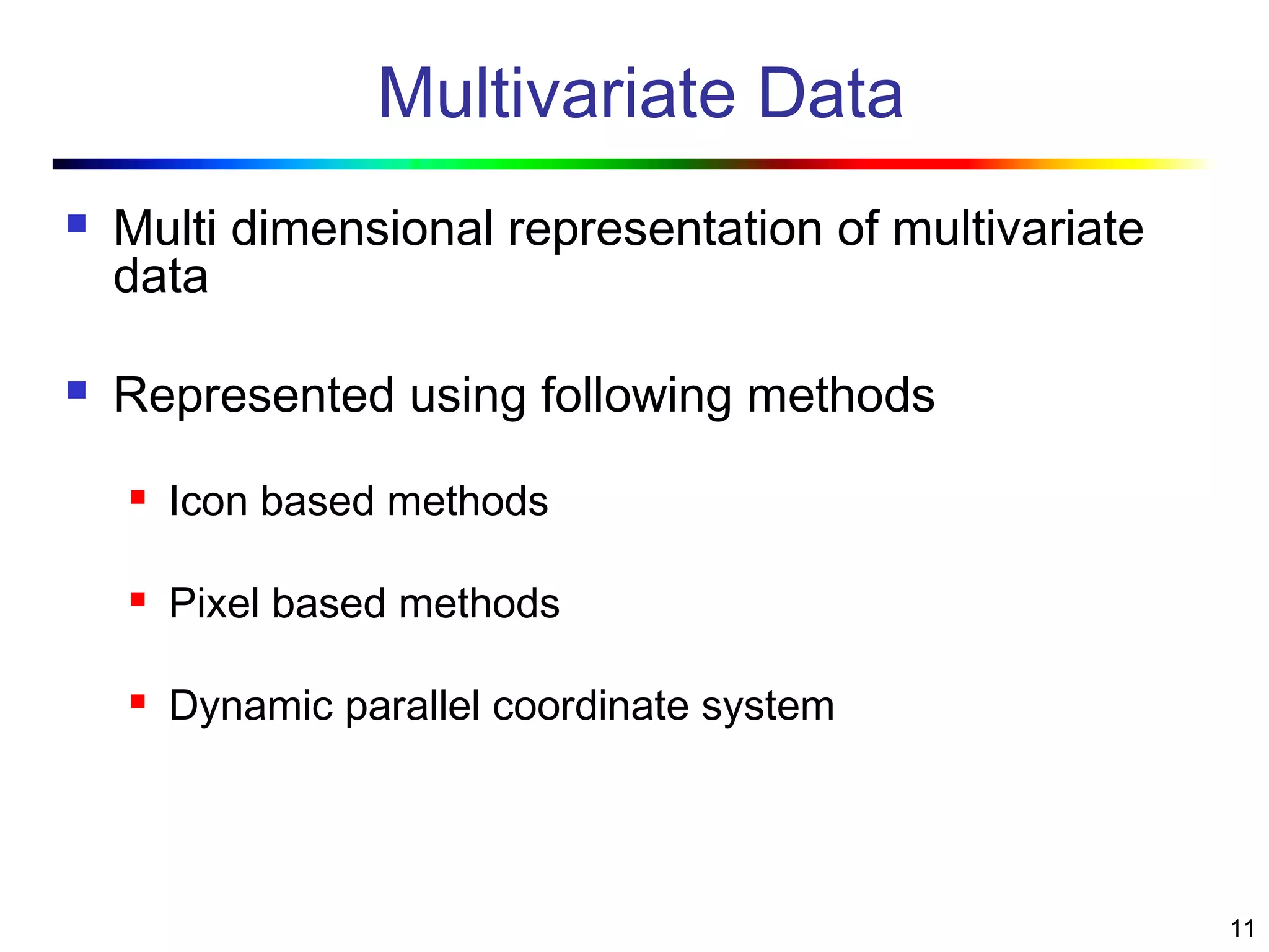

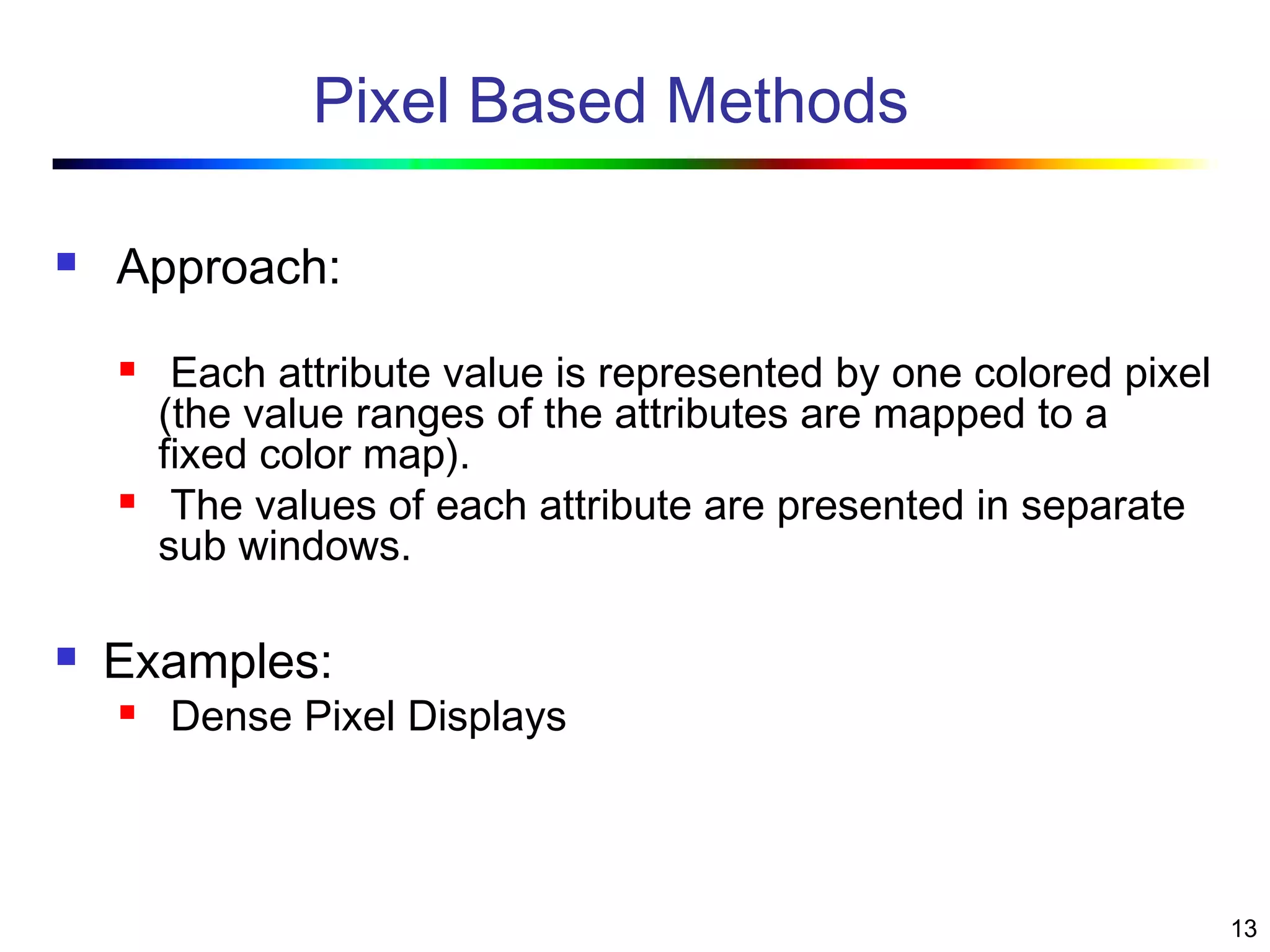
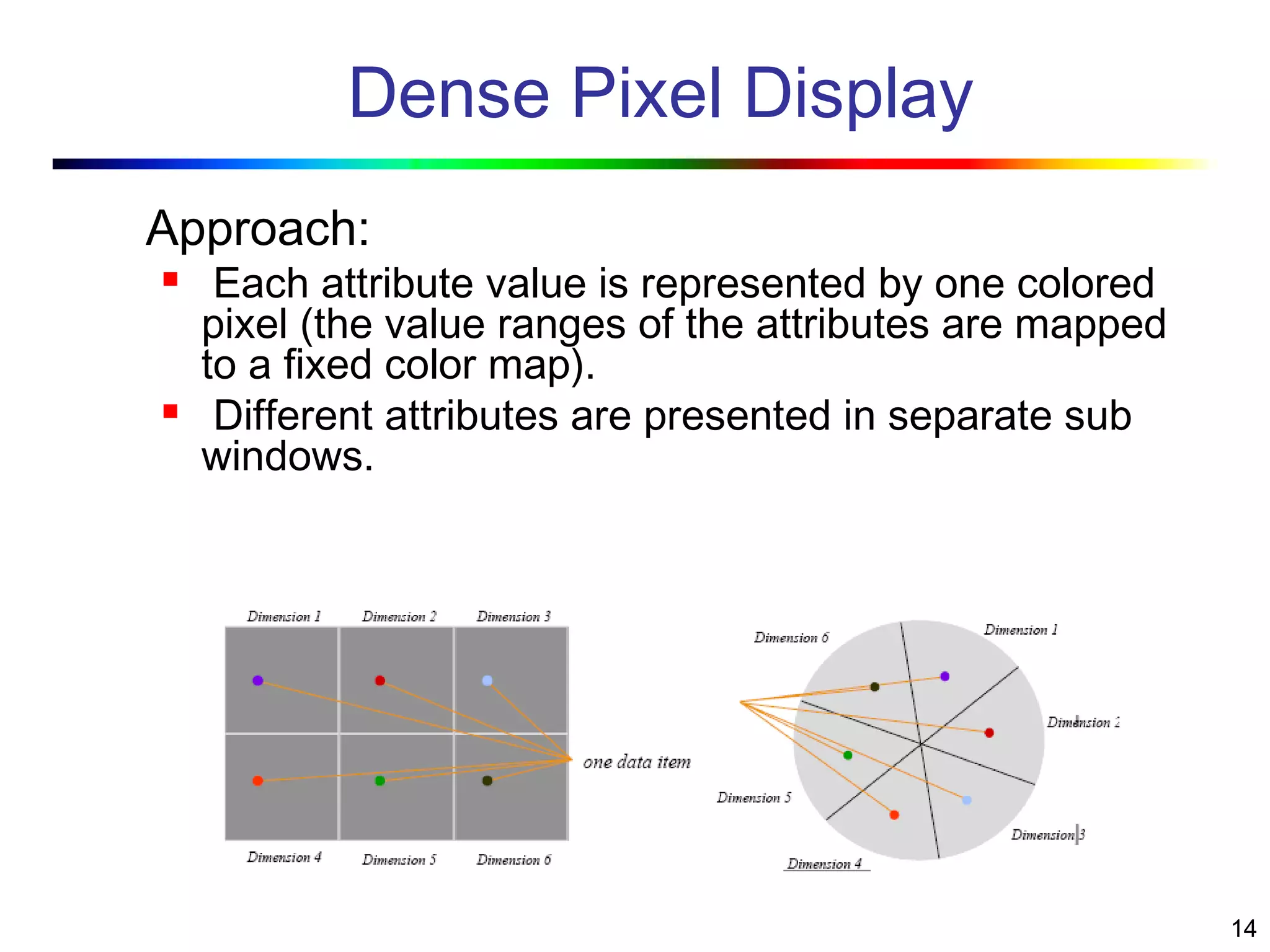

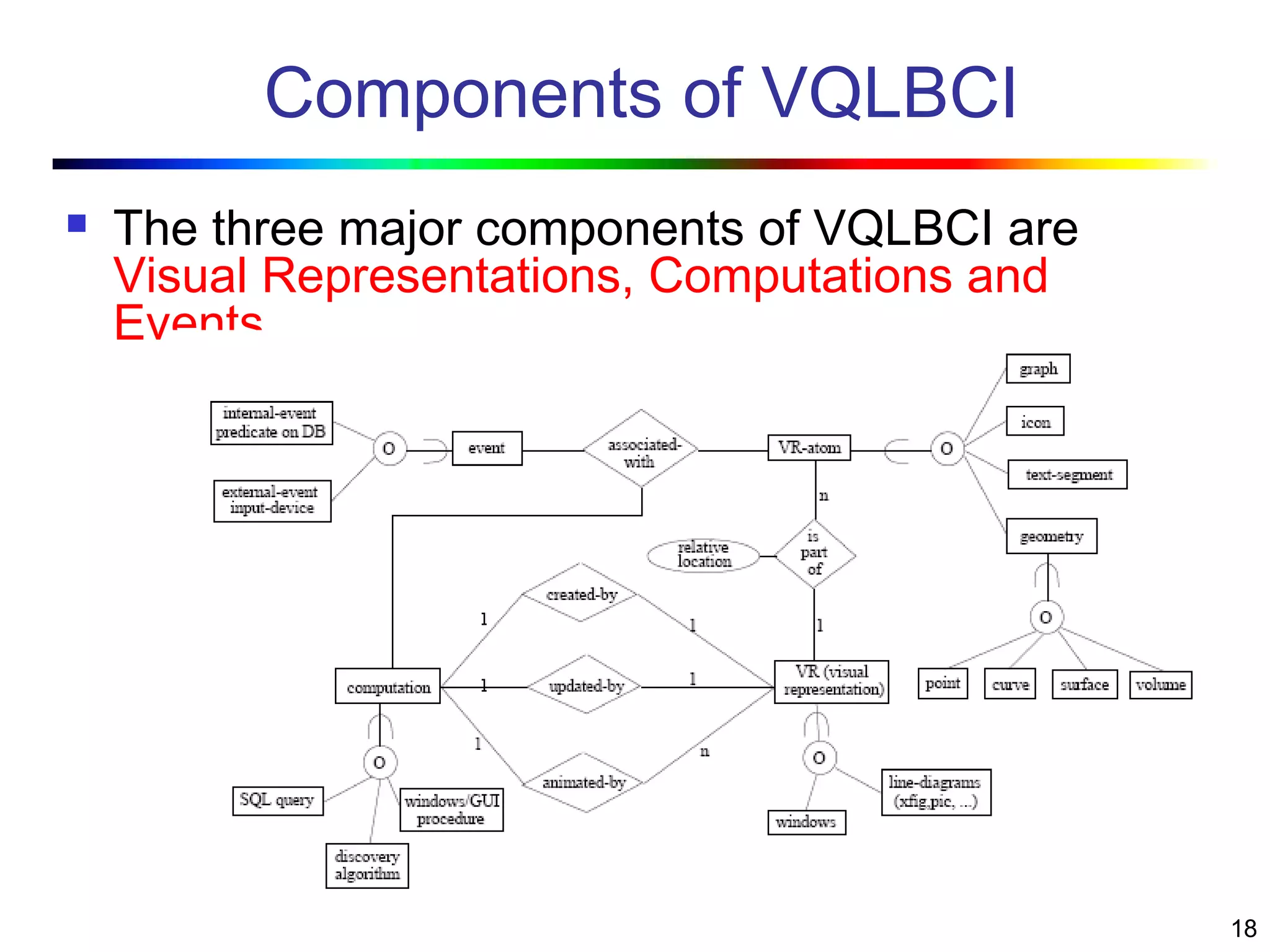


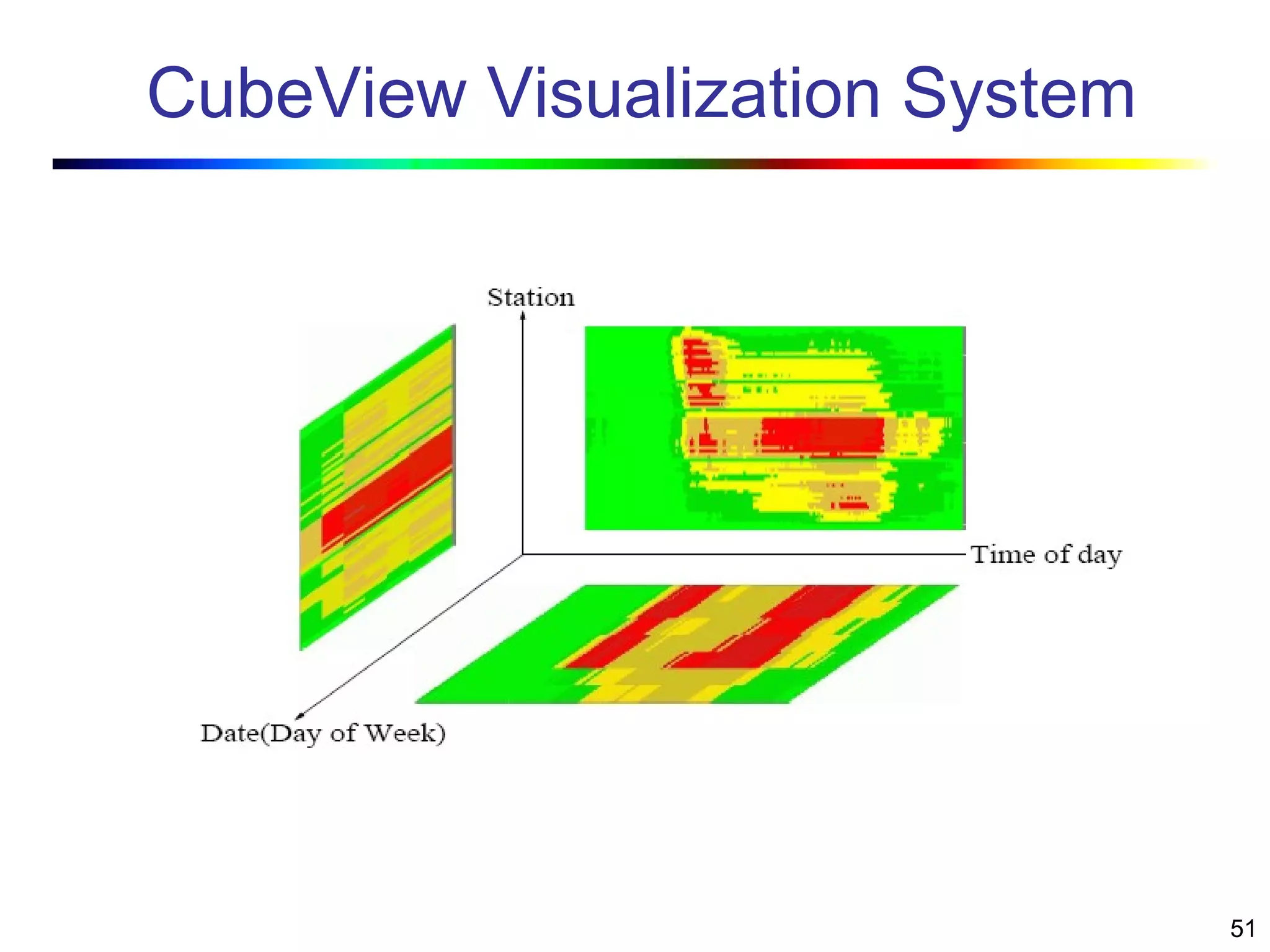
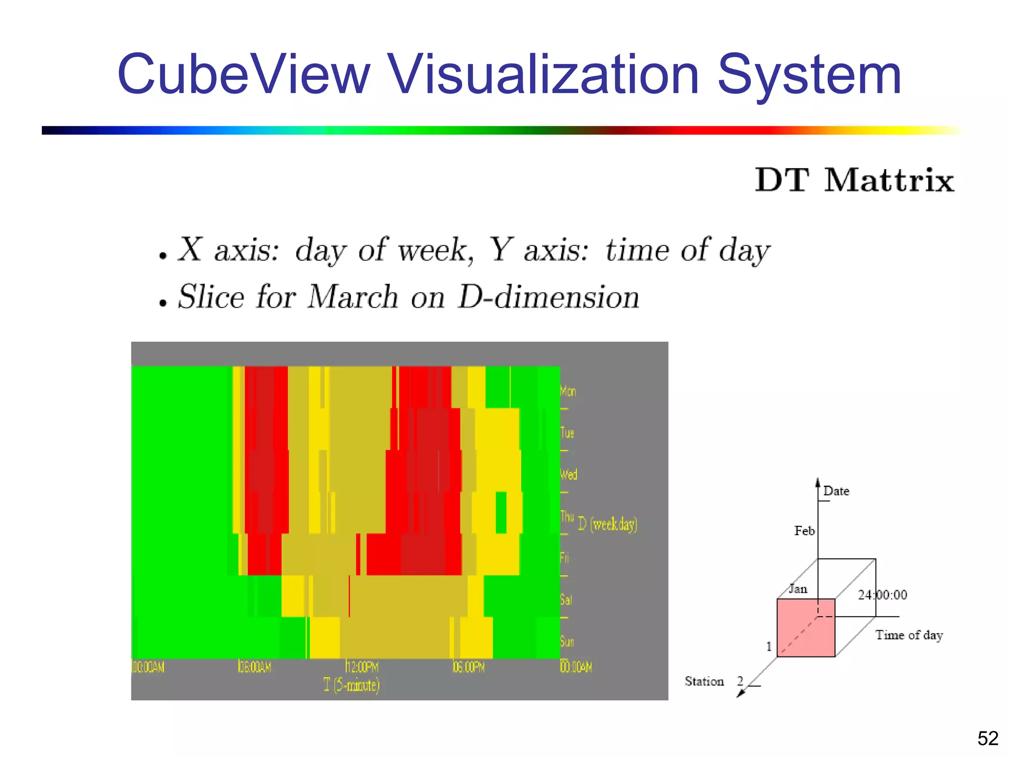
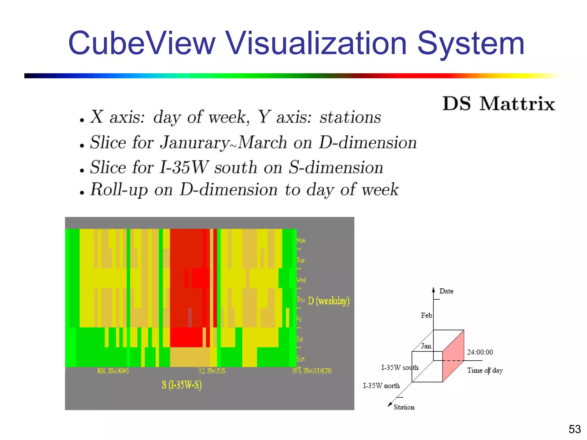
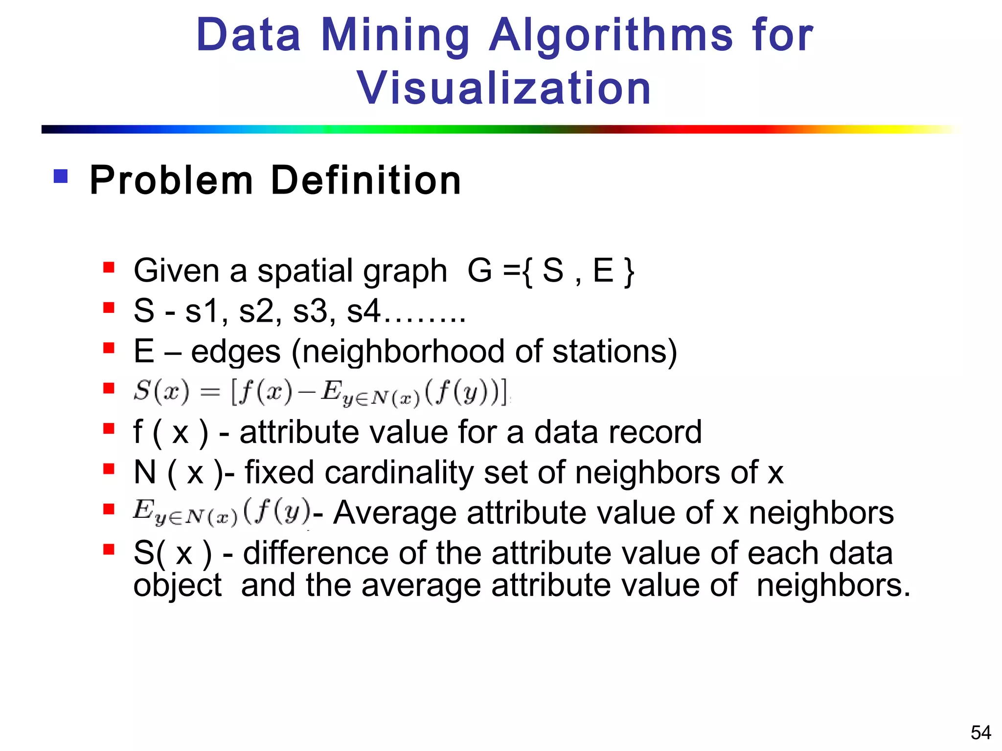


Visual data mining combines traditional data mining methods with information visualization techniques to explore large datasets. There are three levels of integration between visualization and automated mining methods - no/limited integration, loose integration where methods are applied sequentially, and full integration where methods are applied in parallel. Different visualization methods exist for univariate, bivariate and multivariate data based on the type and dimensions of the data. The document describes frameworks and algorithms for visual data mining, including developing new algorithms interactively through a visual interface. It also summarizes a document on using data mining and visualization techniques for selective visualization of large spatial datasets.


