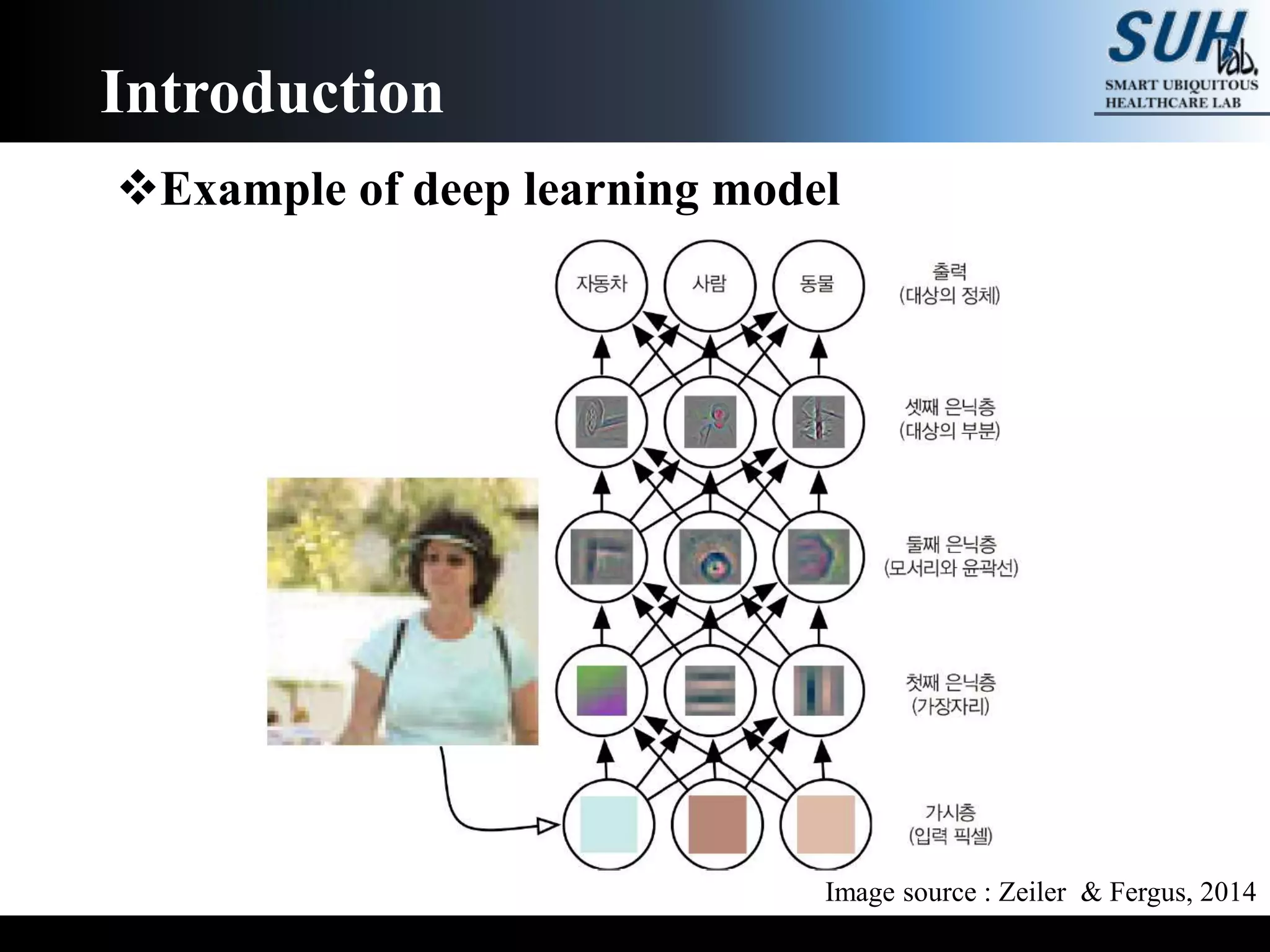
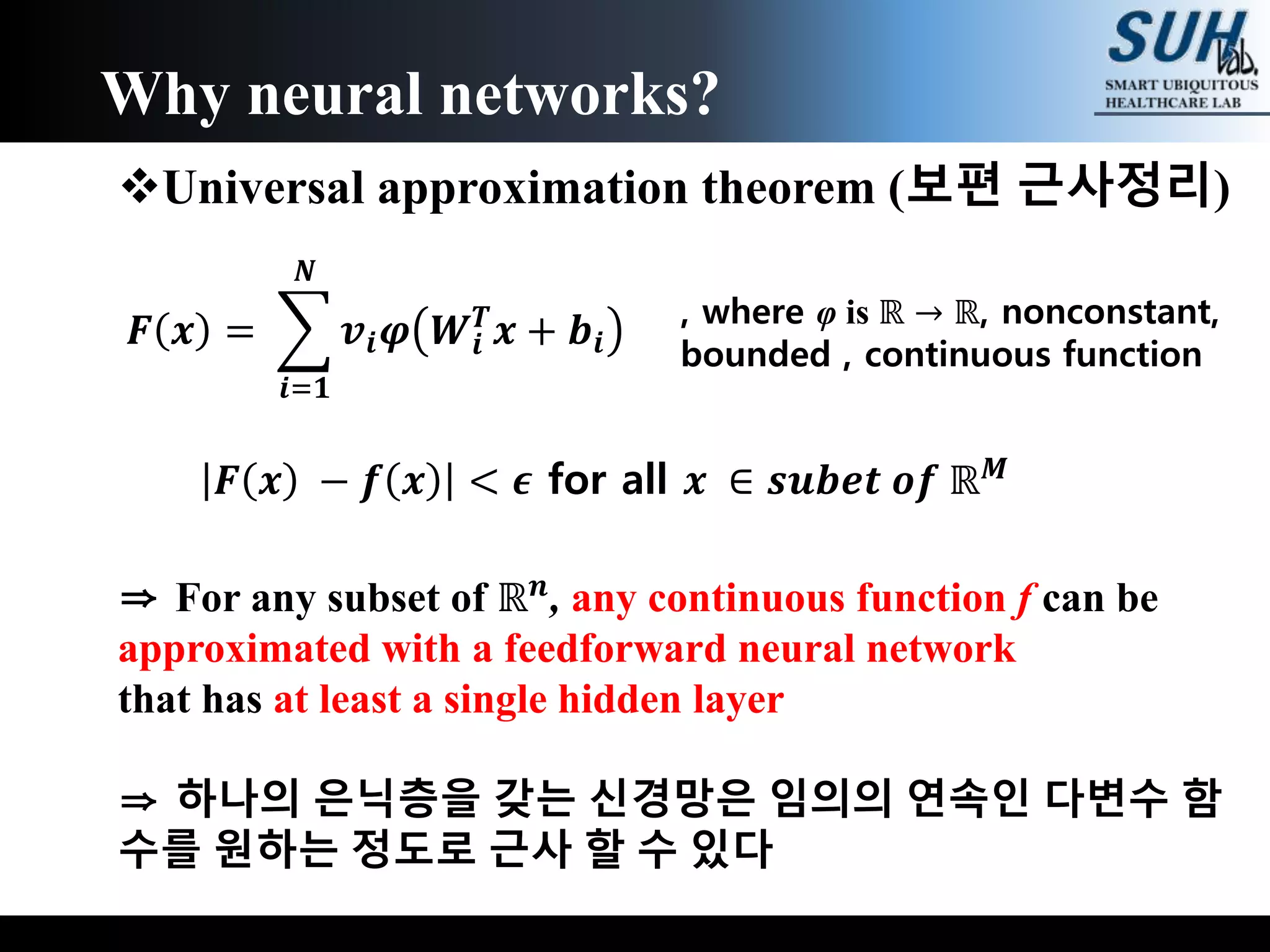
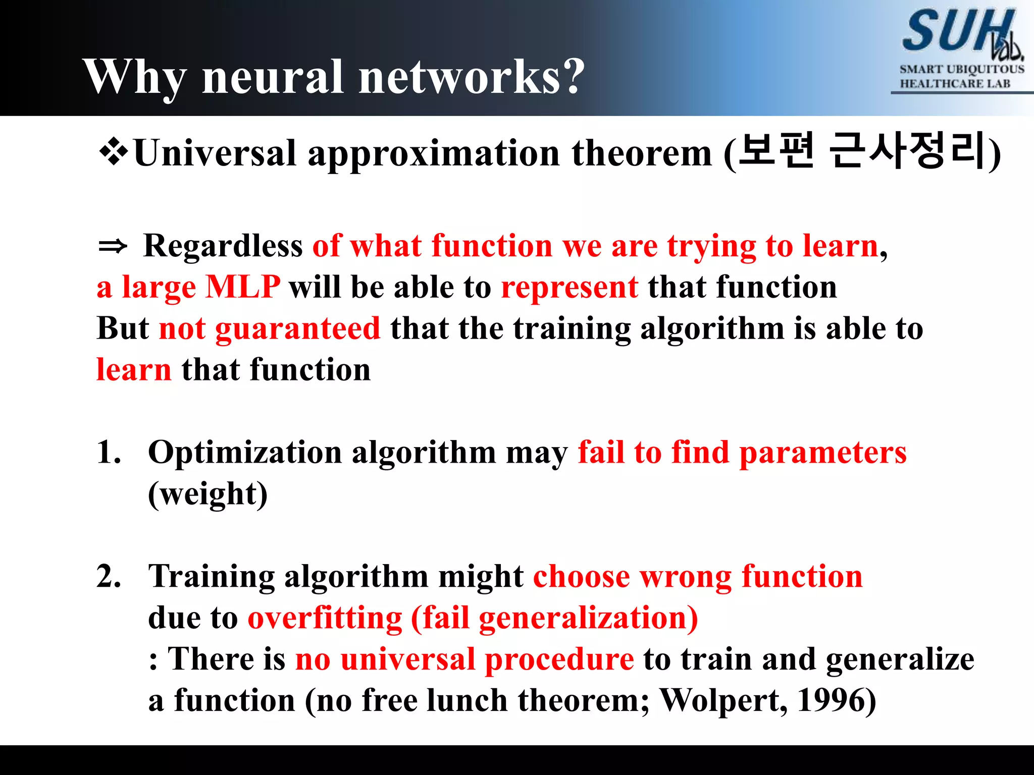
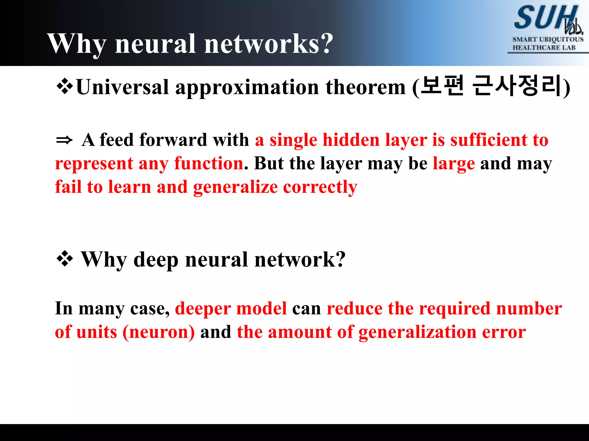
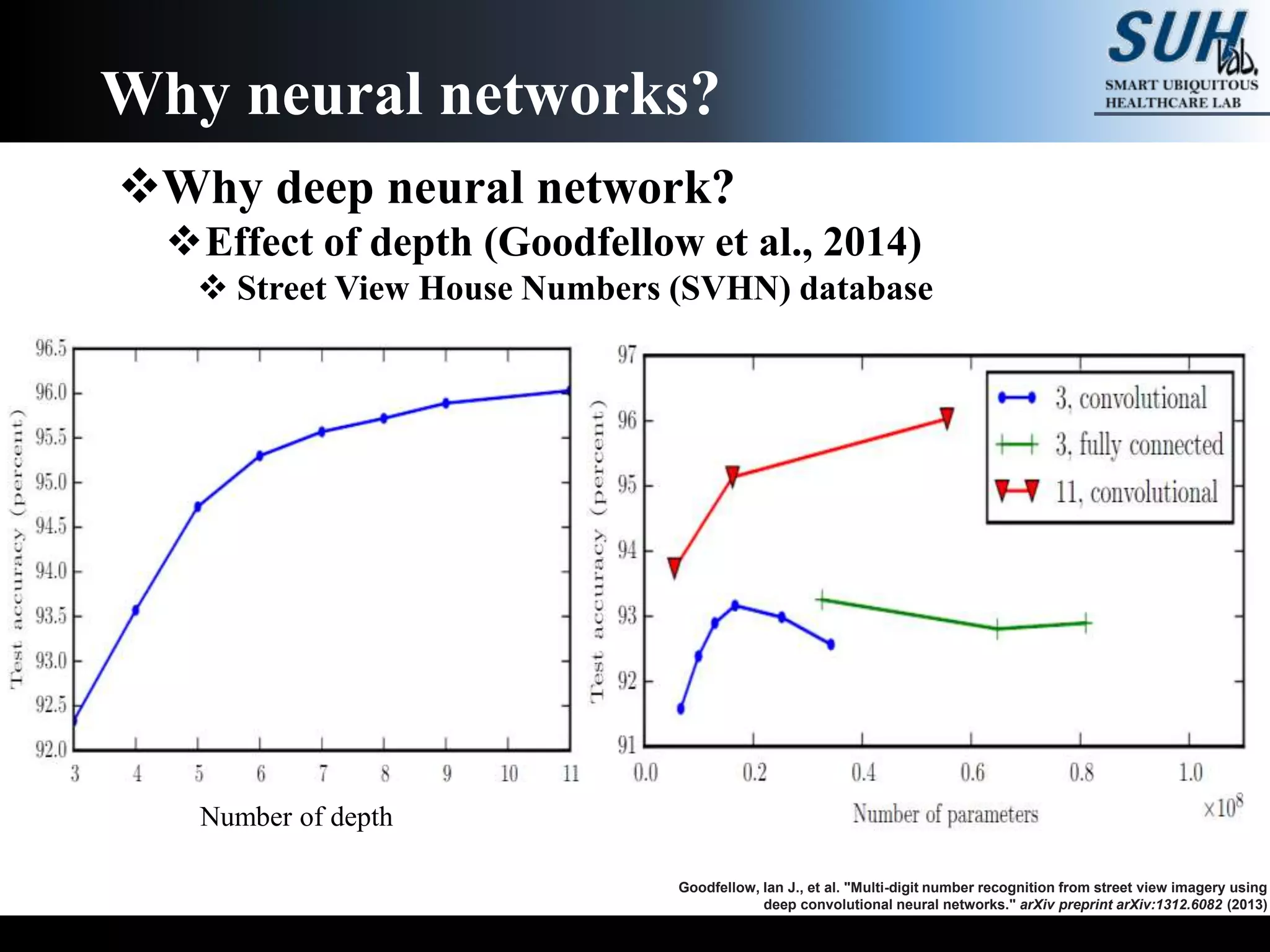
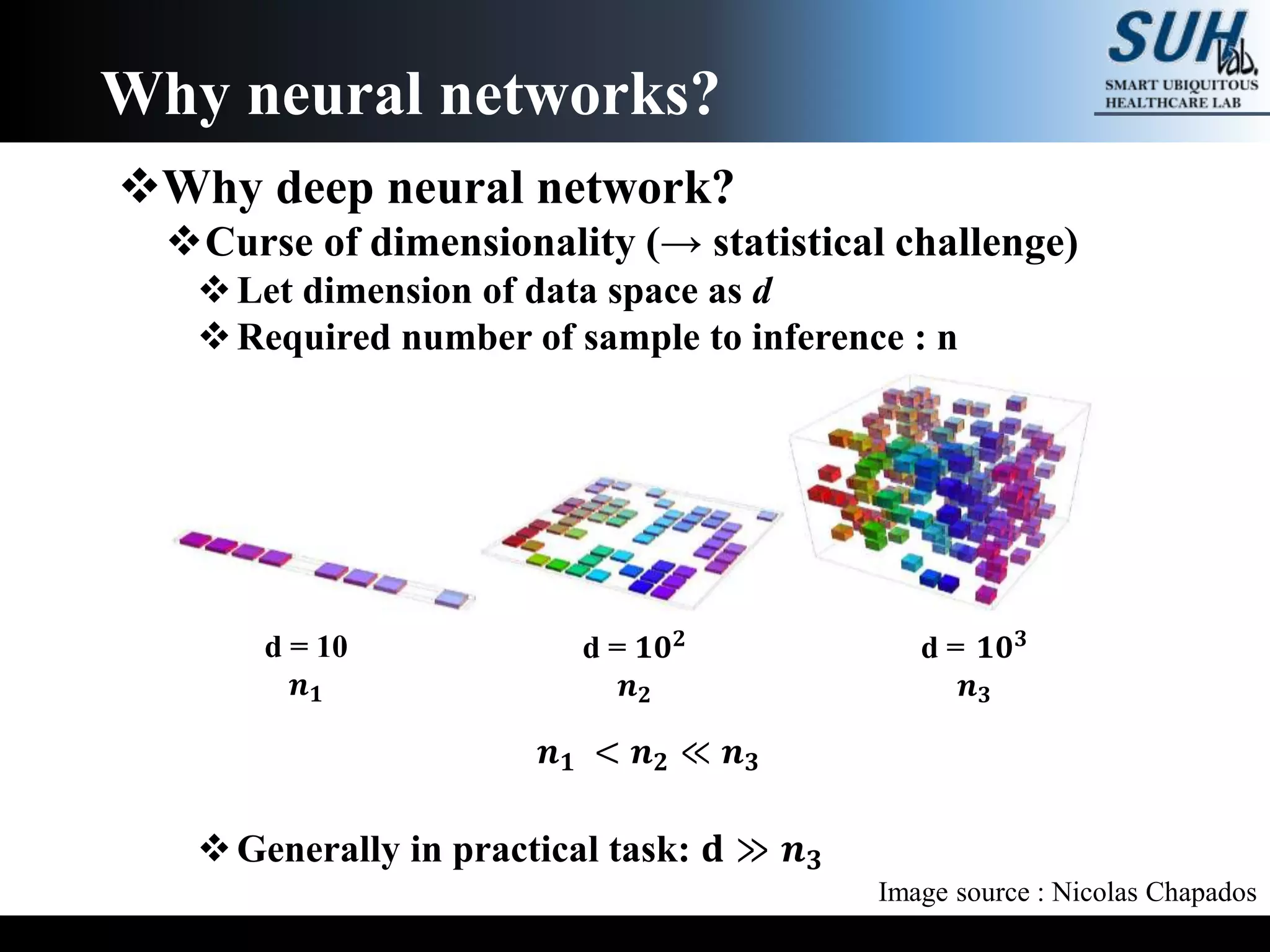
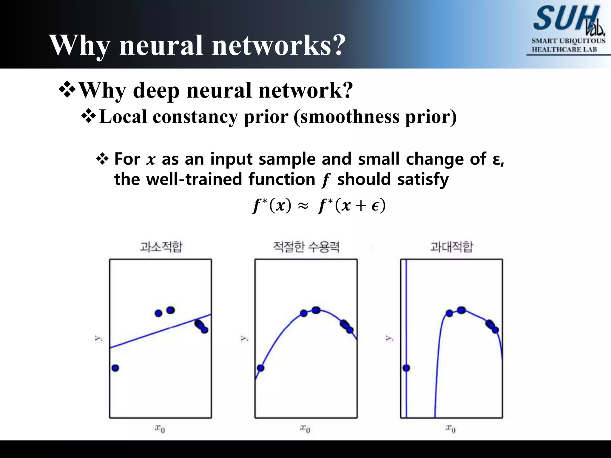
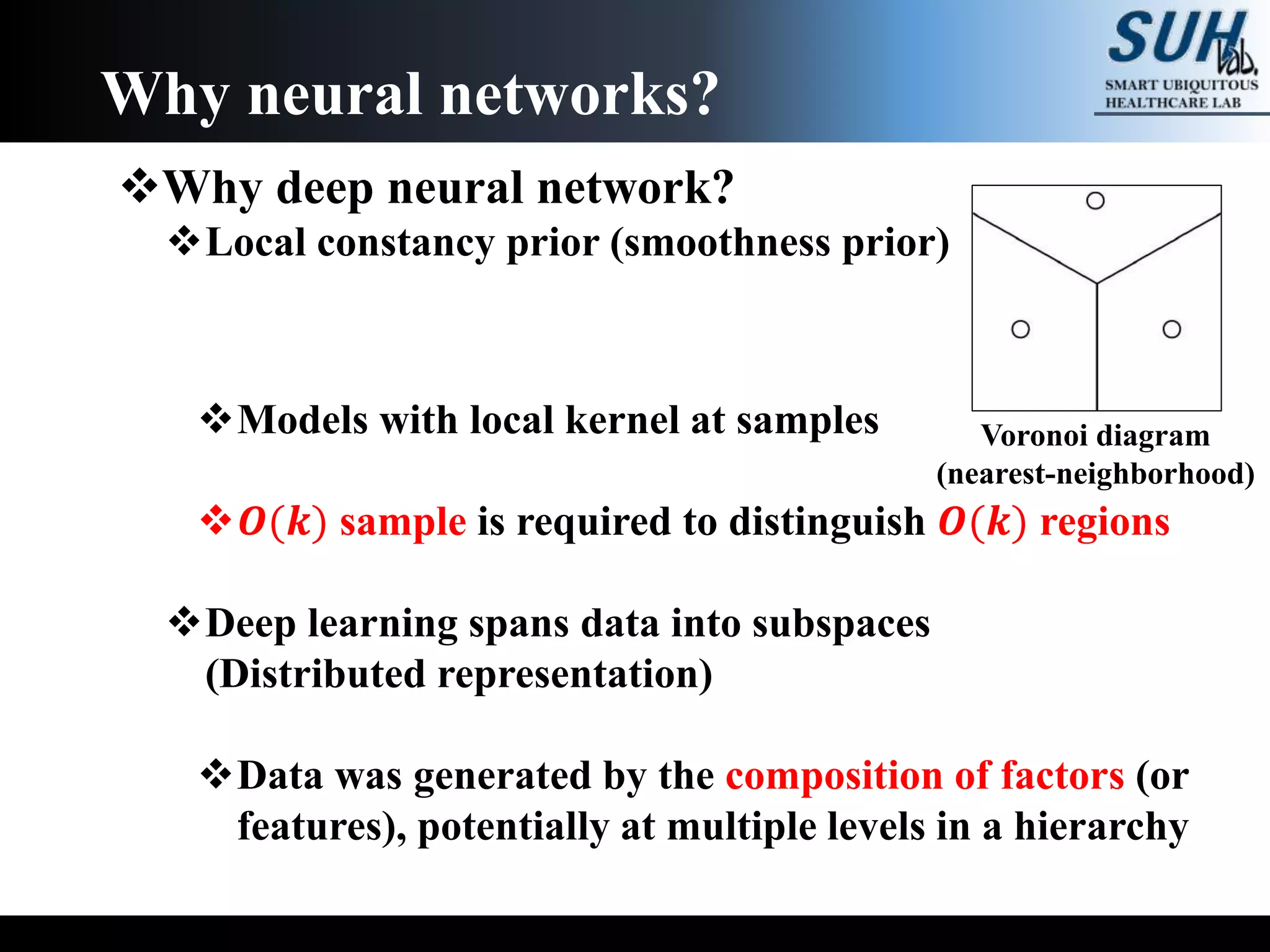
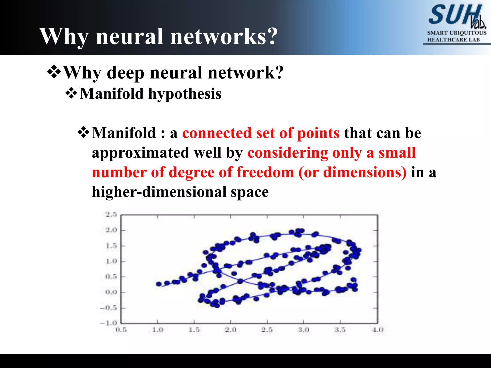
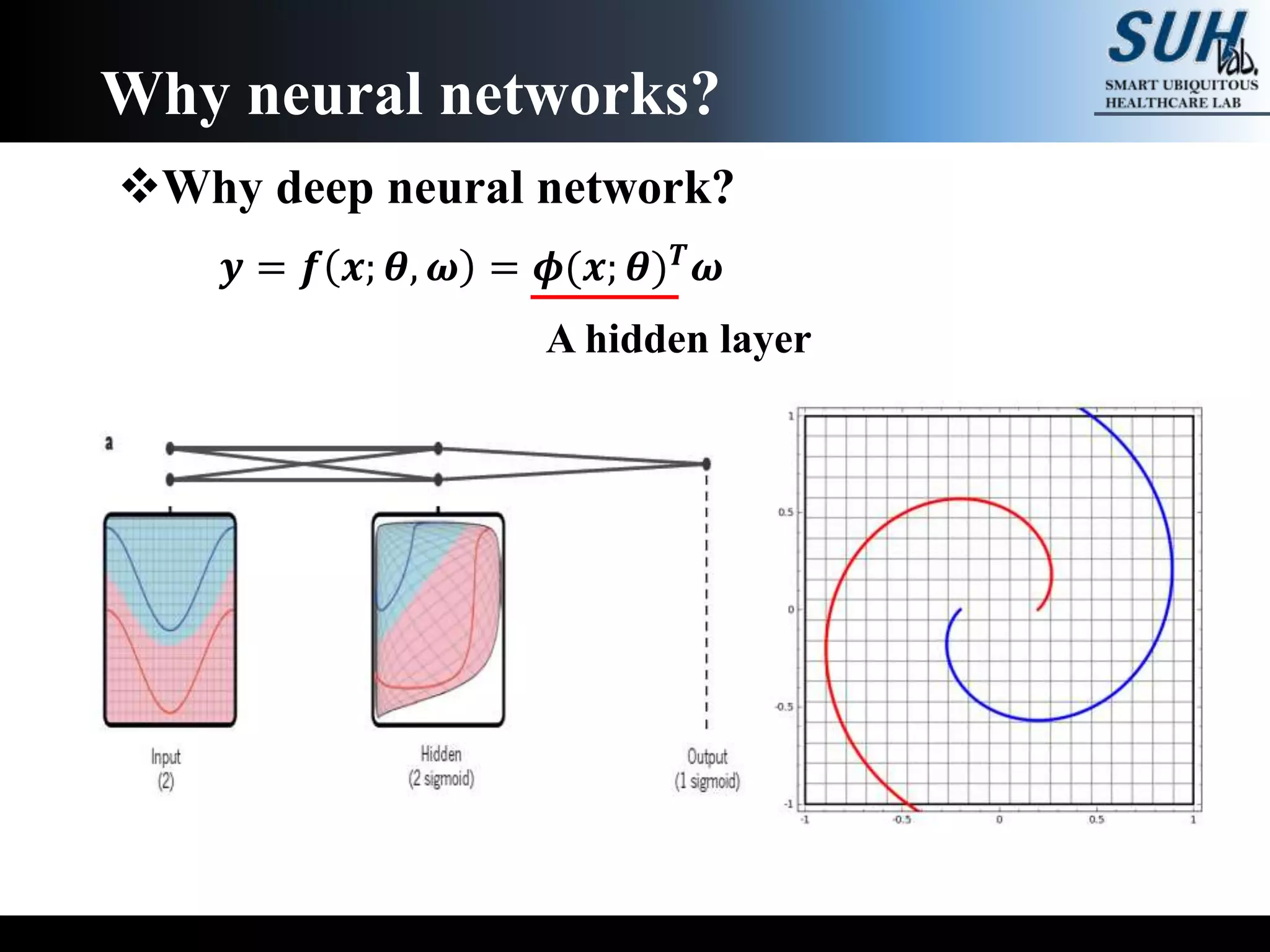
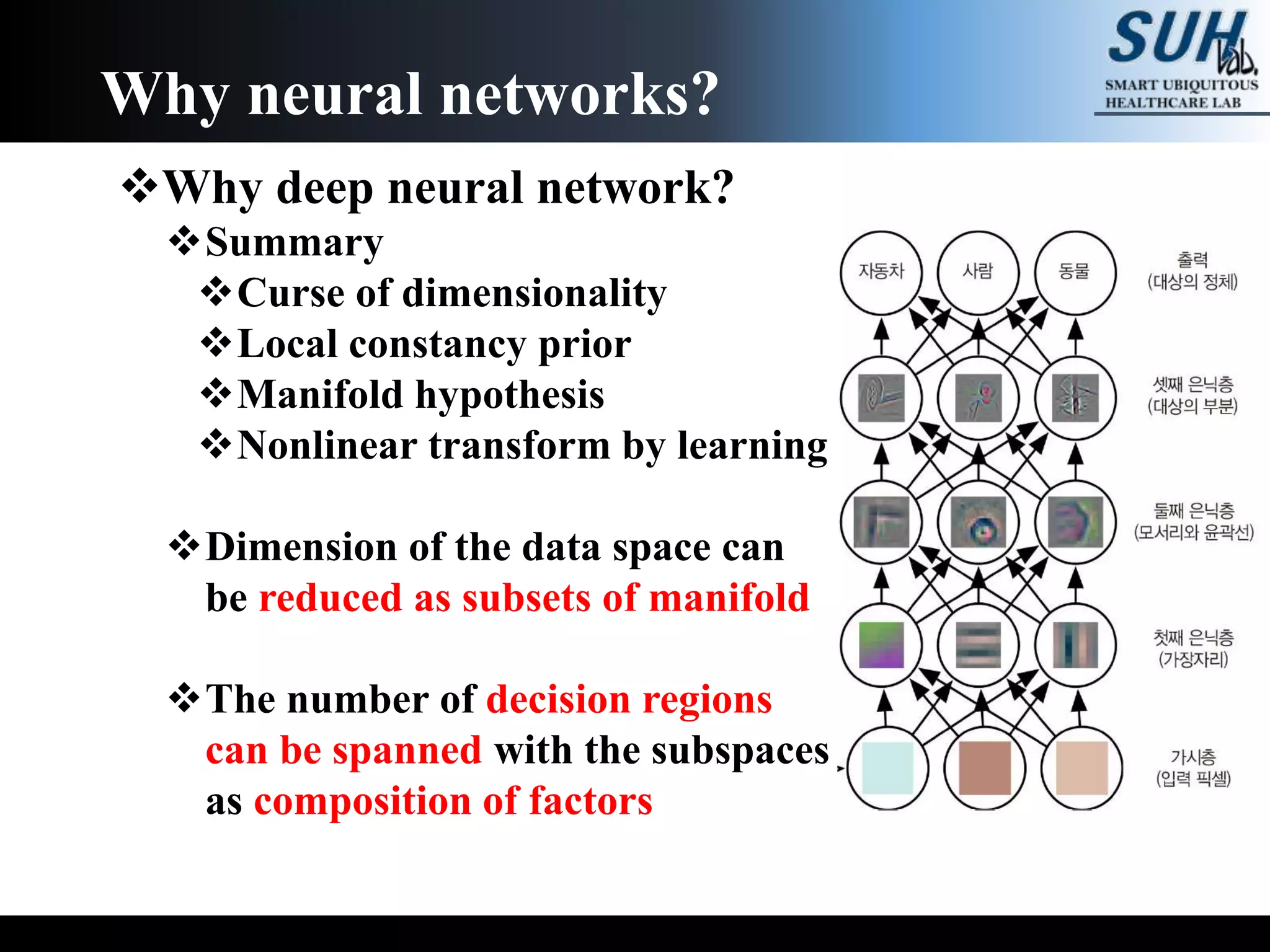
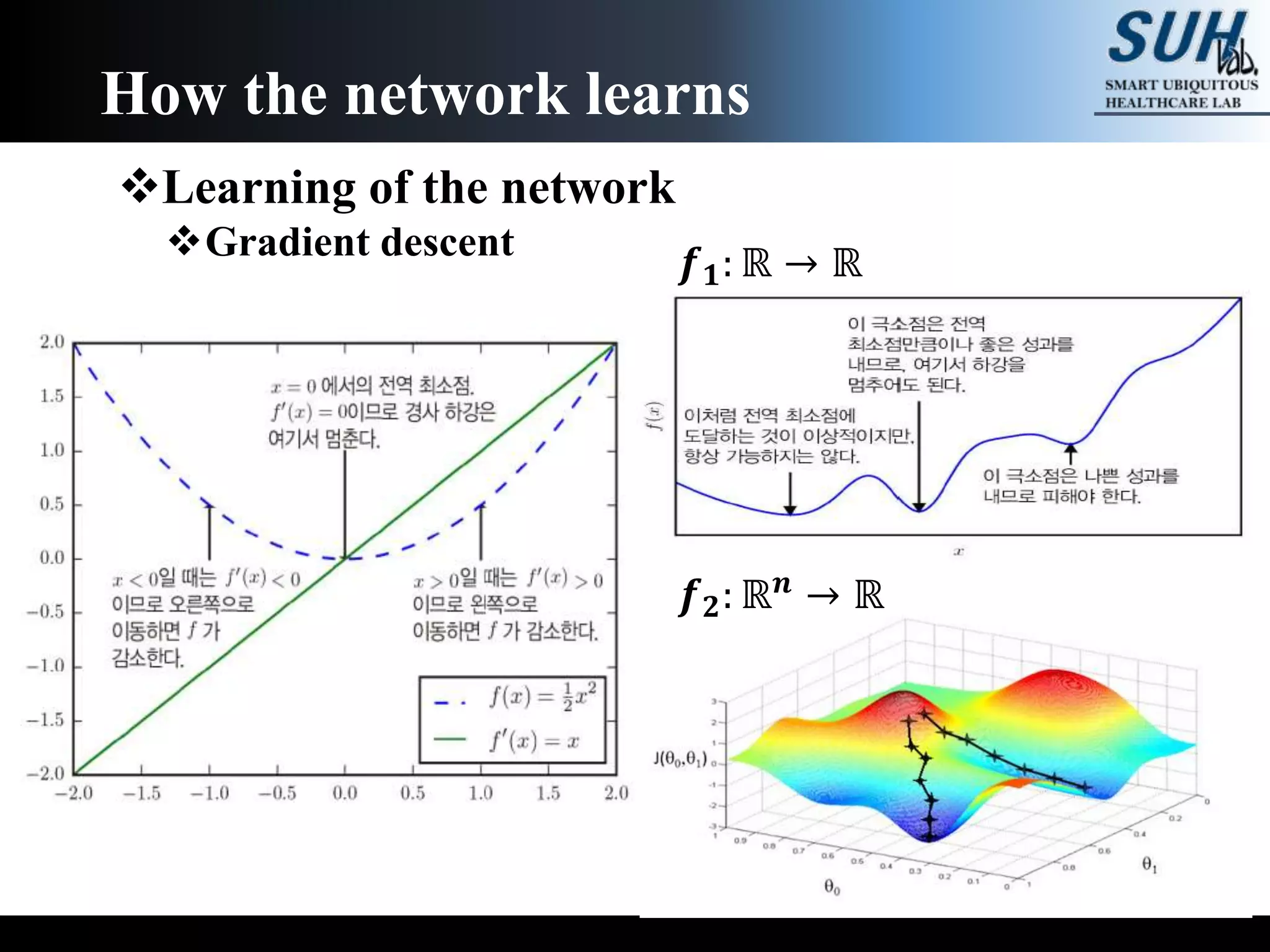
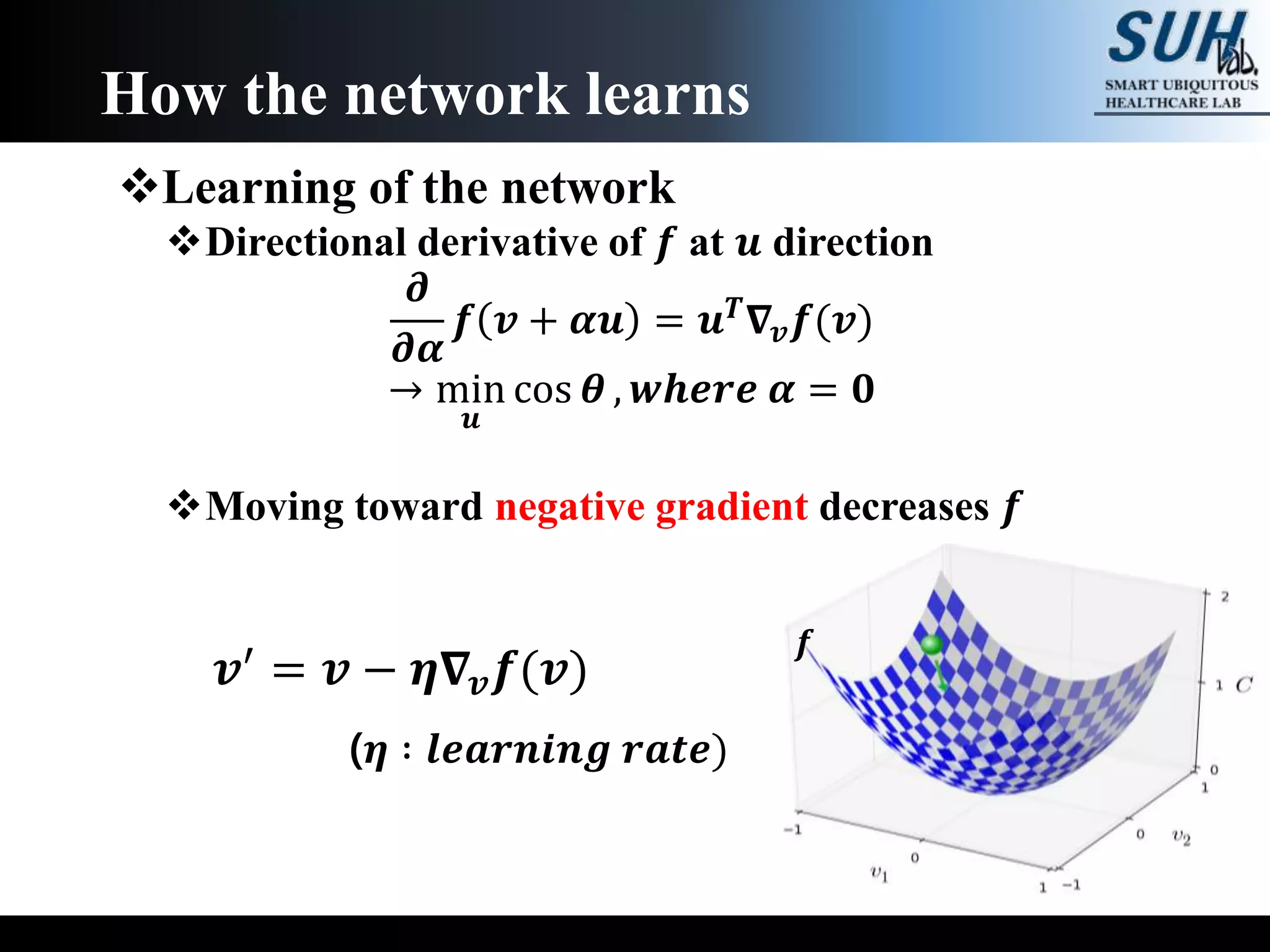
KEMBAR78
Deep learning lecture - part 1 (basics, CNN) | PPTX
Deep Learning
Lecture (1)
19.10.22 You Sung Min
Bengio, Yoshua, Ian Goodfellow, and Aaron
Courville. Deep learning. Vol. 1. MIT press, 2017.
0. Introduction
1. Why neural networks?
1. What is the neural network?
2. Universal approximation theorem
3. Why deep neural network?
2. How the network learns
1. Gradient descent
2. Backpropagation
3. Modern deep learning
1. Convolutional neural network
2. Recurrent neural network
Contents
Example of deep learning model
Introduction
Image source : Zeiler & Fergus, 2014
Artificial intelligence
Introduction
History of deep learning
Introduction
Backpropagation
Distributed representation
(1986)
Deep
learning
(2006)
LSTM
(1997)Biological
learning
(1943)
Neocognitron
(1980)
Perceptron
(1958) Stochastic
gradient descent
(1960)
History of deep learning
 Size of dataset
Introduction
History of deep learning
 Connections per neuron
Introduction
10: GoogleNet
(2014)
History of deep learning
 Number of neurons
Introduction
1. Perceptron
20. GoogleNet
Structure of perceptron (Developed in 1950s)
Why neural networks?
=
𝟎 𝒊𝒇
𝒋
𝝎𝒋 𝒙𝒋 ≤ 𝑻
𝟏 𝒊𝒇
𝒋
𝝎𝒋 𝒙𝒋 > 𝑻
𝝎 𝟏
𝝎 𝟐
𝝎 𝟑
𝒋
𝝎𝒋 𝒙𝒋Binary Inputs
Threshold T
𝒋
𝝎𝒋 𝒙𝒋 − 𝑻 ≤ 𝟎
or
𝒋
𝝎𝒋 𝒙𝒋 − 𝑻 > 𝟎
𝒛 =
𝒋
𝝎𝒋 𝒙𝒋 + 𝒃 𝒐𝒖𝒕𝒑𝒖𝒕 𝒚 = 𝝓(𝒛), where
𝝓 is called activation ftn.
output of a single neuron 𝒚 = 𝝓( 𝒋 𝝎𝒋 𝒙𝒋 + 𝒃)
Multilayer perceptron (MLP)
Why neural networks?
𝝎 𝟏
𝟏
𝝎𝒊
𝒋
𝒚 𝟏
𝟐
𝒙 𝟏
𝒙 𝟐
𝒙𝒊
𝒚𝒋
𝟏
𝒚 𝟐
𝟏
𝒚 𝟏
𝟏
𝒚𝒋
𝟏
= 𝝓(
𝒊
𝝎𝒊
𝟏
𝒙𝒊 + 𝒃𝒋
𝟏
)
𝒚 𝟏
𝟐
= 𝝓(
𝒊
𝝎𝒊
𝟐
𝒚𝒊
𝟏
+ 𝒃𝒋
𝟐
)
𝒚 𝟑
𝝎 𝟏
𝟐
𝝎 𝟏
𝟑
𝒚 𝟑 = 𝝓(
𝒊
𝝎𝒊
𝟑
𝒚𝒊
𝟐
+ 𝒃𝒋
𝟑
)
𝑭 𝒙 = 𝝓
𝒊
𝝎𝒊
𝟑
𝝓(
𝒊
𝝎𝒊
𝟐
𝝓(
𝒊
𝝎𝒊
𝟏
𝒙𝒊 + 𝒃𝒋
𝟏
) + 𝒃𝒋
𝟐
) + 𝒃𝒋
𝟑
Output of a network
Universal approximation theorem (보편 근사정리)
⇒ For any subset of ℝ 𝒏, any continuous function f can be
approximated with a feedforward neural network
that has at least a single hidden layer
⇒ 하나의 은닉층을 갖는 신경망은 임의의 연속인 다변수 함
수를 원하는 정도로 근사 할 수 있다
Why neural networks?
𝑭 𝒙 =
𝒊=𝟏
𝑵
𝒗𝒊 𝝋 𝑾𝒊
𝑻
𝒙 + 𝒃𝒊
, where φ is ℝ → ℝ, nonconstant,
bounded , continuous function
𝑭 𝒙 − 𝒇 𝒙 < 𝝐 for all 𝒙 ∈ 𝒔𝒖𝒃𝒆𝒕 𝒐𝒇 ℝ 𝑴
Universal approximation theorem (보편 근사정리)
⇒ Regardless of what function we are trying to learn,
a large MLP will be able to represent that function
But not guaranteed that the training algorithm is able to
learn that function
1. Optimization algorithm may fail to find parameters
(weight)
2. Training algorithm might choose wrong function
due to overfitting (fail generalization)
: There is no universal procedure to train and generalize
a function (no free lunch theorem; Wolpert, 1996)
Why neural networks?
Universal approximation theorem (보편 근사정리)
⇒ A feed forward with a single hidden layer is sufficient to
represent any function. But the layer may be large and may
fail to learn and generalize correctly
 Why deep neural network?
In many case, deeper model can reduce the required number
of units (neuron) and the amount of generalization error
Why neural networks?
Why deep neural network?
Effect of depth (Goodfellow et al., 2014)
 Street View House Numbers (SVHN) database
Why neural networks?
Number of depth
Goodfellow, Ian J., et al. "Multi-digit number recognition from street view imagery using
deep convolutional neural networks." arXiv preprint arXiv:1312.6082 (2013)
Why deep neural network?
Curse of dimensionality (→ statistical challenge)
Let dimension of data space as d
Required number of sample to inference : n
Generally in practical task: 𝐝 ≫ 𝒏 𝟑
Why neural networks?
Image source : Nicolas Chapados
d = 10
𝒏 𝟏
d = 𝟏𝟎 𝟐
𝒏 𝟐
d = 𝟏𝟎 𝟑
𝒏 𝟑
𝒏 𝟏 < 𝒏 𝟐 ≪ 𝒏 𝟑
Why deep neural network?
Local constancy prior (smoothness prior)
 For 𝒙 as an input sample and small change of ε,
the well-trained function 𝒇 should satisfy
Why neural networks?
𝒇∗
𝒙 ≈ 𝒇∗
𝒙 + 𝝐
Why deep neural network?
Local constancy prior (smoothness prior)
Models with local kernel at samples
𝑶(𝒌) sample is required to distinguish 𝑶(𝒌) regions
Deep learning spans data into subspaces
(Distributed representation)
Data was generated by the composition of factors (or
features), potentially at multiple levels in a hierarchy
Why neural networks?
Voronoi diagram
(nearest-neighborhood)
Why deep neural network?
Manifold hypothesis
Manifold : a connected set of points that can be
approximated well by considering only a small
number of degree of freedom (or dimensions) in a
higher-dimensional space
Why neural networks?
Why deep neural network?
Manifold hypothesis
Real world data(sound, image, text etc.) are highly
concentrated
Why neural networks?
Random samples in the image space
Why deep neural network?
Manifold hypothesis
Even though the data space is ℝ 𝒏, we don’t have to
consider all the space
We may consider only neighborhood of the observed
samples along with some manifolds
A transfer may exist along the manifold
For example, intensity change in images
 Manifolds related human face and those related with cat
may different
Why neural networks?
Why deep neural network?
Manifold hypothesis
Why neural networks?
Radford, Alec, Luke Metz, and Soumith Chintala. "Unsupervised representation learning with
deep convolutional generative adversarial networks." arXiv preprint arXiv:1511.06434 (2015)
Why deep neural network?
 Non-linear transform by learning
Linear model: linear combination of input 𝑿
⇒ Linear model with non-linear transform 𝝓(𝑿) as
input
Finding an optimal 𝝓 𝑿
Previous: human knowledge-based transform
(i.e., handcrafted features)
Deep learning: learning inside the network
𝒚 = 𝒇 𝒙; 𝜽, 𝝎 = 𝝓(𝒙; 𝜽) 𝑻 𝝎
Why neural networks?
Why deep neural network?
Why neural networks?
A hidden layer
𝒚 = 𝒇 𝒙; 𝜽, 𝝎 = 𝝓(𝒙; 𝜽) 𝑻 𝝎
Why deep neural network?
Summary
Curse of dimensionality
Local constancy prior
Manifold hypothesis
Nonlinear transform by learning
Dimension of the data space can
be reduced as subsets of manifold
The number of decision regions
can be spanned with the subspaces
as composition of factors
Why neural networks?
Learning of the network
To approximate a function 𝒇∗
Classifier 𝒚 = 𝒇∗(𝒙), where 𝒚𝒊 ∈ 𝒇𝒊𝒏𝒊𝒕𝒆 𝒔𝒆𝒕
Regression 𝒚 = 𝒇∗
(𝒙), where 𝒚𝒊 ∈ ℝ 𝒅
 A network defines a mapping 𝒚 = 𝒇(𝒙; 𝜽) and
learns parameters 𝜽 which approximate the function 𝒇∗
Due to the non-linearity, the global optimization
algorithm (such as convex optimization) is not proper to
the deep learning → Update cost function 𝑪
Gradient descent
Backpropagation
How the network learns
Learning of the network
Gradient descent
How the network learns
𝒇 𝟏: ℝ → ℝ
𝒇 𝟐: ℝ 𝒏 → ℝ
Learning of the network
Directional derivative of 𝒇 at 𝒖 direction
𝝏
𝝏𝜶
𝒇 𝒗 + 𝜶𝒖 = 𝒖 𝑻 𝛁𝒗 𝒇(𝒗)
→ min
𝒖
cos 𝜽 , 𝒘𝒉𝒆𝒓𝒆 𝜶 = 𝟎
Moving toward negative gradient decreases 𝒇
How the network learns
𝒇
𝒗′ = 𝒗 − 𝜼𝛁𝒗 𝒇(𝒗)
(𝜼 ∶ 𝒍𝒆𝒂𝒓𝒏𝒊𝒏𝒈 𝒓𝒂𝒕𝒆)
Learning of the network
Backpropagation
How the network learns
Error backpropagation path
𝒙 𝒚 = 𝒈(𝒙)
𝒅𝒛
𝒅𝒙
=
𝒅𝒛
𝒅𝒚
𝒅𝒚
𝒅𝒙
𝒛 = 𝒇 𝒈 𝒙
= 𝒇(𝒚)y
𝒛
by chain-rule
Learning of the network
Backpropagation
For 𝒙 ∈ ℝ 𝒎
, 𝒚 ∈ ℝ 𝒏
and 𝒈: ℝ 𝒎
→ ℝ 𝒏
, 𝒇: ℝ 𝒏
→ ℝ
From gradient descent,
How the network learns
𝒅𝒛
𝒅𝒙
=
𝒅𝒛
𝒅𝒚
𝒅𝒚
𝒅𝒙
𝝏𝒛
𝝏𝒙𝒊
=
𝒋
𝝏𝒛
𝝏𝒚𝒋
𝝏𝒚𝒋
𝝏𝒙𝒊
𝛁𝒙 𝒛 = (
𝝏𝒚
𝝏𝒙
) 𝑻
𝛁𝒚 𝒛
𝝏𝒚
𝝏𝒙
: 𝒏 × 𝒎 Jacobian
matrix of 𝒈
𝒙′ = 𝒙 − 𝜼(
𝝏𝒚
𝝏𝒙
) 𝑻 𝛁𝒚 𝒛 𝜽′ = 𝜽 − 𝜼(
𝝏𝒚
𝝏𝜽
) 𝑻 𝛁𝒚 𝒛
Learning of the network
Universal approximation theorem
Gradient descent & Backpropagation
Practical reason of fail
Optimization
Optimizer (SGD, AdaGrad, RMSprop, Adam, etc.)
Weight initialization
Regularization
Parameter norm penalty (𝑳 𝟐
, 𝑳 𝟏
)
Augmentation / Noise input (weight noise, label smoothing)
Multitask learning
Parameter sharing (CNN)
Ensemble / Dropout
Adversarial training
How the network learns
Domain specific prior
Convolutional neural network
Convolution vs cross-correlation
Convolution
Cross-correlation
Modern deep learning
𝑺 𝒊, 𝒋 = 𝑰 ∗ 𝑲 𝒊, 𝒋 =
𝒎 𝒏
𝑰 𝒎, 𝒏 𝑲(𝒊 − 𝒎, 𝒋 − 𝒏)
= 𝑲 ∗ 𝑰 𝒊, 𝒋 =
𝒎 𝒏
𝑰 𝒊 − 𝒎, 𝒋 − 𝒏 𝑲(𝒎, 𝒏)
𝑺 𝒊, 𝒋 = 𝑰 ∗ 𝑲 𝒊, 𝒋 =
𝒎 𝒏
𝑰 𝒊 + 𝒎, 𝒋 + 𝒏 𝑲(𝒎, 𝒏)
Most of CNN actually uses cross-correlation not convolution
Convolutional neural network
Significant characteristics of CNN
 Sparse interaction
 Parameter sharing
 Equivariant representation
Sparse interaction
 Kernel size ≪ input size (e.g., 128-by-128 image and 3-by-3 kernel)
 For 𝒎 − 𝒊𝒏𝒑𝒖𝒕 and 𝒏 − 𝒐𝒖𝒕𝒑𝒖𝒕,
fully connected network: 𝑶 𝒎 × 𝒏
CNN: 𝑶 𝒌 × 𝒏 , 𝐰𝐡𝐞𝐫𝐞 𝐤 𝐢𝐬 𝐧𝐮𝐦𝐛𝐞𝐫 𝐨𝐟 𝐜𝐨𝐧𝐧𝐞𝐜𝐭𝐢𝐨𝐧𝐬
 Practically, k has several orders of magnitude smaller than m
Modern deep learning
CNN fully connected network Receptive field of CNN
Convolutional neural network
Parameter sharing
 Learning only a set of parameters (kernel) for every location
 Reduce the required amount of memory
Modern deep learning
fully connected networkCNN
Calculation : 4 billion times efficient
Memory storage: 178,640 for matrix multiplication
Vertical
edge
Convolutional neural network
Equivariant representation
(translation equivariant)
 Translation in input → translation in output
Modern deep learning
Location of output (feature)
related to cat
Convolutional neural network
Pooling (translation invariance)
Tasks that care more about whether some features
exist than exactly where they are
Modern deep learning
Convolutional neural network
Prior belief of convolution and pooling
Ftn. the layer should learn contains only local
interactions and is equivariant to translation
Ftn. the layers learns must be invariant to small
translations
C.f.) Inception module(Szegedy. 2015)
Capsule network(Hinton, 2017)
Modern deep learning
Convolutional neural network
Historical meaning of CNN
Since the imageNet challenge of AlexNet(2012)
Modern deep learning
Convolutional neural network
Historical meaning of CNN
First deep network that is trained and operated
well with backpropagation
Reason of success is not entirely clear
Efficiency of the computation time might give
chances to perform more experiments for the
tuning of the implementation and hyperparameters
CNN achieved states of the arts with the data that
has a clear grid-structured topology(such as image)
Modern deep learning
End
Q & A

Deep learning lecture - part 1 (basics, CNN)

  • 1.
    Deep Learning Lecture (1) 19.10.22You Sung Min Bengio, Yoshua, Ian Goodfellow, and Aaron Courville. Deep learning. Vol. 1. MIT press, 2017.
  • 2.
    0. Introduction 1. Whyneural networks? 1. What is the neural network? 2. Universal approximation theorem 3. Why deep neural network? 2. How the network learns 1. Gradient descent 2. Backpropagation 3. Modern deep learning 1. Convolutional neural network 2. Recurrent neural network Contents
  • 3.
    Example of deeplearning model Introduction Image source : Zeiler & Fergus, 2014
  • 4.
  • 5.
    History of deeplearning Introduction Backpropagation Distributed representation (1986) Deep learning (2006) LSTM (1997)Biological learning (1943) Neocognitron (1980) Perceptron (1958) Stochastic gradient descent (1960)
  • 6.
    History of deeplearning  Size of dataset Introduction
  • 7.
    History of deeplearning  Connections per neuron Introduction 10: GoogleNet (2014)
  • 8.
    History of deeplearning  Number of neurons Introduction 1. Perceptron 20. GoogleNet
  • 9.
    Structure of perceptron(Developed in 1950s) Why neural networks? = 𝟎 𝒊𝒇 𝒋 𝝎𝒋 𝒙𝒋 ≤ 𝑻 𝟏 𝒊𝒇 𝒋 𝝎𝒋 𝒙𝒋 > 𝑻 𝝎 𝟏 𝝎 𝟐 𝝎 𝟑 𝒋 𝝎𝒋 𝒙𝒋Binary Inputs Threshold T 𝒋 𝝎𝒋 𝒙𝒋 − 𝑻 ≤ 𝟎 or 𝒋 𝝎𝒋 𝒙𝒋 − 𝑻 > 𝟎 𝒛 = 𝒋 𝝎𝒋 𝒙𝒋 + 𝒃 𝒐𝒖𝒕𝒑𝒖𝒕 𝒚 = 𝝓(𝒛), where 𝝓 is called activation ftn. output of a single neuron 𝒚 = 𝝓( 𝒋 𝝎𝒋 𝒙𝒋 + 𝒃)
  • 10.
    Multilayer perceptron (MLP) Whyneural networks? 𝝎 𝟏 𝟏 𝝎𝒊 𝒋 𝒚 𝟏 𝟐 𝒙 𝟏 𝒙 𝟐 𝒙𝒊 𝒚𝒋 𝟏 𝒚 𝟐 𝟏 𝒚 𝟏 𝟏 𝒚𝒋 𝟏 = 𝝓( 𝒊 𝝎𝒊 𝟏 𝒙𝒊 + 𝒃𝒋 𝟏 ) 𝒚 𝟏 𝟐 = 𝝓( 𝒊 𝝎𝒊 𝟐 𝒚𝒊 𝟏 + 𝒃𝒋 𝟐 ) 𝒚 𝟑 𝝎 𝟏 𝟐 𝝎 𝟏 𝟑 𝒚 𝟑 = 𝝓( 𝒊 𝝎𝒊 𝟑 𝒚𝒊 𝟐 + 𝒃𝒋 𝟑 ) 𝑭 𝒙 = 𝝓 𝒊 𝝎𝒊 𝟑 𝝓( 𝒊 𝝎𝒊 𝟐 𝝓( 𝒊 𝝎𝒊 𝟏 𝒙𝒊 + 𝒃𝒋 𝟏 ) + 𝒃𝒋 𝟐 ) + 𝒃𝒋 𝟑 Output of a network
  • 11.
    Universal approximation theorem(보편 근사정리) ⇒ For any subset of ℝ 𝒏, any continuous function f can be approximated with a feedforward neural network that has at least a single hidden layer ⇒ 하나의 은닉층을 갖는 신경망은 임의의 연속인 다변수 함 수를 원하는 정도로 근사 할 수 있다 Why neural networks? 𝑭 𝒙 = 𝒊=𝟏 𝑵 𝒗𝒊 𝝋 𝑾𝒊 𝑻 𝒙 + 𝒃𝒊 , where φ is ℝ → ℝ, nonconstant, bounded , continuous function 𝑭 𝒙 − 𝒇 𝒙 < 𝝐 for all 𝒙 ∈ 𝒔𝒖𝒃𝒆𝒕 𝒐𝒇 ℝ 𝑴
  • 12.
    Universal approximation theorem(보편 근사정리) ⇒ Regardless of what function we are trying to learn, a large MLP will be able to represent that function But not guaranteed that the training algorithm is able to learn that function 1. Optimization algorithm may fail to find parameters (weight) 2. Training algorithm might choose wrong function due to overfitting (fail generalization) : There is no universal procedure to train and generalize a function (no free lunch theorem; Wolpert, 1996) Why neural networks?
  • 13.
    Universal approximation theorem(보편 근사정리) ⇒ A feed forward with a single hidden layer is sufficient to represent any function. But the layer may be large and may fail to learn and generalize correctly  Why deep neural network? In many case, deeper model can reduce the required number of units (neuron) and the amount of generalization error Why neural networks?
  • 14.
    Why deep neuralnetwork? Effect of depth (Goodfellow et al., 2014)  Street View House Numbers (SVHN) database Why neural networks? Number of depth Goodfellow, Ian J., et al. "Multi-digit number recognition from street view imagery using deep convolutional neural networks." arXiv preprint arXiv:1312.6082 (2013)
  • 15.
    Why deep neuralnetwork? Curse of dimensionality (→ statistical challenge) Let dimension of data space as d Required number of sample to inference : n Generally in practical task: 𝐝 ≫ 𝒏 𝟑 Why neural networks? Image source : Nicolas Chapados d = 10 𝒏 𝟏 d = 𝟏𝟎 𝟐 𝒏 𝟐 d = 𝟏𝟎 𝟑 𝒏 𝟑 𝒏 𝟏 < 𝒏 𝟐 ≪ 𝒏 𝟑
  • 16.
    Why deep neuralnetwork? Local constancy prior (smoothness prior)  For 𝒙 as an input sample and small change of ε, the well-trained function 𝒇 should satisfy Why neural networks? 𝒇∗ 𝒙 ≈ 𝒇∗ 𝒙 + 𝝐
  • 17.
    Why deep neuralnetwork? Local constancy prior (smoothness prior) Models with local kernel at samples 𝑶(𝒌) sample is required to distinguish 𝑶(𝒌) regions Deep learning spans data into subspaces (Distributed representation) Data was generated by the composition of factors (or features), potentially at multiple levels in a hierarchy Why neural networks? Voronoi diagram (nearest-neighborhood)
  • 18.
    Why deep neuralnetwork? Manifold hypothesis Manifold : a connected set of points that can be approximated well by considering only a small number of degree of freedom (or dimensions) in a higher-dimensional space Why neural networks?
  • 19.
    Why deep neuralnetwork? Manifold hypothesis Real world data(sound, image, text etc.) are highly concentrated Why neural networks? Random samples in the image space
  • 20.
    Why deep neuralnetwork? Manifold hypothesis Even though the data space is ℝ 𝒏, we don’t have to consider all the space We may consider only neighborhood of the observed samples along with some manifolds A transfer may exist along the manifold For example, intensity change in images  Manifolds related human face and those related with cat may different Why neural networks?
  • 21.
    Why deep neuralnetwork? Manifold hypothesis Why neural networks? Radford, Alec, Luke Metz, and Soumith Chintala. "Unsupervised representation learning with deep convolutional generative adversarial networks." arXiv preprint arXiv:1511.06434 (2015)
  • 22.
    Why deep neuralnetwork?  Non-linear transform by learning Linear model: linear combination of input 𝑿 ⇒ Linear model with non-linear transform 𝝓(𝑿) as input Finding an optimal 𝝓 𝑿 Previous: human knowledge-based transform (i.e., handcrafted features) Deep learning: learning inside the network 𝒚 = 𝒇 𝒙; 𝜽, 𝝎 = 𝝓(𝒙; 𝜽) 𝑻 𝝎 Why neural networks?
  • 23.
    Why deep neuralnetwork? Why neural networks? A hidden layer 𝒚 = 𝒇 𝒙; 𝜽, 𝝎 = 𝝓(𝒙; 𝜽) 𝑻 𝝎
  • 24.
    Why deep neuralnetwork? Summary Curse of dimensionality Local constancy prior Manifold hypothesis Nonlinear transform by learning Dimension of the data space can be reduced as subsets of manifold The number of decision regions can be spanned with the subspaces as composition of factors Why neural networks?
  • 25.
    Learning of thenetwork To approximate a function 𝒇∗ Classifier 𝒚 = 𝒇∗(𝒙), where 𝒚𝒊 ∈ 𝒇𝒊𝒏𝒊𝒕𝒆 𝒔𝒆𝒕 Regression 𝒚 = 𝒇∗ (𝒙), where 𝒚𝒊 ∈ ℝ 𝒅  A network defines a mapping 𝒚 = 𝒇(𝒙; 𝜽) and learns parameters 𝜽 which approximate the function 𝒇∗ Due to the non-linearity, the global optimization algorithm (such as convex optimization) is not proper to the deep learning → Update cost function 𝑪 Gradient descent Backpropagation How the network learns
  • 26.
    Learning of thenetwork Gradient descent How the network learns 𝒇 𝟏: ℝ → ℝ 𝒇 𝟐: ℝ 𝒏 → ℝ
  • 27.
    Learning of thenetwork Directional derivative of 𝒇 at 𝒖 direction 𝝏 𝝏𝜶 𝒇 𝒗 + 𝜶𝒖 = 𝒖 𝑻 𝛁𝒗 𝒇(𝒗) → min 𝒖 cos 𝜽 , 𝒘𝒉𝒆𝒓𝒆 𝜶 = 𝟎 Moving toward negative gradient decreases 𝒇 How the network learns 𝒇 𝒗′ = 𝒗 − 𝜼𝛁𝒗 𝒇(𝒗) (𝜼 ∶ 𝒍𝒆𝒂𝒓𝒏𝒊𝒏𝒈 𝒓𝒂𝒕𝒆)
  • 28.
    Learning of thenetwork Backpropagation How the network learns Error backpropagation path 𝒙 𝒚 = 𝒈(𝒙) 𝒅𝒛 𝒅𝒙 = 𝒅𝒛 𝒅𝒚 𝒅𝒚 𝒅𝒙 𝒛 = 𝒇 𝒈 𝒙 = 𝒇(𝒚)y 𝒛 by chain-rule
  • 29.
    Learning of thenetwork Backpropagation For 𝒙 ∈ ℝ 𝒎 , 𝒚 ∈ ℝ 𝒏 and 𝒈: ℝ 𝒎 → ℝ 𝒏 , 𝒇: ℝ 𝒏 → ℝ From gradient descent, How the network learns 𝒅𝒛 𝒅𝒙 = 𝒅𝒛 𝒅𝒚 𝒅𝒚 𝒅𝒙 𝝏𝒛 𝝏𝒙𝒊 = 𝒋 𝝏𝒛 𝝏𝒚𝒋 𝝏𝒚𝒋 𝝏𝒙𝒊 𝛁𝒙 𝒛 = ( 𝝏𝒚 𝝏𝒙 ) 𝑻 𝛁𝒚 𝒛 𝝏𝒚 𝝏𝒙 : 𝒏 × 𝒎 Jacobian matrix of 𝒈 𝒙′ = 𝒙 − 𝜼( 𝝏𝒚 𝝏𝒙 ) 𝑻 𝛁𝒚 𝒛 𝜽′ = 𝜽 − 𝜼( 𝝏𝒚 𝝏𝜽 ) 𝑻 𝛁𝒚 𝒛
  • 30.
    Learning of thenetwork Universal approximation theorem Gradient descent & Backpropagation Practical reason of fail Optimization Optimizer (SGD, AdaGrad, RMSprop, Adam, etc.) Weight initialization Regularization Parameter norm penalty (𝑳 𝟐 , 𝑳 𝟏 ) Augmentation / Noise input (weight noise, label smoothing) Multitask learning Parameter sharing (CNN) Ensemble / Dropout Adversarial training How the network learns Domain specific prior
  • 31.
    Convolutional neural network Convolutionvs cross-correlation Convolution Cross-correlation Modern deep learning 𝑺 𝒊, 𝒋 = 𝑰 ∗ 𝑲 𝒊, 𝒋 = 𝒎 𝒏 𝑰 𝒎, 𝒏 𝑲(𝒊 − 𝒎, 𝒋 − 𝒏) = 𝑲 ∗ 𝑰 𝒊, 𝒋 = 𝒎 𝒏 𝑰 𝒊 − 𝒎, 𝒋 − 𝒏 𝑲(𝒎, 𝒏) 𝑺 𝒊, 𝒋 = 𝑰 ∗ 𝑲 𝒊, 𝒋 = 𝒎 𝒏 𝑰 𝒊 + 𝒎, 𝒋 + 𝒏 𝑲(𝒎, 𝒏) Most of CNN actually uses cross-correlation not convolution
  • 32.
    Convolutional neural network Significantcharacteristics of CNN  Sparse interaction  Parameter sharing  Equivariant representation Sparse interaction  Kernel size ≪ input size (e.g., 128-by-128 image and 3-by-3 kernel)  For 𝒎 − 𝒊𝒏𝒑𝒖𝒕 and 𝒏 − 𝒐𝒖𝒕𝒑𝒖𝒕, fully connected network: 𝑶 𝒎 × 𝒏 CNN: 𝑶 𝒌 × 𝒏 , 𝐰𝐡𝐞𝐫𝐞 𝐤 𝐢𝐬 𝐧𝐮𝐦𝐛𝐞𝐫 𝐨𝐟 𝐜𝐨𝐧𝐧𝐞𝐜𝐭𝐢𝐨𝐧𝐬  Practically, k has several orders of magnitude smaller than m Modern deep learning CNN fully connected network Receptive field of CNN
  • 33.
    Convolutional neural network Parametersharing  Learning only a set of parameters (kernel) for every location  Reduce the required amount of memory Modern deep learning fully connected networkCNN Calculation : 4 billion times efficient Memory storage: 178,640 for matrix multiplication Vertical edge
  • 34.
    Convolutional neural network Equivariantrepresentation (translation equivariant)  Translation in input → translation in output Modern deep learning Location of output (feature) related to cat
  • 35.
    Convolutional neural network Pooling(translation invariance) Tasks that care more about whether some features exist than exactly where they are Modern deep learning
  • 36.
    Convolutional neural network Priorbelief of convolution and pooling Ftn. the layer should learn contains only local interactions and is equivariant to translation Ftn. the layers learns must be invariant to small translations C.f.) Inception module(Szegedy. 2015) Capsule network(Hinton, 2017) Modern deep learning
  • 37.
    Convolutional neural network Historicalmeaning of CNN Since the imageNet challenge of AlexNet(2012) Modern deep learning
  • 38.
    Convolutional neural network Historicalmeaning of CNN First deep network that is trained and operated well with backpropagation Reason of success is not entirely clear Efficiency of the computation time might give chances to perform more experiments for the tuning of the implementation and hyperparameters CNN achieved states of the arts with the data that has a clear grid-structured topology(such as image) Modern deep learning
  • 39.

Editor's Notes

  • #10 A simple model to emulate a single neuron A perceptron takes binary inputs (𝒙_𝟏,𝒙_𝟐,𝒙_𝟑…) and produce a single binary output (0, 1)
  • #32 By Cmglee - Own work, CC BY-SA 3.0, https://commons.wikimedia.org/w/index.php?curid=20206883
  • #35 Image source: https://www.cc.gatech.edu/~san37/post/dlhc-cnn/
  • #36 Image source: https://www.cc.gatech.edu/~san37/post/dlhc-cnn/
  • #37 Image source: https://www.cc.gatech.edu/~san37/post/dlhc-cnn/
  • #38 Image source: https://www.topbots.com/14-design-patterns-improve-convolutional-neural-network-cnn-architecture/
  • #40 13층의 컨볼루션 신경망의 값을 산출하기 위해선 약 300억 번의 연산수 필요