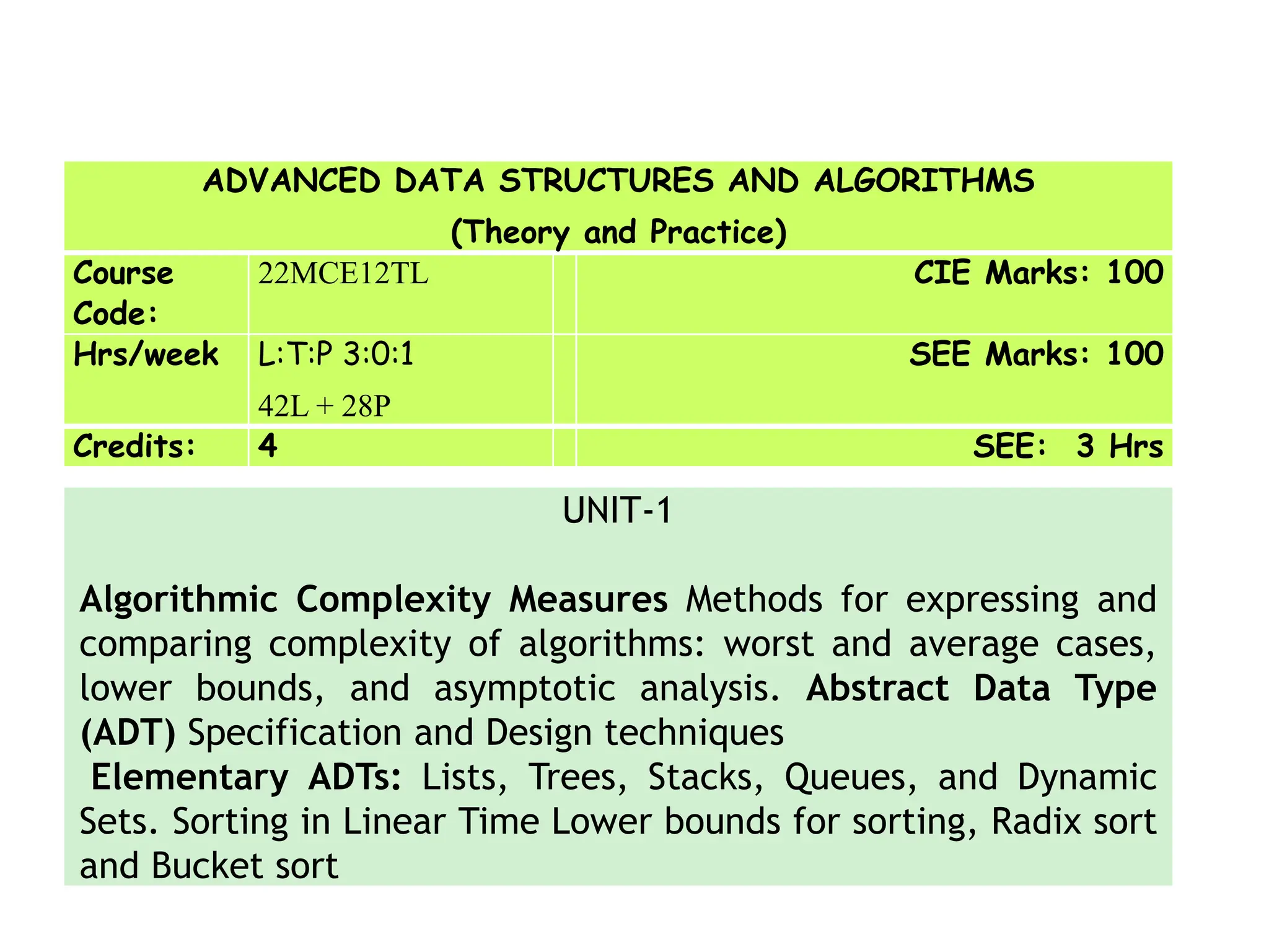
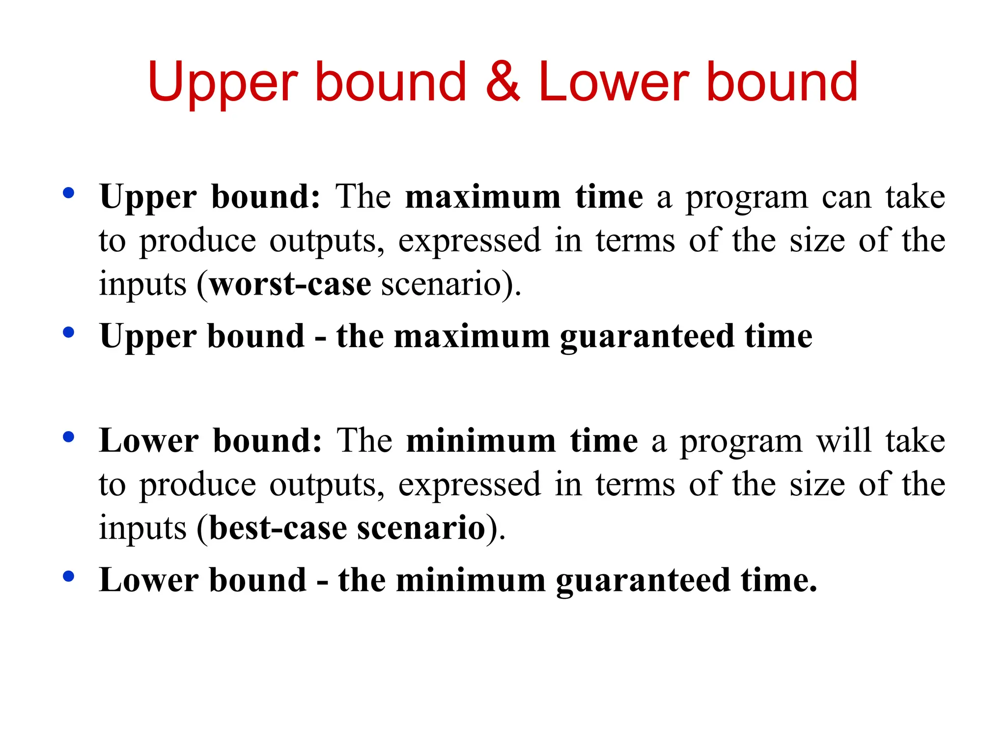
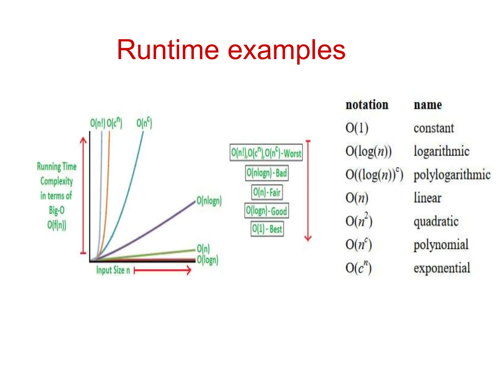
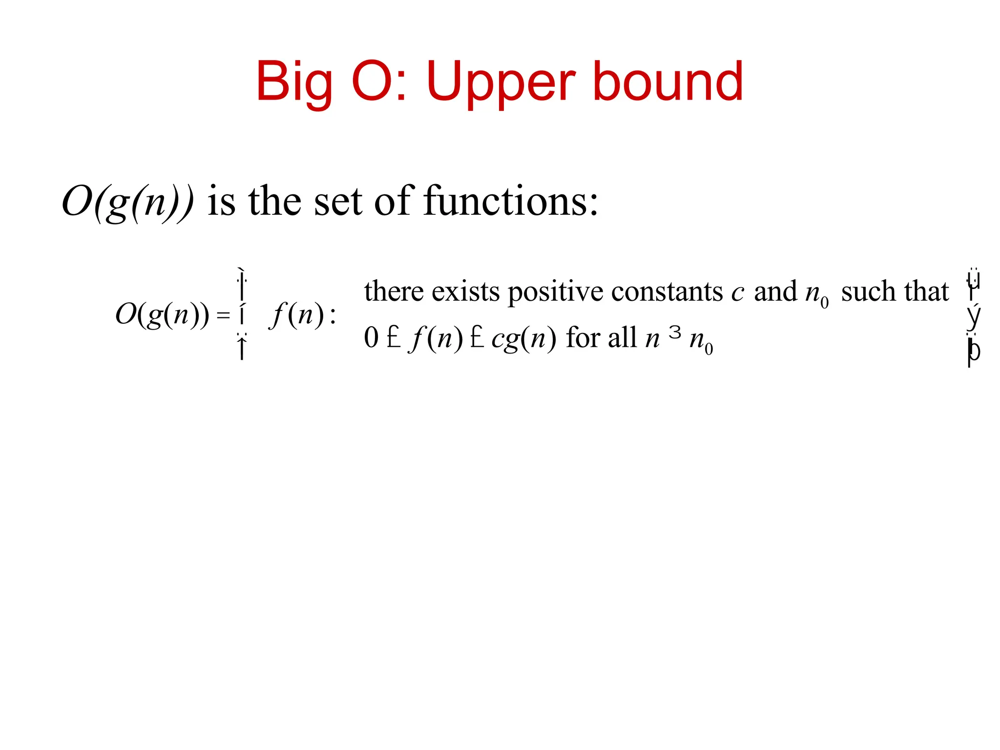
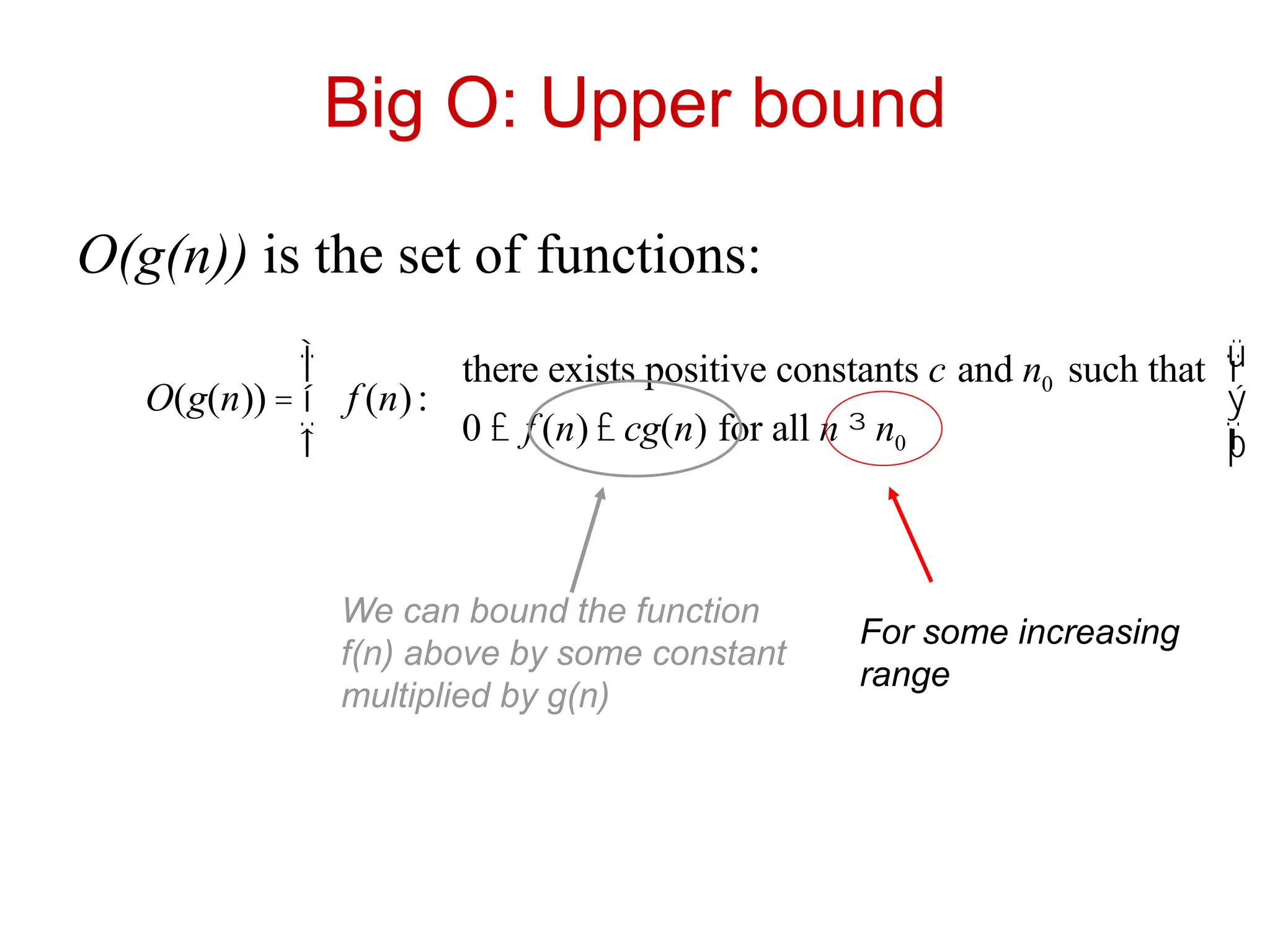
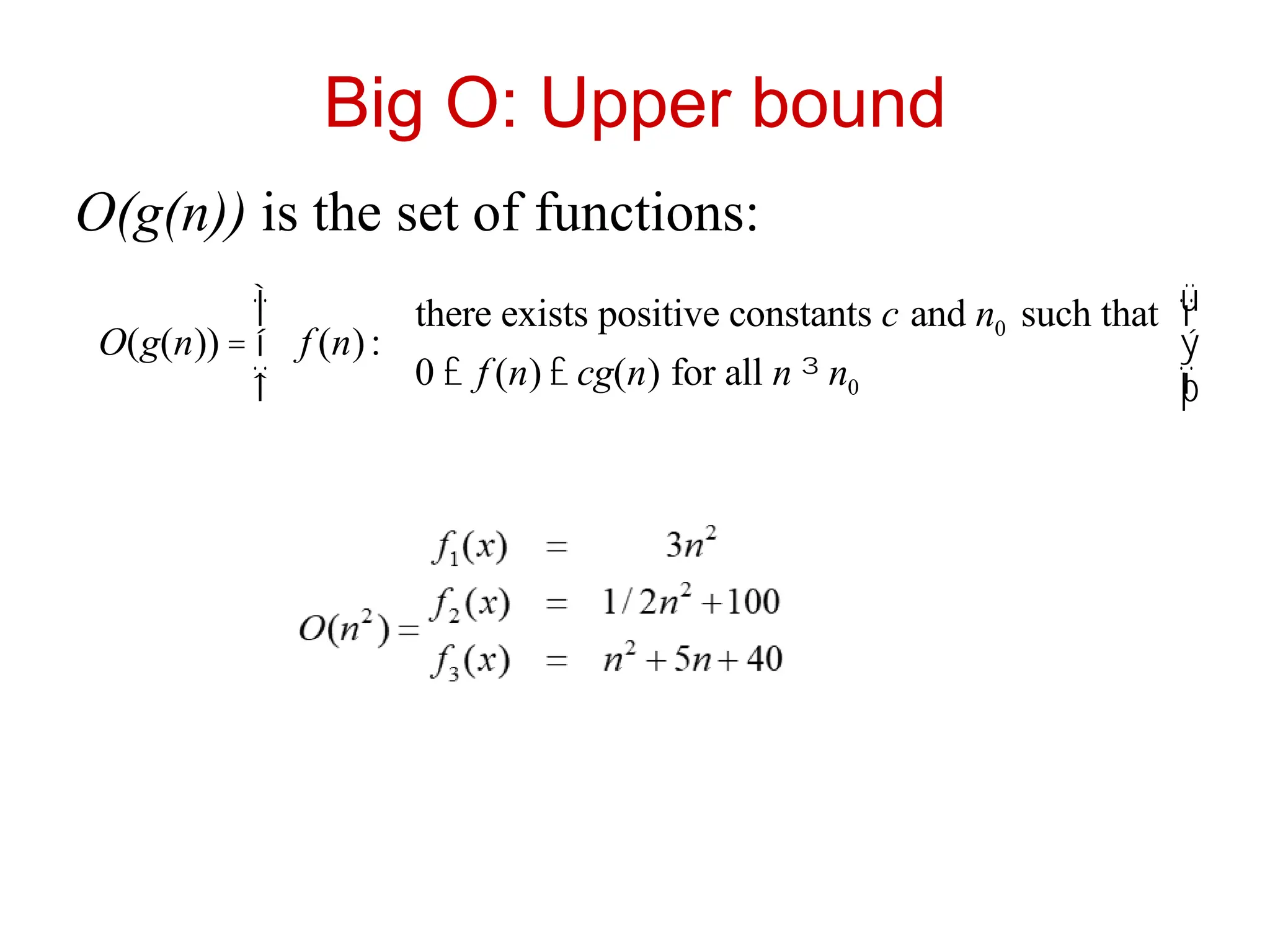
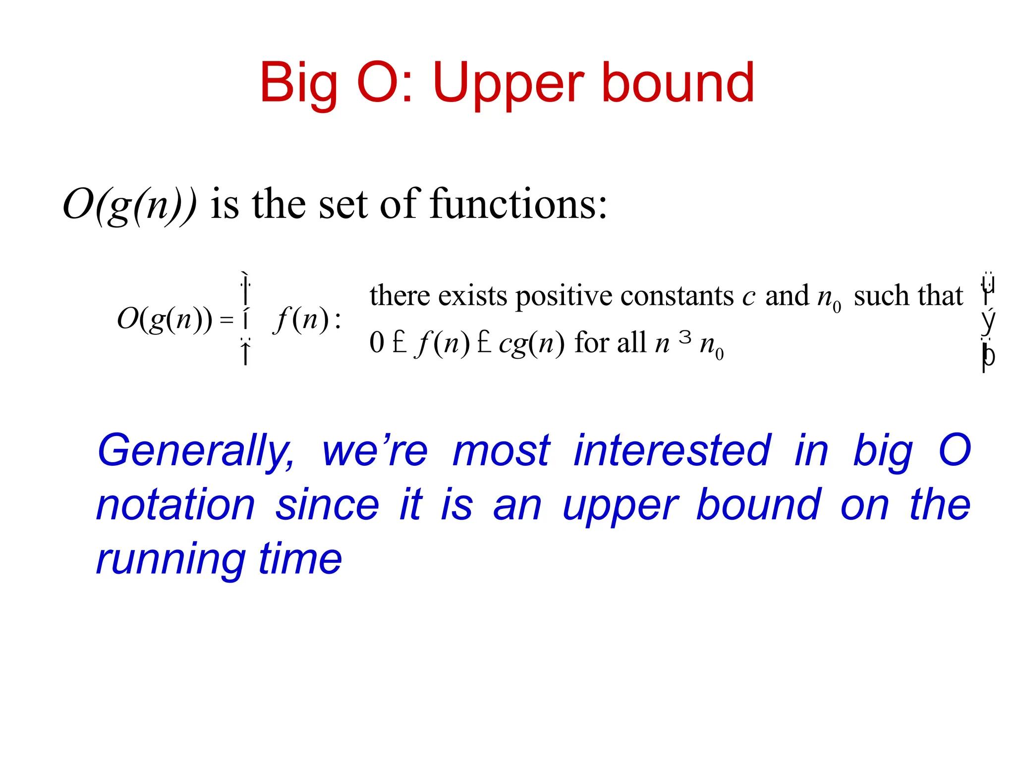
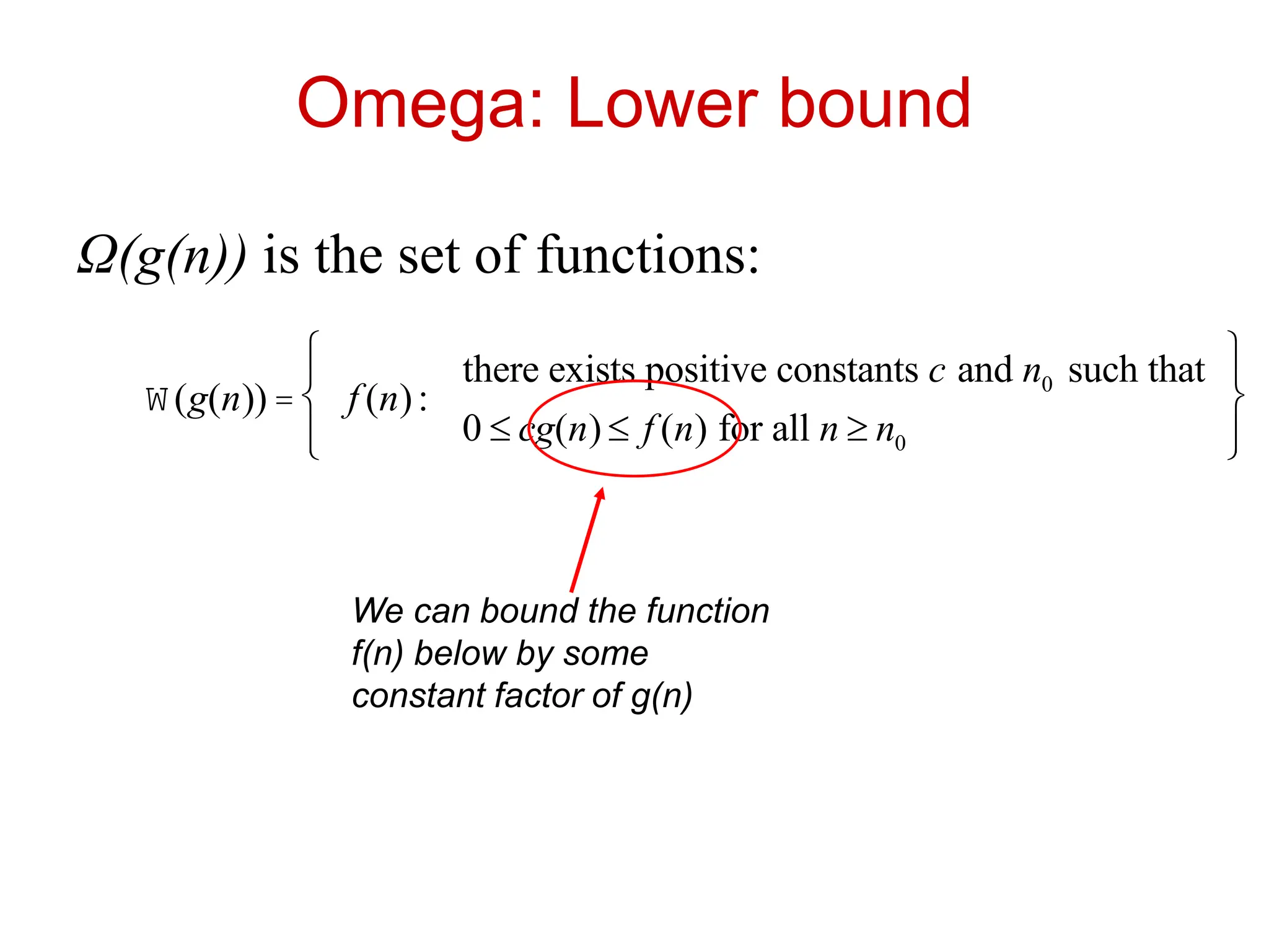
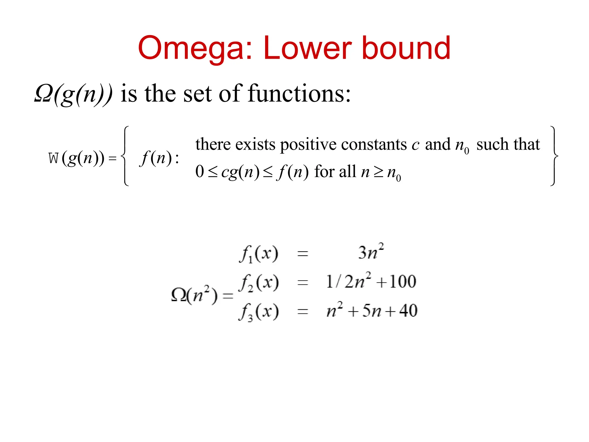
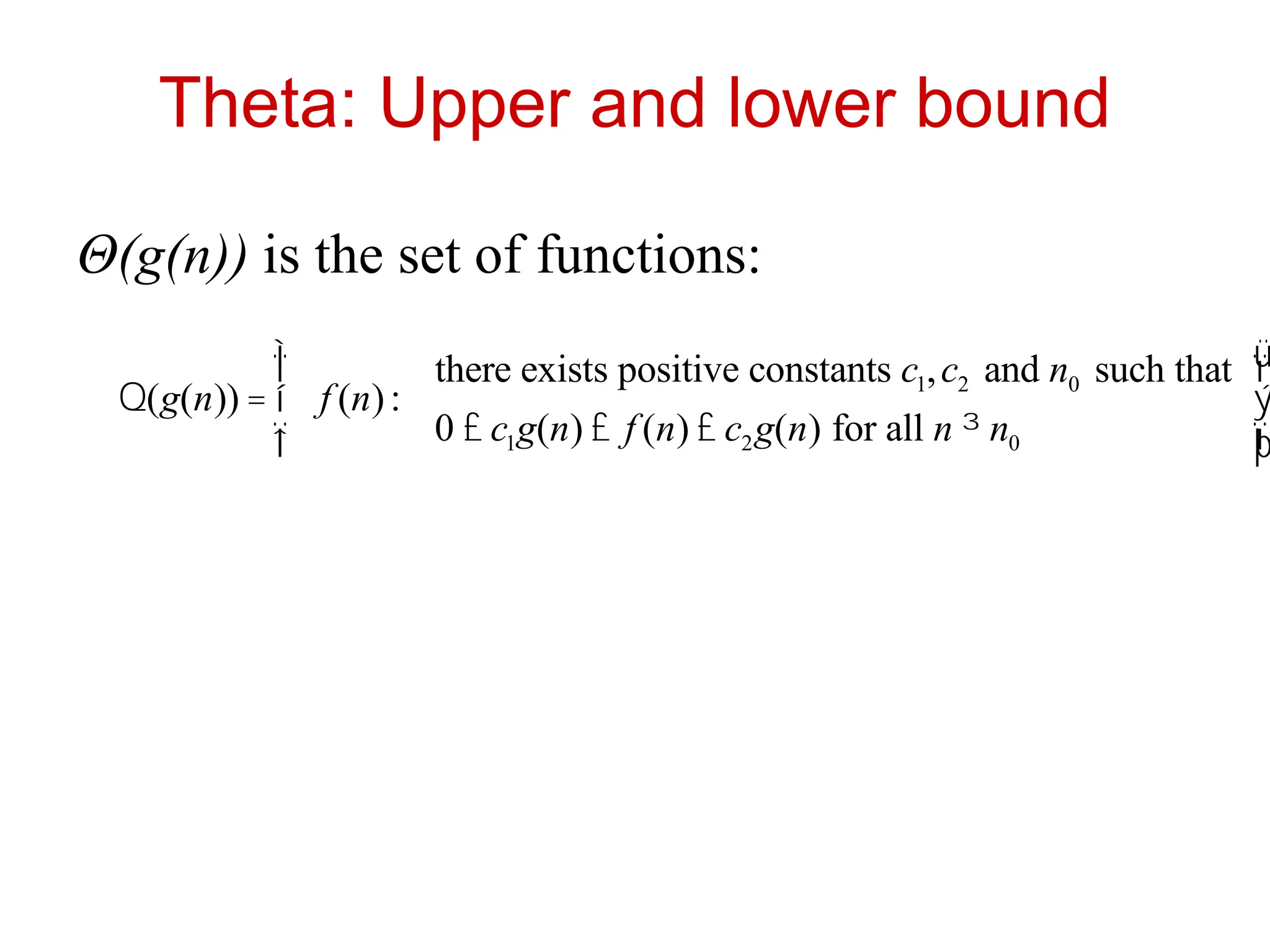
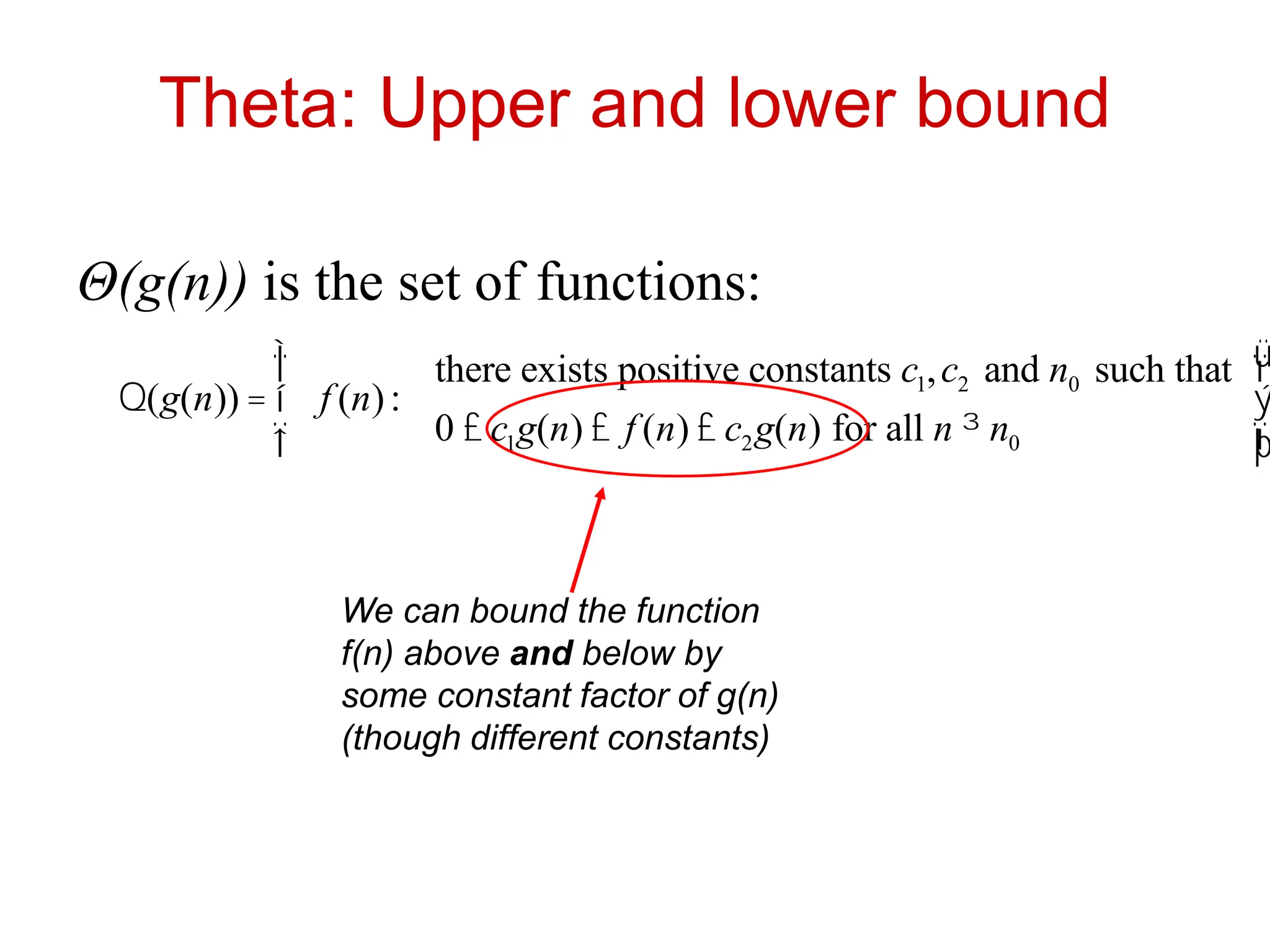
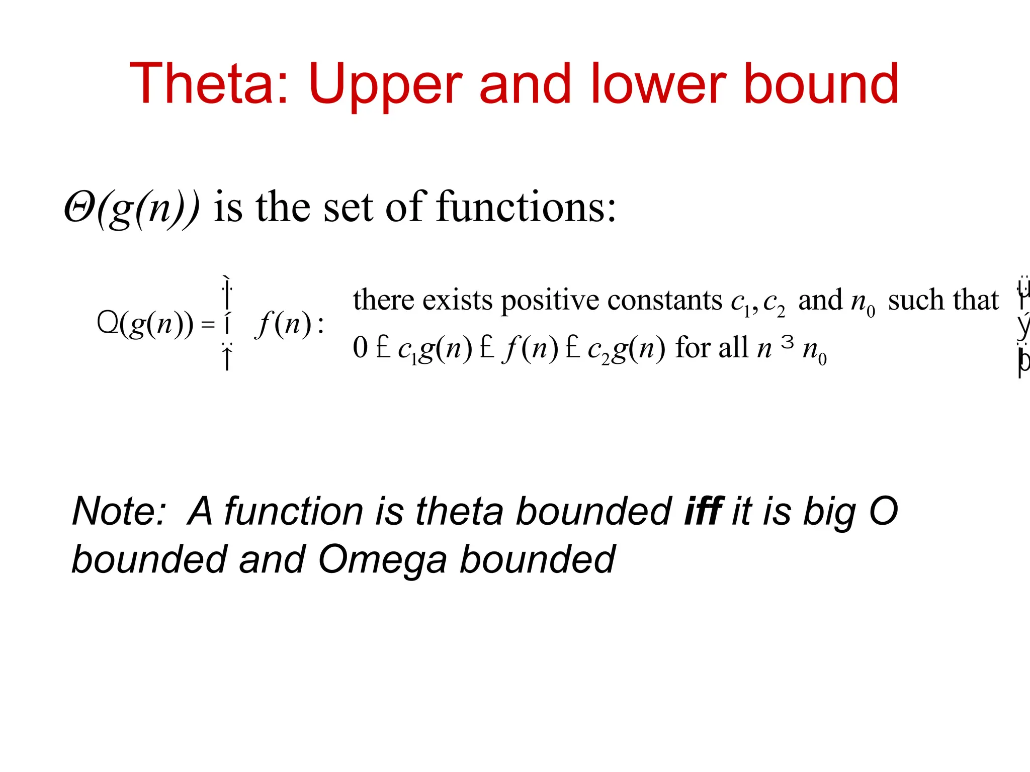
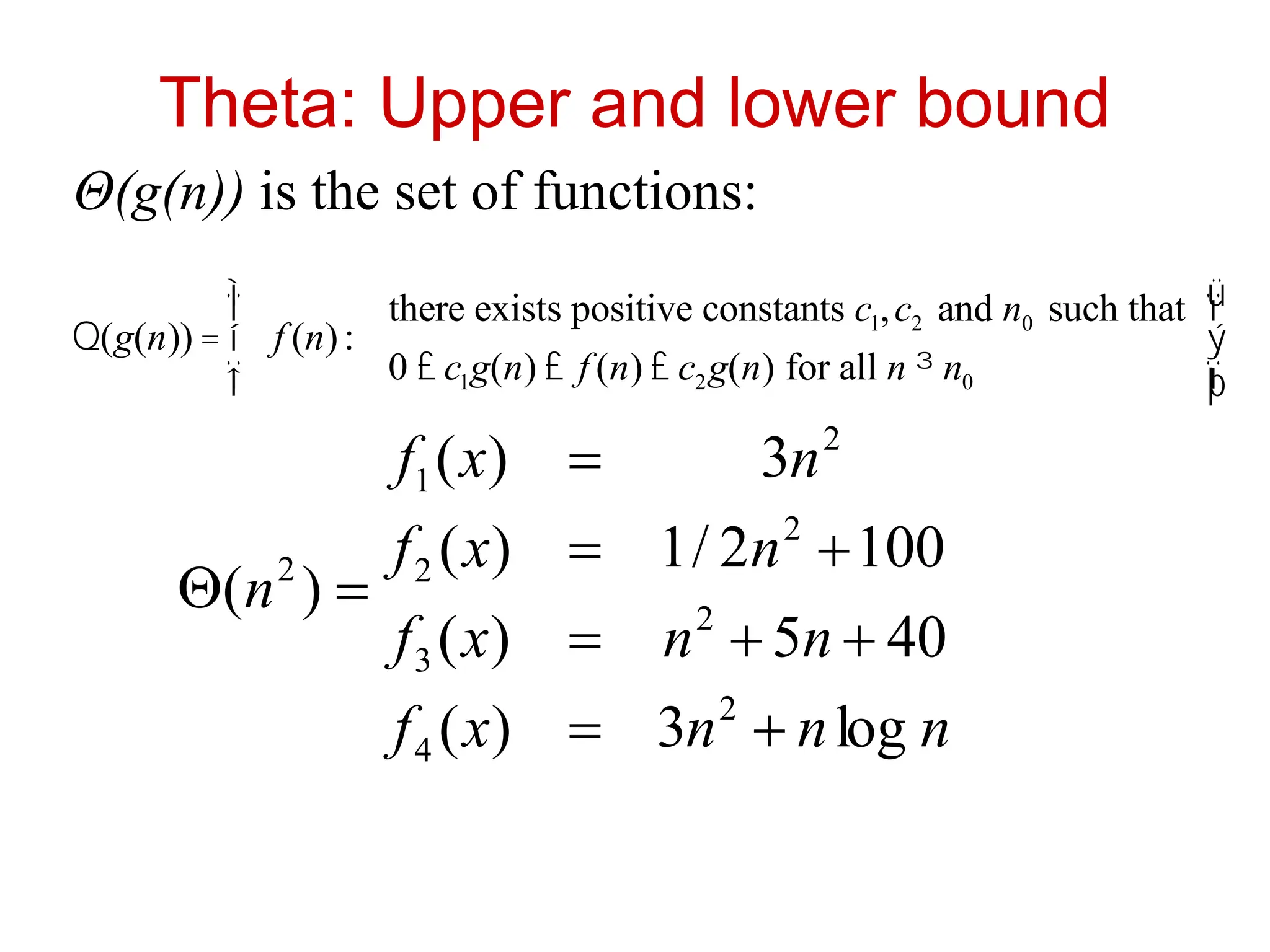
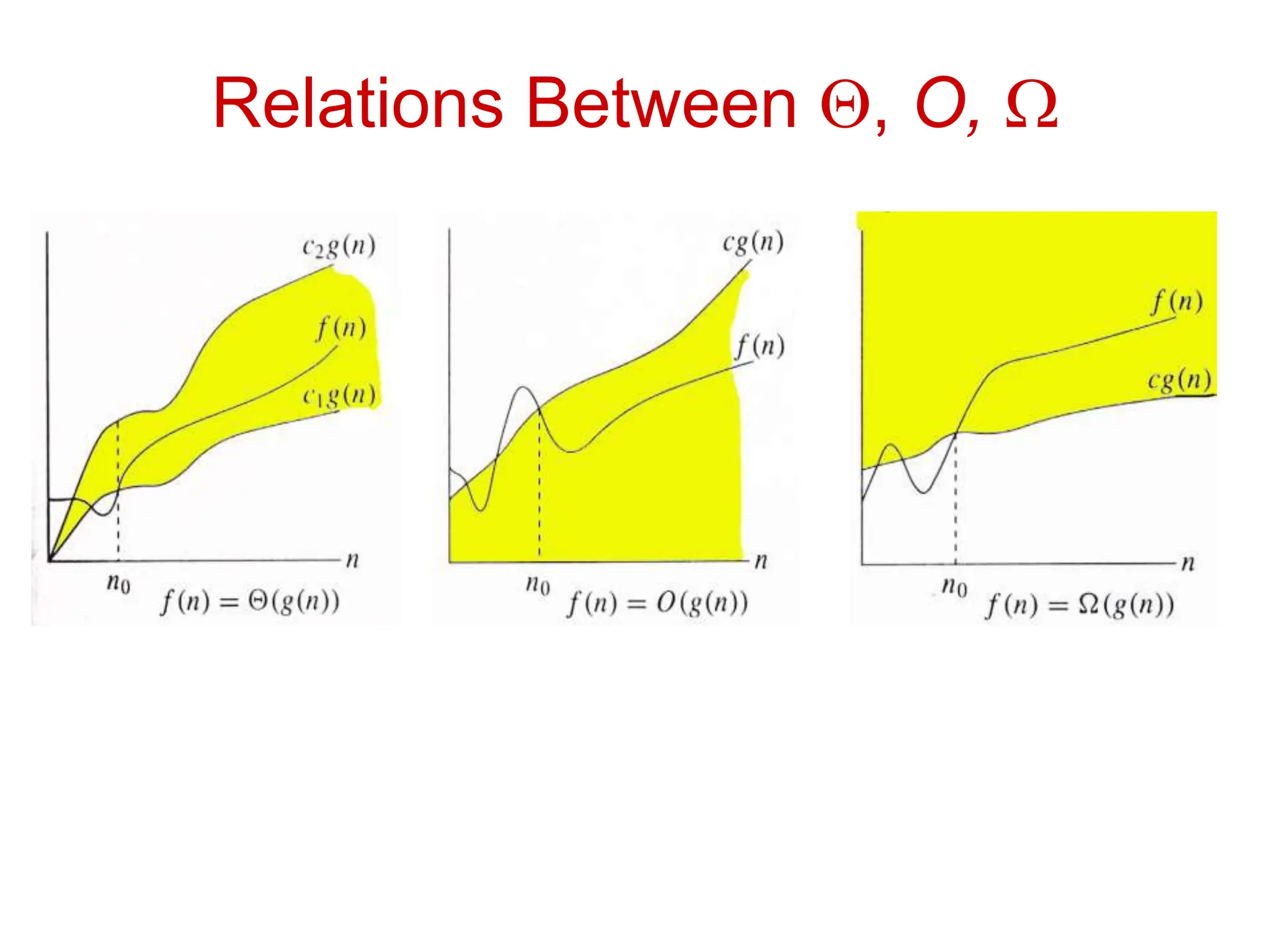
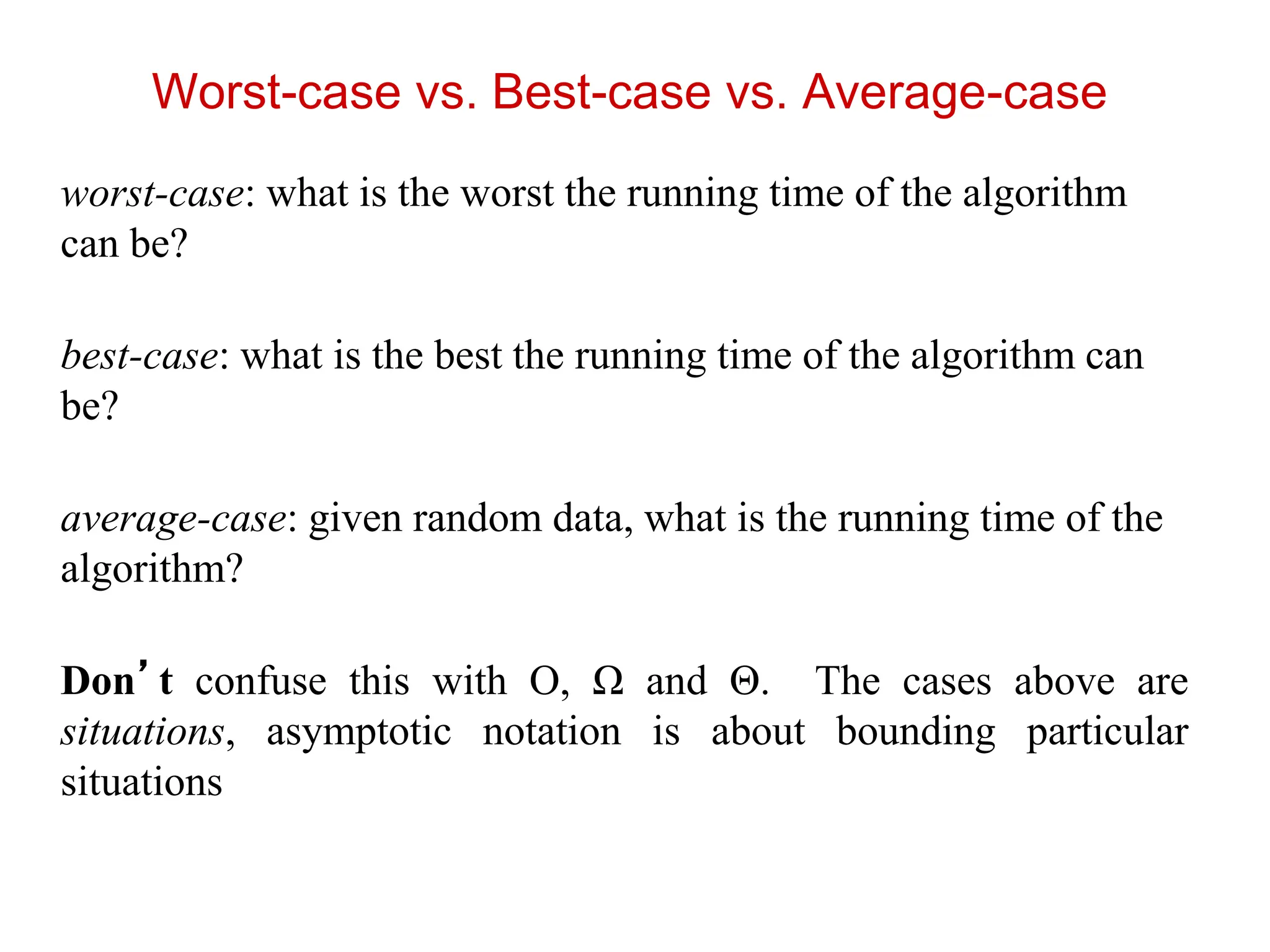
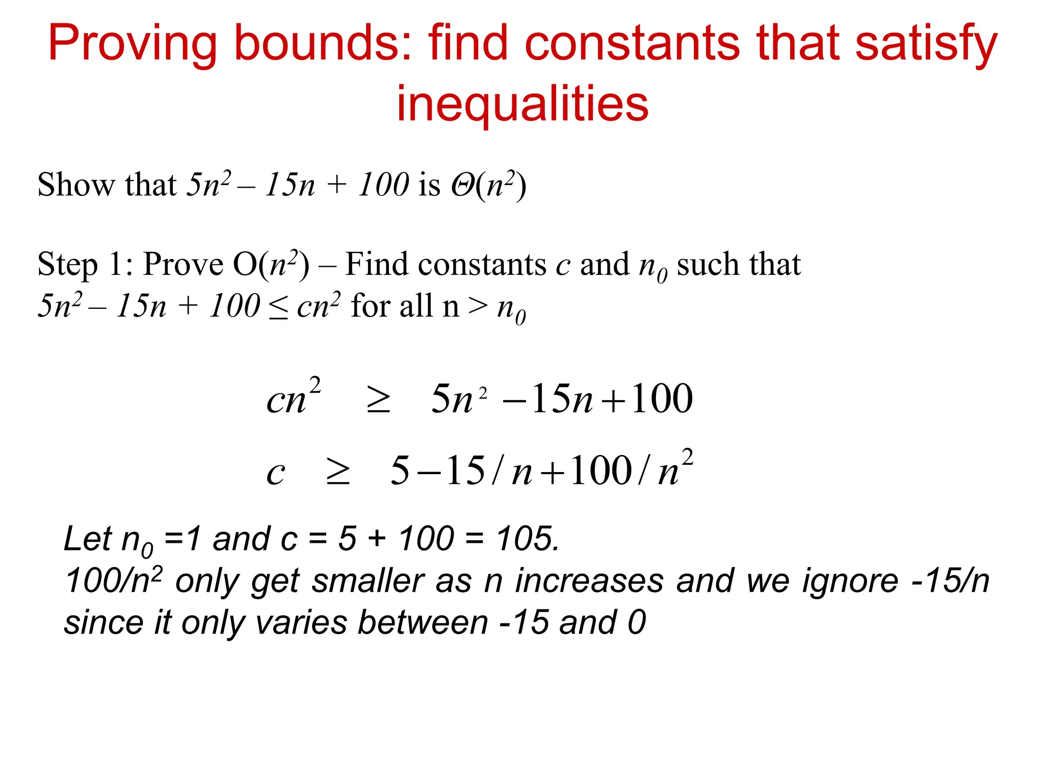
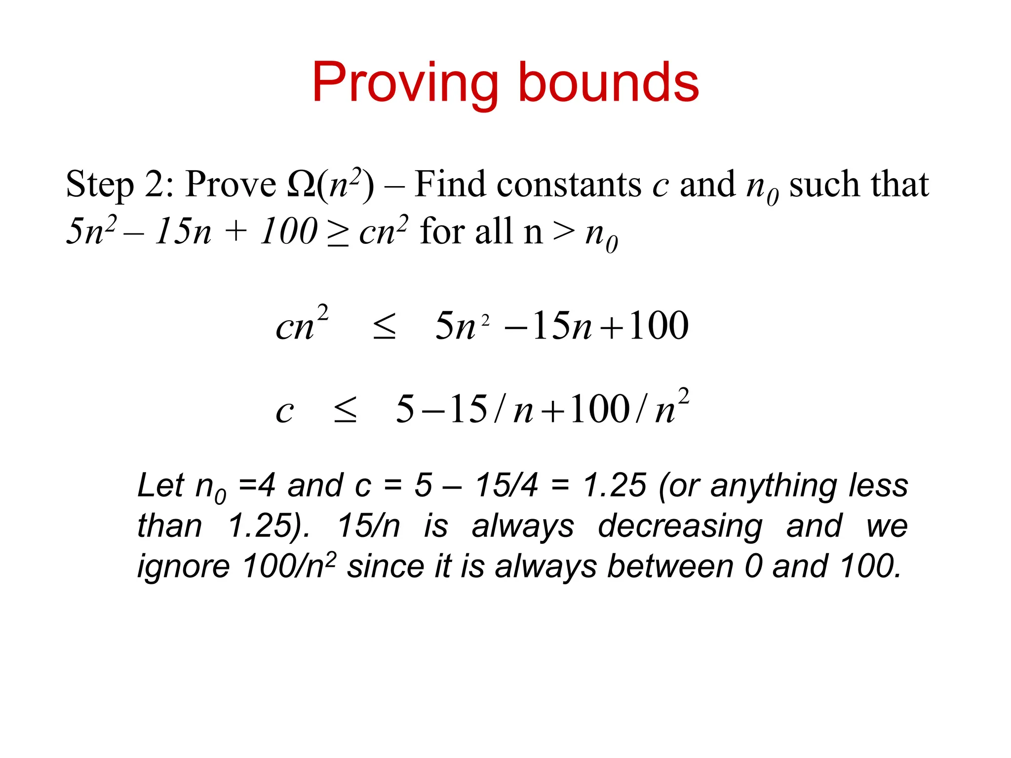
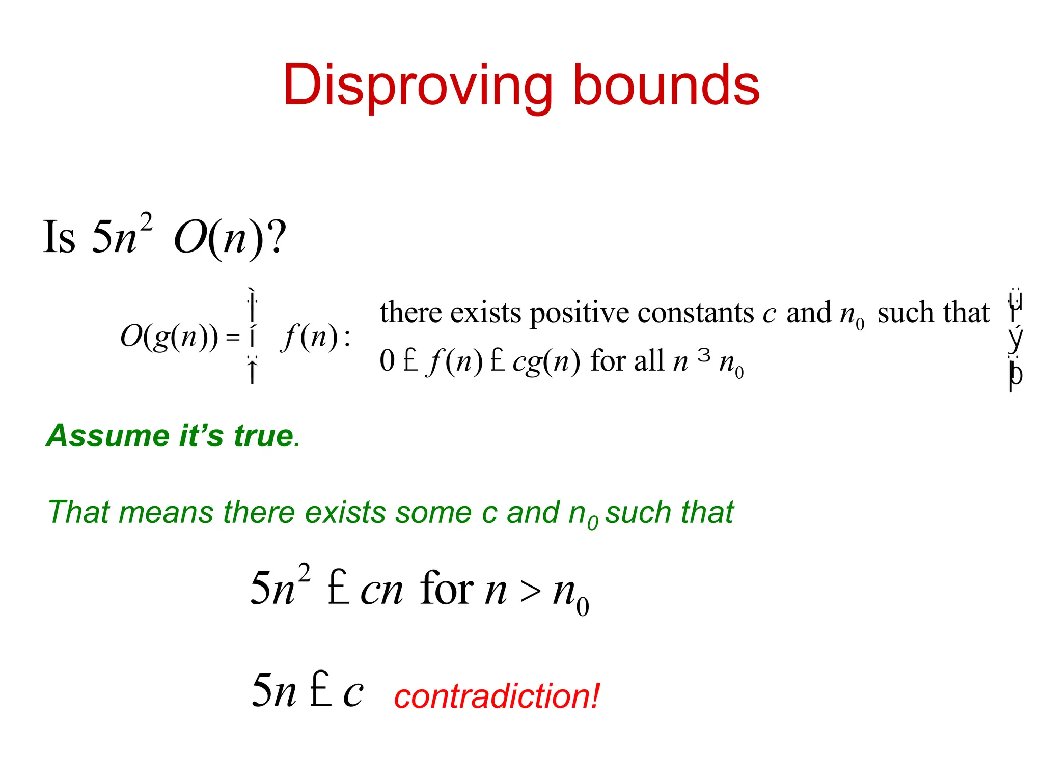
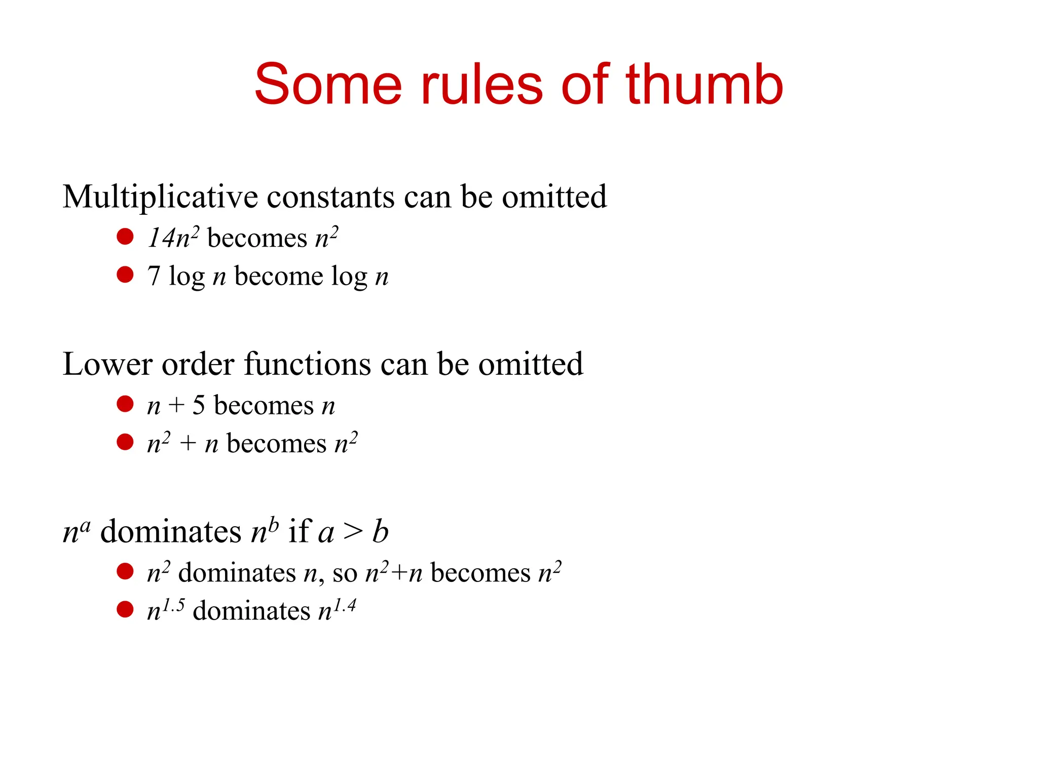
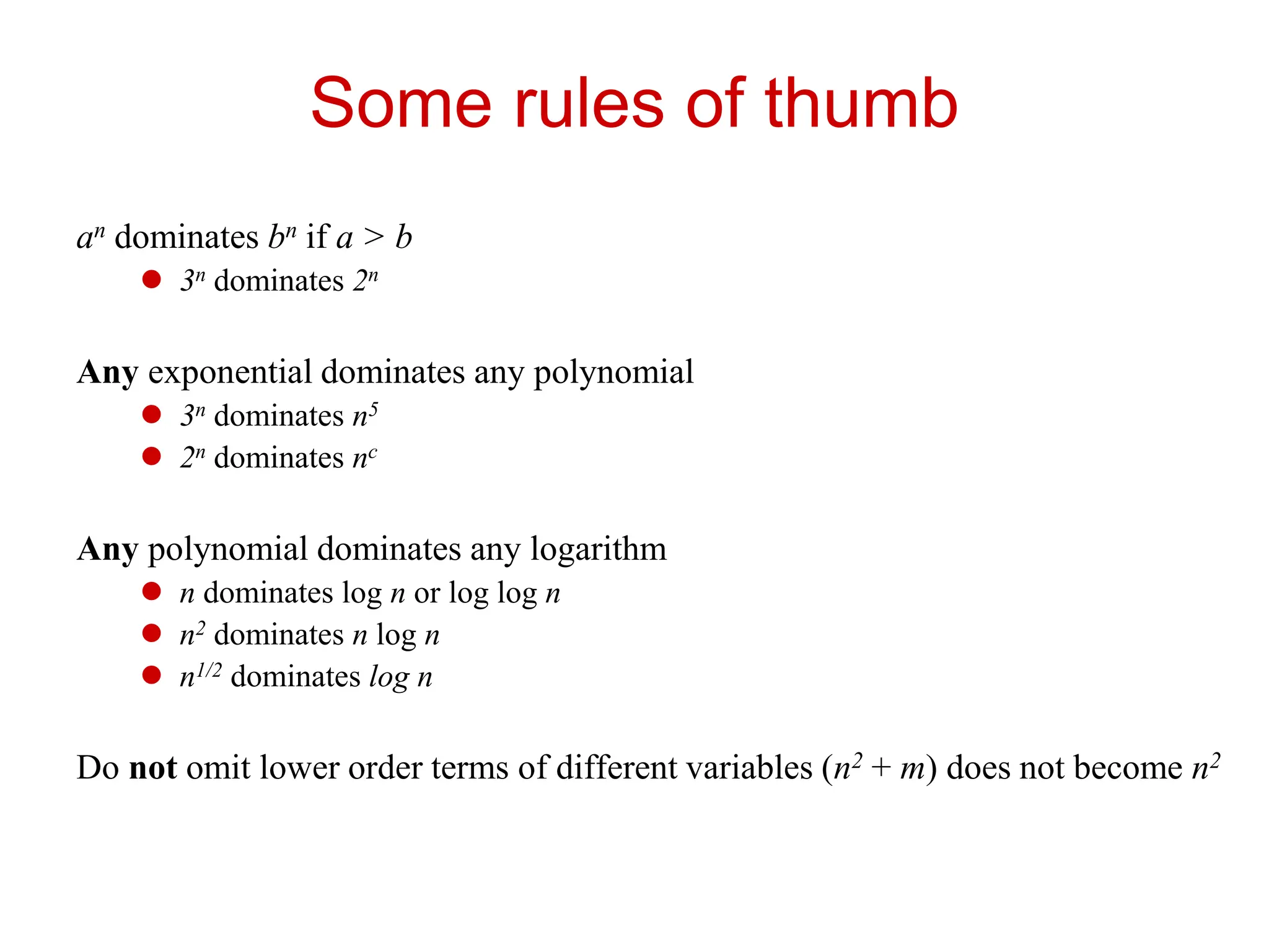
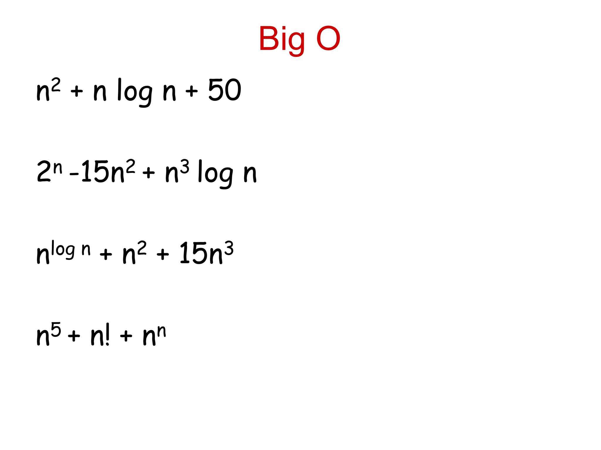
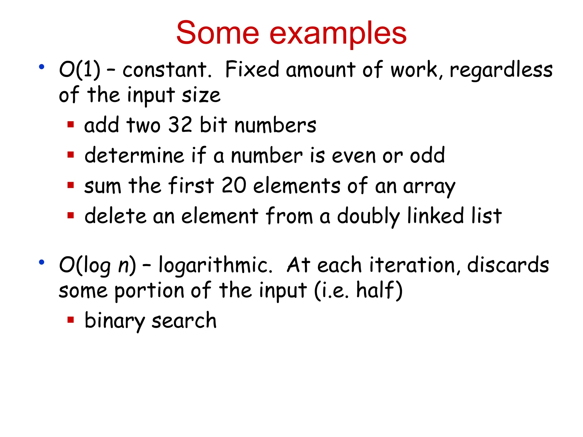
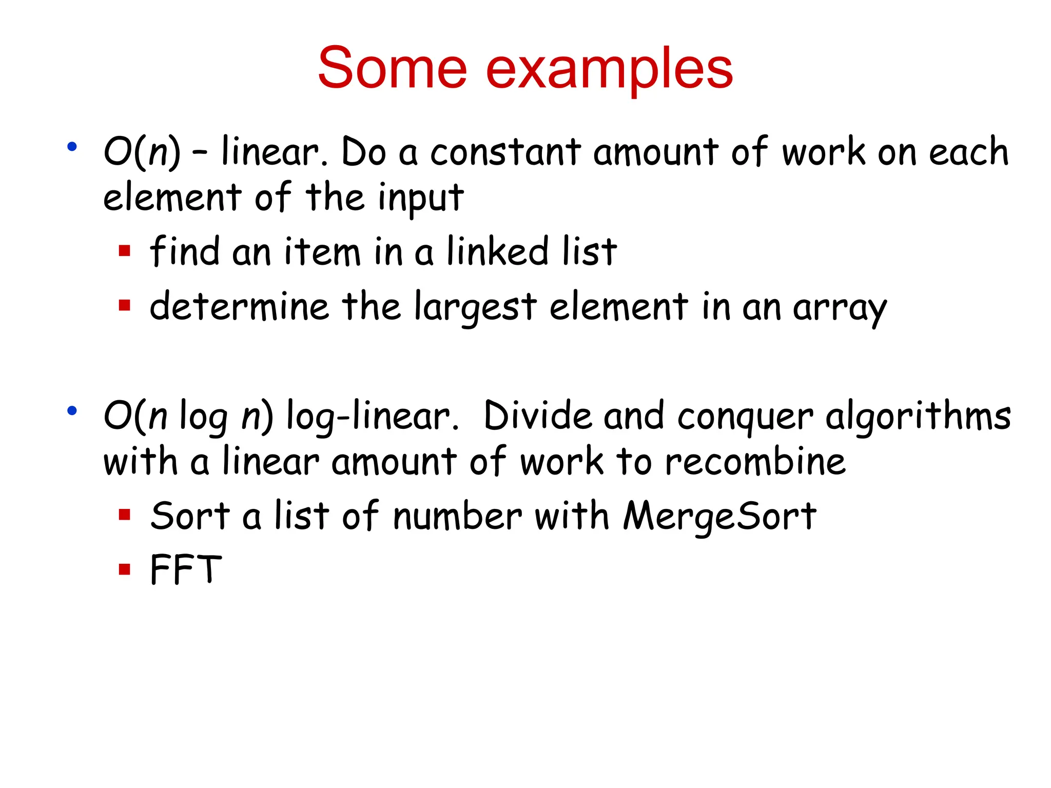
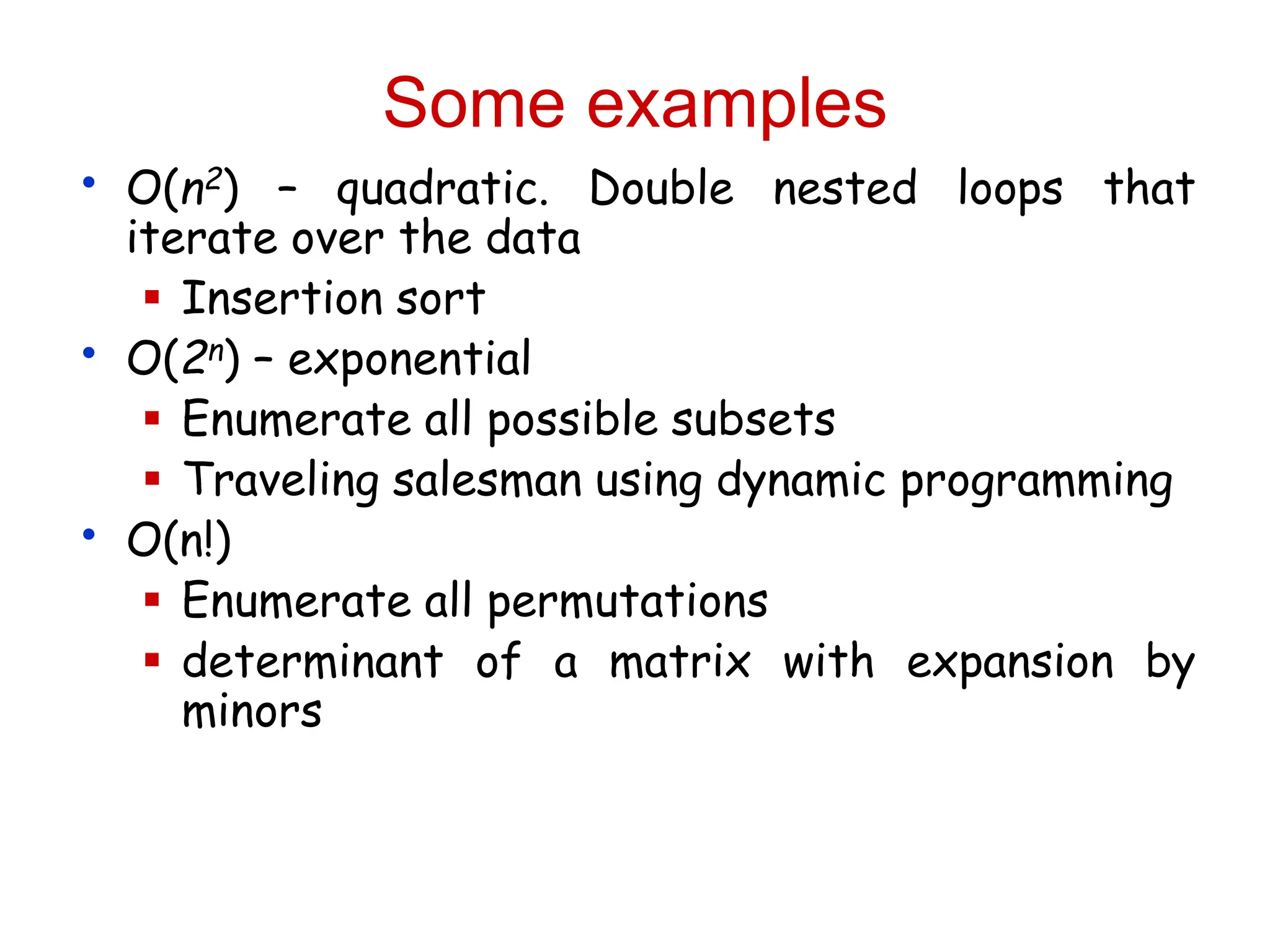
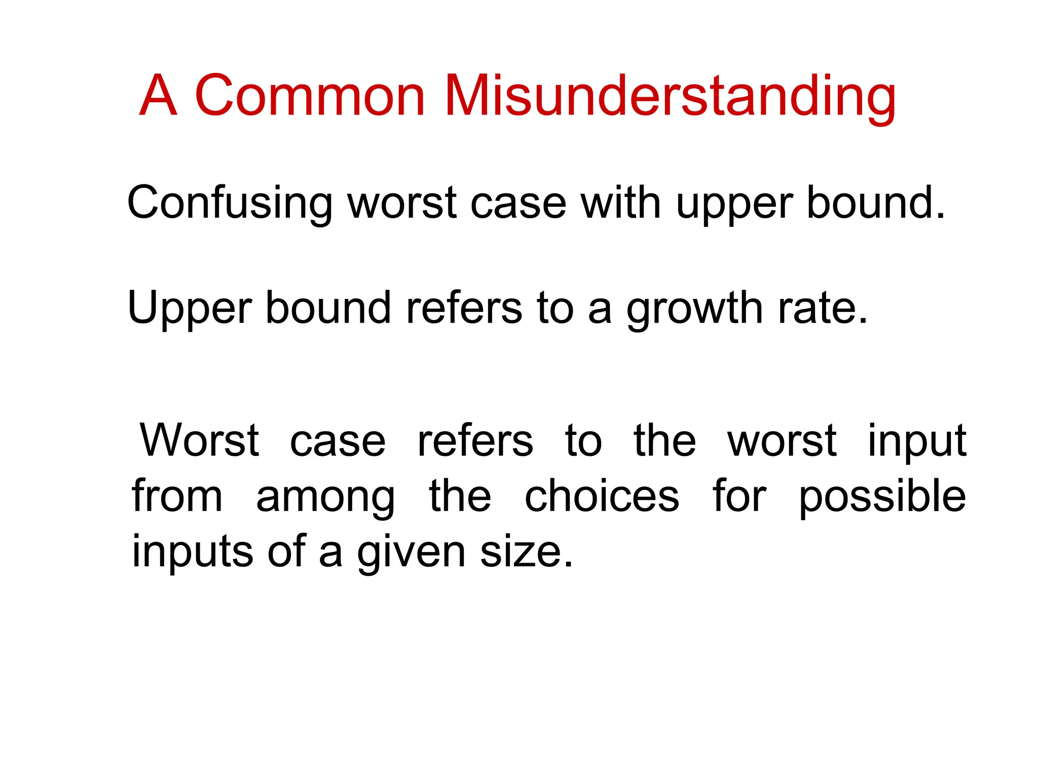
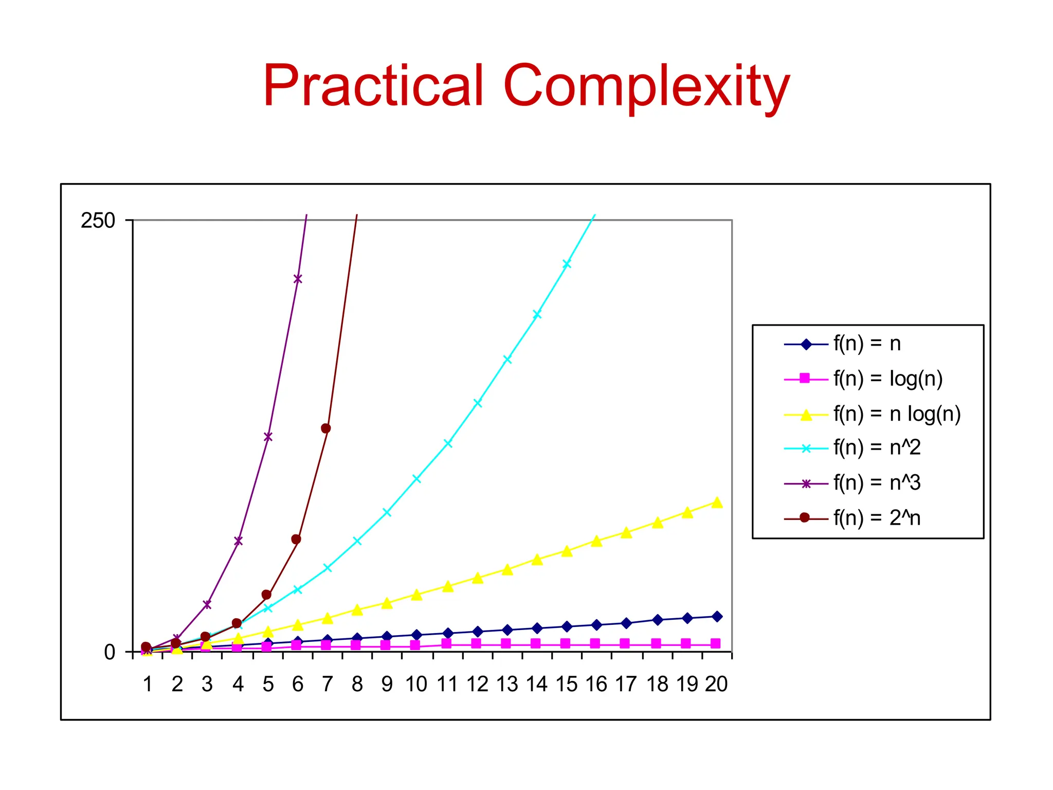
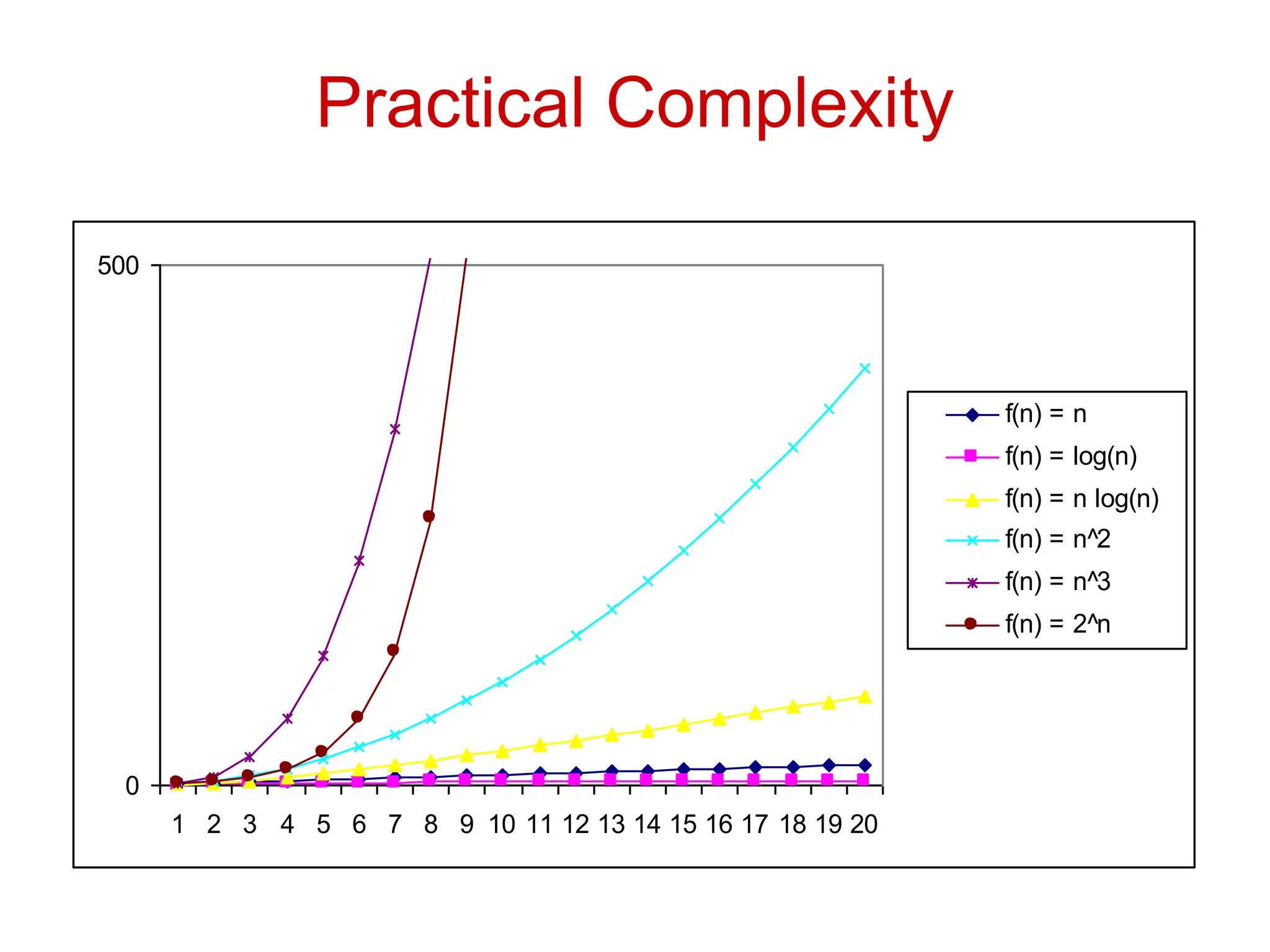
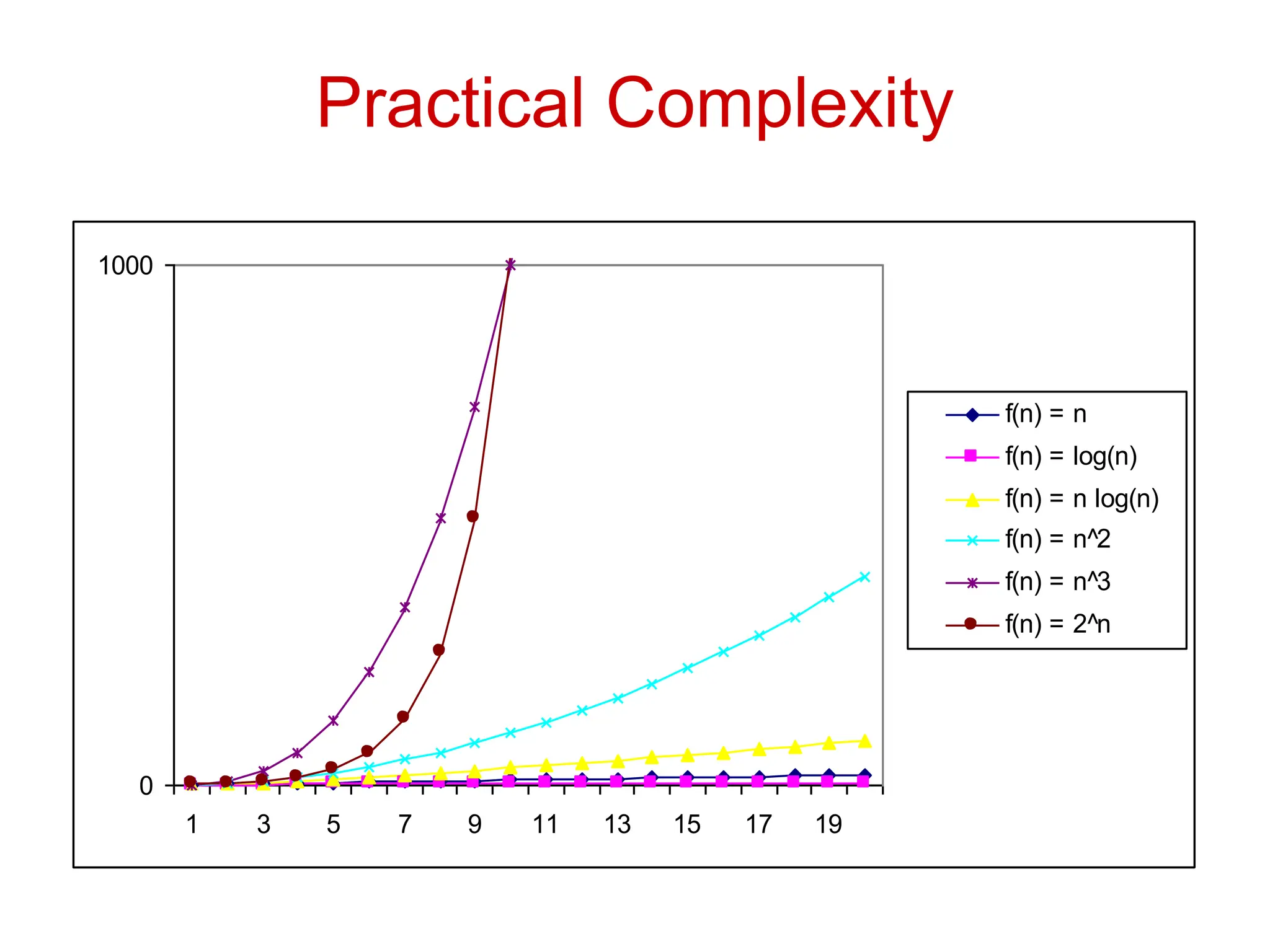
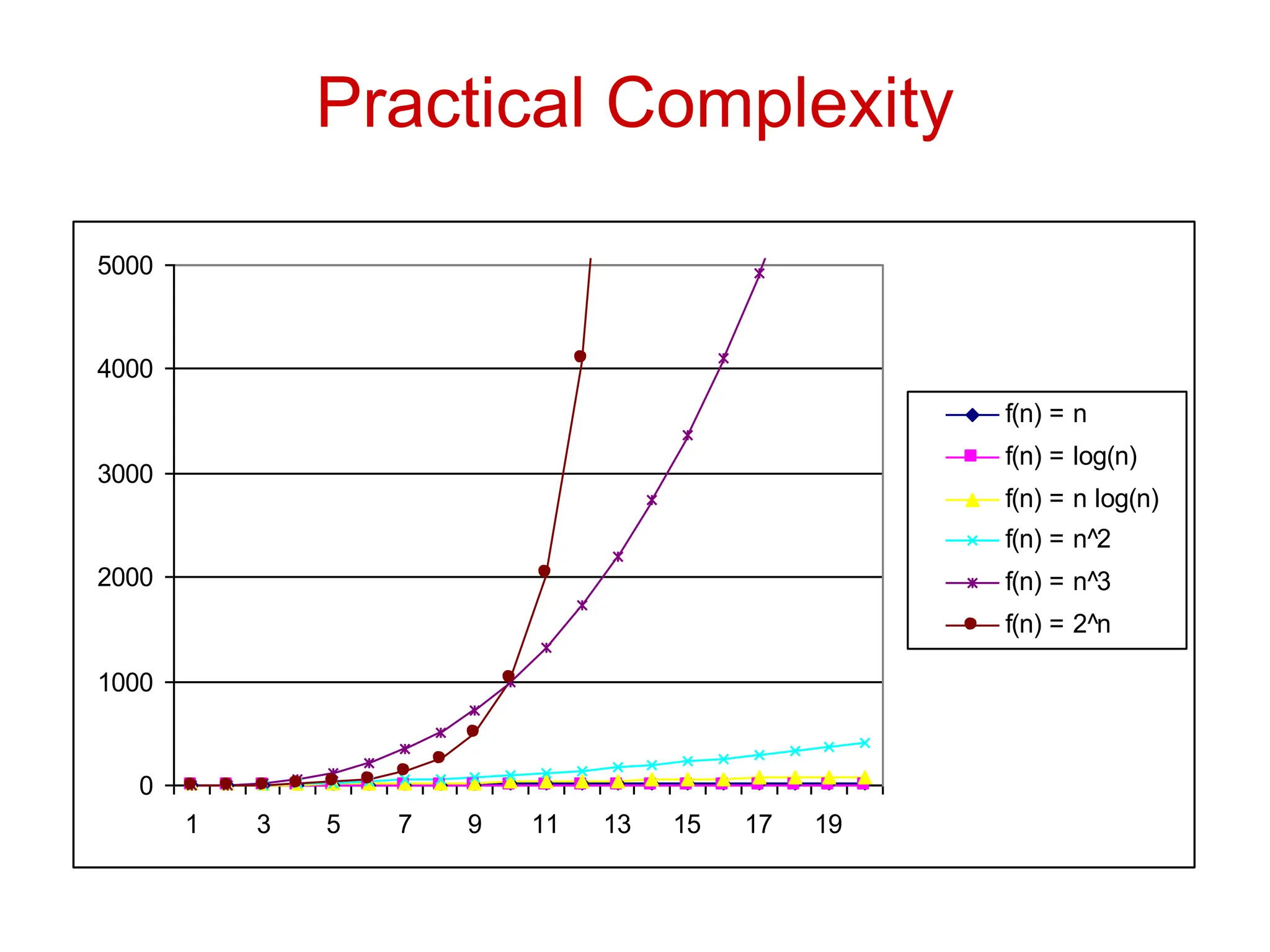
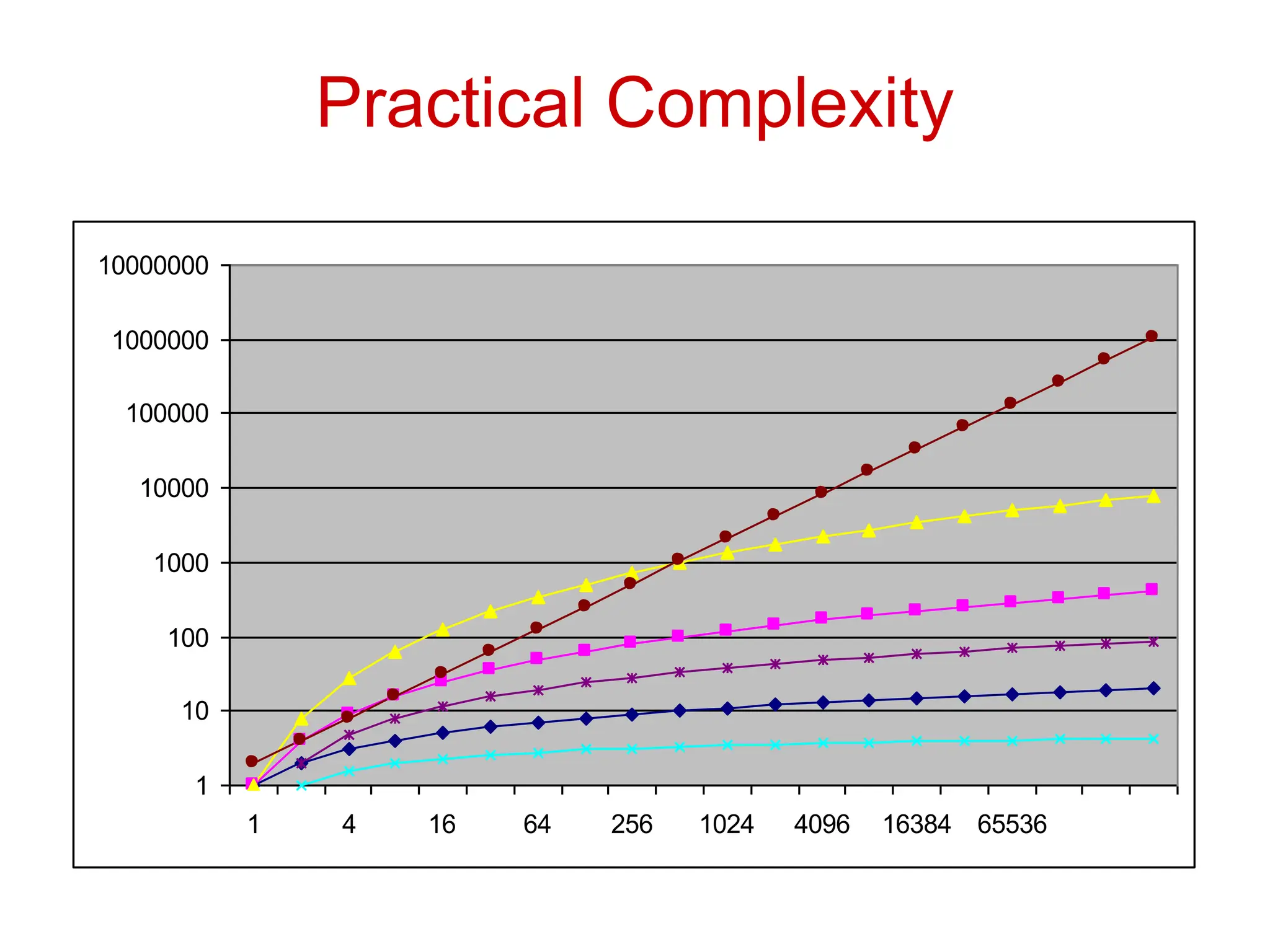
KEMBAR78
Design and analysis of algorithm ppt ppt | PPT
• x
UNIT-1
Algorithmic Complexity Measures Methods for expressing and
comparing complexity of algorithms: worst and average cases,
lower bounds, and asymptotic analysis. Abstract Data Type
(ADT) Specification and Design techniques
Elementary ADTs: Lists, Trees, Stacks, Queues, and Dynamic
Sets. Sorting in Linear Time Lower bounds for sorting, Radix sort
and Bucket sort
ADVANCED DATA STRUCTURES AND ALGORITHMS
(Theory and Practice)
Course
Code:
22MCE12TL CIE Marks: 100
Hrs/week L:T:P 3:0:1
42L + 28P
SEE Marks: 100
Credits: 4 SEE: 3 Hrs
Asymptotic Analysis
Asymptotic analysis is the process of calculating the
running time of an algorithm in mathematical units to
find the program's limitations, or “run-time
performance.”
The goal is to determine the best case, worst case and
average case time required to execute a given task.
Asymptotic Notations allow us to analyze an algorithm's
running time by identifying its behavior as the input
size for the algorithm increases
Upper bound & Lower bound
• Upper bound: The maximum time a program can take
to produce outputs, expressed in terms of the size of the
inputs (worst-case scenario).
• Upper bound - the maximum guaranteed time
• Lower bound: The minimum time a program will take
to produce outputs, expressed in terms of the size of the
inputs (best-case scenario).
• Lower bound - the minimum guaranteed time.
Asymptotic notation
Precisely calculating the actual steps is tedious and not
generally useful
Different operations take different amounts of time.
Even from run to run, things such as caching, etc. cause
variations
We want to identify categories of algorithmic runtimes
For example…
f1(n) takes n2 steps
f2(n) takes 2n + 100 steps
f3(n) takes 3n+1 steps
Which algorithm is better?
Is the difference between f2 and f3
important/significant?
Runtime examples
Big O: Upper bound
O(g(n)) is the set of functions:
O(g(n)) = f (n):
there exists positive constants c and n0 such that
0 £ f (n) £ cg(n) for all n ³ n0
ì
í
ï
î
ï
ü
ý
ï
þ
ï
Big O: Upper bound
O(g(n)) is the set of functions:
O(g(n)) = f (n):
there exists positive constants c and n0 such that
0 £ f (n) £ cg(n) for all n ³ n0
ì
í
ï
î
ï
ü
ý
ï
þ
ï
We can bound the function
f(n) above by some constant
factor of g(n)
Big O: Upper bound
O(g(n)) is the set of functions:
O(g(n)) = f (n):
there exists positive constants c and n0 such that
0 £ f (n) £ cg(n) for all n ³ n0
ì
í
ï
î
ï
ü
ý
ï
þ
ï
We can bound the function
f(n) above by some constant
multiplied by g(n)
For some increasing
range
Big O: Upper bound
O(g(n)) is the set of functions:
O(g(n)) = f (n):
there exists positive constants c and n0 such that
0 £ f (n) £ cg(n) for all n ³ n0
ì
í
ï
î
ï
ü
ý
ï
þ
ï
Big O: Upper bound
O(g(n)) is the set of functions:
O(g(n)) = f (n):
there exists positive constants c and n0 such that
0 £ f (n) £ cg(n) for all n ³ n0
ì
í
ï
î
ï
ü
ý
ï
þ
ï
Generally, we’re most interested in big O
notation since it is an upper bound on the
running time
Omega: Lower bound
Ω(g(n)) is the set of functions:
W(g(n)) = f (n):
there exists positive constants c and n0 such that
0 £ cg(n) £ f (n) for all n ³ n0
ì
í
ï
î
ï
ü
ý
ï
þ
ï
Omega: Lower bound
Ω(g(n)) is the set of functions:
W(g(n)) = f (n):
there exists positive constants c and n0 such that
0 £ cg(n) £ f (n) for all n ³ n0
ì
í
ï
î
ï
ü
ý
ï
þ
ï
We can bound the function
f(n) below by some
constant factor of g(n)
Omega: Lower bound
Ω(g(n)) is the set of functions:
W(g(n)) = f (n):
there exists positive constants c and n0 such that
0 £ cg(n) £ f (n) for all n ³ n0
ì
í
ï
î
ï
ü
ý
ï
þ
ï
Theta: Upper and lower bound
Θ(g(n)) is the set of functions:
Q(g(n)) = f (n):
there exists positive constants c1,c2 and n0 such that
0 £ c1g(n) £ f (n) £ c2g(n) for all n ³ n0
ì
í
ï
î
ï
ü
ý
ï
þ
ï
Theta: Upper and lower bound
Θ(g(n)) is the set of functions:
Q(g(n)) = f (n):
there exists positive constants c1,c2 and n0 such that
0 £ c1g(n) £ f (n) £ c2g(n) for all n ³ n0
ì
í
ï
î
ï
ü
ý
ï
þ
ï
We can bound the function
f(n) above and below by
some constant factor of g(n)
(though different constants)
Theta: Upper and lower bound
Θ(g(n)) is the set of functions:
Q(g(n)) = f (n):
there exists positive constants c1,c2 and n0 such that
0 £ c1g(n) £ f (n) £ c2g(n) for all n ³ n0
ì
í
ï
î
ï
ü
ý
ï
þ
ï
Note: A function is theta bounded iff it is big O
bounded and Omega bounded
Theta: Upper and lower bound
Θ(g(n)) is the set of functions:
Q(g(n)) = f (n):
there exists positive constants c1,c2 and n0 such that
0 £ c1g(n) £ f (n) £ c2g(n) for all n ³ n0
ì
í
ï
î
ï
ü
ý
ï
þ
ï
n
n
n
x
f
n
n
x
f
n
x
f
n
x
f
n
log
3
)
(
40
5
)
(
100
2
/
1
)
(
3
)
(
)
(
2
4
2
3
2
2
2
1
2










Visually
f(n)
Visually: upper bound
n0
f(n)
Visually: lower bound
n0
f(n)
Relations Between , O, W
Worst-case vs. Best-case vs. Average-case
worst-case: what is the worst the running time of the algorithm
can be?
best-case: what is the best the running time of the algorithm can
be?
average-case: given random data, what is the running time of the
algorithm?
Don’t confuse this with O, Ω and Θ. The cases above are
situations, asymptotic notation is about bounding particular
situations
Proving bounds: find constants that satisfy
inequalities
Show that 5n2 – 15n + 100 is Θ(n2)
Step 1: Prove O(n2) – Find constants c and n0 such that
5n2 – 15n + 100 ≤ cn2 for all n > n0
100
15
5 2
2


 n
n
cn
2
/
100
/
15
5 n
n
c 


Let n0 =1 and c = 5 + 100 = 105.
100/n2 only get smaller as n increases and we ignore -15/n
since it only varies between -15 and 0
Proving bounds
Step 2: Prove Ω(n2) – Find constants c and n0 such that
5n2 – 15n + 100 ≥ cn2 for all n > n0
100
15
5 2
2


 n
n
cn
2
/
100
/
15
5 n
n
c 


Let n0 =4 and c = 5 – 15/4 = 1.25 (or anything less
than 1.25). 15/n is always decreasing and we
ignore 100/n2 since it is always between 0 and 100.
Bounds
Is 5n2
O(n)? No
How would we prove it?
O(g(n)) = f (n):
there exists positive constants c and n0 such that
0 £ f (n) £ cg(n) for all n ³ n0
ì
í
ï
î
ï
ü
ý
ï
þ
ï
Disproving bounds
Is 5n2
O(n)?
O(g(n)) = f (n):
there exists positive constants c and n0 such that
0 £ f (n) £ cg(n) for all n ³ n0
ì
í
ï
î
ï
ü
ý
ï
þ
ï
Assume it’s true.
That means there exists some c and n0 such that
5n2
£ cn for n > n0
5n £ c contradiction!
Some rules of thumb
Multiplicative constants can be omitted
 14n2 becomes n2
 7 log n become log n
Lower order functions can be omitted
 n + 5 becomes n
 n2 + n becomes n2
na dominates nb if a > b
 n2 dominates n, so n2+n becomes n2
 n1.5 dominates n1.4
Some rules of thumb
an dominates bn if a > b
 3n dominates 2n
Any exponential dominates any polynomial
 3n dominates n5
 2n dominates nc
Any polynomial dominates any logarithm
 n dominates log n or log log n
 n2 dominates n log n
 n1/2 dominates log n
Do not omit lower order terms of different variables (n2 + m) does not become n2
Big O
n2 + n log n + 50
2n -15n2 + n3 log n
nlog n + n2 + 15n3
n5 + n! + nn
Some examples
• O(1) – constant. Fixed amount of work, regardless
of the input size
 add two 32 bit numbers
 determine if a number is even or odd
 sum the first 20 elements of an array
 delete an element from a doubly linked list
• O(log n) – logarithmic. At each iteration, discards
some portion of the input (i.e. half)
 binary search
Some examples
• O(n) – linear. Do a constant amount of work on each
element of the input
 find an item in a linked list
 determine the largest element in an array
• O(n log n) log-linear. Divide and conquer algorithms
with a linear amount of work to recombine
 Sort a list of number with MergeSort
 FFT
Some examples
• O(n2) – quadratic. Double nested loops that
iterate over the data
 Insertion sort
• O(2n) – exponential
 Enumerate all possible subsets
 Traveling salesman using dynamic programming
• O(n!)
 Enumerate all permutations
 determinant of a matrix with expansion by
minors
A Common Misunderstanding
Confusing worst case with upper bound.
Upper bound refers to a growth rate.
Worst case refers to the worst input
from among the choices for possible
inputs of a given size.
Practical Complexity
0
250
1 2 3 4 5 6 7 8 9 10 11 12 13 14 15 16 17 18 19 20
f(n) = n
f(n) = log(n)
f(n) = n log(n)
f(n) = n^2
f(n) = n^3
f(n) = 2^n
Practical Complexity
0
500
1 2 3 4 5 6 7 8 9 10 11 12 13 14 15 16 17 18 19 20
f(n) = n
f(n) = log(n)
f(n) = n log(n)
f(n) = n^2
f(n) = n^3
f(n) = 2^n
Practical Complexity
0
1000
1 3 5 7 9 11 13 15 17 19
f(n) = n
f(n) = log(n)
f(n) = n log(n)
f(n) = n^2
f(n) = n^3
f(n) = 2^n
Practical Complexity
0
1000
2000
3000
4000
5000
1 3 5 7 9 11 13 15 17 19
f(n) = n
f(n) = log(n)
f(n) = n log(n)
f(n) = n^2
f(n) = n^3
f(n) = 2^n
Practical Complexity
1
10
100
1000
10000
100000
1000000
10000000
1 4 16 64 256 1024 4096 16384 65536
Comparison of Functions
f  g  a  b
f (n) = O(g(n))  a  b
f (n) = W(g(n))  a  b
f (n) = (g(n))  a = b
f (n) = o(g(n))  a < b
f (n) = w (g(n))  a > b
Summations – Review
Review on Summations
• Constant Series: For integers a and b, a  b,
• Linear Series (Arithmetic Series): For n  0,
• Quadratic Series: For n  0,





b
a
i
a
b 1
1
2
)
1
(
2
1
1








n
n
n
i
n
i










n
i
n
n
n
n
i
1
2
2
2
2
6
)
1
2
)(
1
(
2
1 
Review on Summations
• Cubic Series: For n  0,
• Geometric Series: For real x  1,
For |x| < 1,








n
i
n
n
n
i
1
2
2
3
3
3
3
4
)
1
(
2
1 











n
k
n
n
k
x
x
x
x
x
x
0
1
2
1
1
1 


 

0 1
1
k
k
x
x
Review on Summations
• Linear-Geometric Series: For n  0, real c  1,
• Harmonic Series: nth harmonic number, nI+,














n
i
n
n
n
i
c
c
nc
c
n
nc
c
c
ic
1
2
2
1
2
)
1
(
)
1
(
2 
n
Hn
1
3
1
2
1
1 



 





n
k
O
n
k
1
)
1
(
)
ln(
1
Review on Summations
• Telescoping Series:
• Differentiating Series: For |x| < 1,


 


n
k
n
k
k a
a
a
a
1
0
1
 


 

0
2
1
k
k
x
x
kx
Summation

Design and analysis of algorithm ppt ppt

  • 1.
    • x UNIT-1 Algorithmic ComplexityMeasures Methods for expressing and comparing complexity of algorithms: worst and average cases, lower bounds, and asymptotic analysis. Abstract Data Type (ADT) Specification and Design techniques Elementary ADTs: Lists, Trees, Stacks, Queues, and Dynamic Sets. Sorting in Linear Time Lower bounds for sorting, Radix sort and Bucket sort ADVANCED DATA STRUCTURES AND ALGORITHMS (Theory and Practice) Course Code: 22MCE12TL CIE Marks: 100 Hrs/week L:T:P 3:0:1 42L + 28P SEE Marks: 100 Credits: 4 SEE: 3 Hrs
  • 2.
    Asymptotic Analysis Asymptotic analysisis the process of calculating the running time of an algorithm in mathematical units to find the program's limitations, or “run-time performance.” The goal is to determine the best case, worst case and average case time required to execute a given task. Asymptotic Notations allow us to analyze an algorithm's running time by identifying its behavior as the input size for the algorithm increases
  • 3.
    Upper bound &Lower bound • Upper bound: The maximum time a program can take to produce outputs, expressed in terms of the size of the inputs (worst-case scenario). • Upper bound - the maximum guaranteed time • Lower bound: The minimum time a program will take to produce outputs, expressed in terms of the size of the inputs (best-case scenario). • Lower bound - the minimum guaranteed time.
  • 4.
    Asymptotic notation Precisely calculatingthe actual steps is tedious and not generally useful Different operations take different amounts of time. Even from run to run, things such as caching, etc. cause variations We want to identify categories of algorithmic runtimes
  • 5.
    For example… f1(n) takesn2 steps f2(n) takes 2n + 100 steps f3(n) takes 3n+1 steps Which algorithm is better? Is the difference between f2 and f3 important/significant?
  • 6.
  • 8.
    Big O: Upperbound O(g(n)) is the set of functions: O(g(n)) = f (n): there exists positive constants c and n0 such that 0 £ f (n) £ cg(n) for all n ³ n0 ì í ï î ï ü ý ï þ ï
  • 9.
    Big O: Upperbound O(g(n)) is the set of functions: O(g(n)) = f (n): there exists positive constants c and n0 such that 0 £ f (n) £ cg(n) for all n ³ n0 ì í ï î ï ü ý ï þ ï We can bound the function f(n) above by some constant factor of g(n)
  • 10.
    Big O: Upperbound O(g(n)) is the set of functions: O(g(n)) = f (n): there exists positive constants c and n0 such that 0 £ f (n) £ cg(n) for all n ³ n0 ì í ï î ï ü ý ï þ ï We can bound the function f(n) above by some constant multiplied by g(n) For some increasing range
  • 11.
    Big O: Upperbound O(g(n)) is the set of functions: O(g(n)) = f (n): there exists positive constants c and n0 such that 0 £ f (n) £ cg(n) for all n ³ n0 ì í ï î ï ü ý ï þ ï
  • 12.
    Big O: Upperbound O(g(n)) is the set of functions: O(g(n)) = f (n): there exists positive constants c and n0 such that 0 £ f (n) £ cg(n) for all n ³ n0 ì í ï î ï ü ý ï þ ï Generally, we’re most interested in big O notation since it is an upper bound on the running time
  • 13.
    Omega: Lower bound Ω(g(n))is the set of functions: W(g(n)) = f (n): there exists positive constants c and n0 such that 0 £ cg(n) £ f (n) for all n ³ n0 ì í ï î ï ü ý ï þ ï
  • 14.
    Omega: Lower bound Ω(g(n))is the set of functions: W(g(n)) = f (n): there exists positive constants c and n0 such that 0 £ cg(n) £ f (n) for all n ³ n0 ì í ï î ï ü ý ï þ ï We can bound the function f(n) below by some constant factor of g(n)
  • 15.
    Omega: Lower bound Ω(g(n))is the set of functions: W(g(n)) = f (n): there exists positive constants c and n0 such that 0 £ cg(n) £ f (n) for all n ³ n0 ì í ï î ï ü ý ï þ ï
  • 16.
    Theta: Upper andlower bound Θ(g(n)) is the set of functions: Q(g(n)) = f (n): there exists positive constants c1,c2 and n0 such that 0 £ c1g(n) £ f (n) £ c2g(n) for all n ³ n0 ì í ï î ï ü ý ï þ ï
  • 17.
    Theta: Upper andlower bound Θ(g(n)) is the set of functions: Q(g(n)) = f (n): there exists positive constants c1,c2 and n0 such that 0 £ c1g(n) £ f (n) £ c2g(n) for all n ³ n0 ì í ï î ï ü ý ï þ ï We can bound the function f(n) above and below by some constant factor of g(n) (though different constants)
  • 18.
    Theta: Upper andlower bound Θ(g(n)) is the set of functions: Q(g(n)) = f (n): there exists positive constants c1,c2 and n0 such that 0 £ c1g(n) £ f (n) £ c2g(n) for all n ³ n0 ì í ï î ï ü ý ï þ ï Note: A function is theta bounded iff it is big O bounded and Omega bounded
  • 19.
    Theta: Upper andlower bound Θ(g(n)) is the set of functions: Q(g(n)) = f (n): there exists positive constants c1,c2 and n0 such that 0 £ c1g(n) £ f (n) £ c2g(n) for all n ³ n0 ì í ï î ï ü ý ï þ ï n n n x f n n x f n x f n x f n log 3 ) ( 40 5 ) ( 100 2 / 1 ) ( 3 ) ( ) ( 2 4 2 3 2 2 2 1 2          
  • 20.
  • 21.
  • 22.
  • 23.
  • 24.
    Worst-case vs. Best-casevs. Average-case worst-case: what is the worst the running time of the algorithm can be? best-case: what is the best the running time of the algorithm can be? average-case: given random data, what is the running time of the algorithm? Don’t confuse this with O, Ω and Θ. The cases above are situations, asymptotic notation is about bounding particular situations
  • 25.
    Proving bounds: findconstants that satisfy inequalities Show that 5n2 – 15n + 100 is Θ(n2) Step 1: Prove O(n2) – Find constants c and n0 such that 5n2 – 15n + 100 ≤ cn2 for all n > n0 100 15 5 2 2    n n cn 2 / 100 / 15 5 n n c    Let n0 =1 and c = 5 + 100 = 105. 100/n2 only get smaller as n increases and we ignore -15/n since it only varies between -15 and 0
  • 26.
    Proving bounds Step 2:Prove Ω(n2) – Find constants c and n0 such that 5n2 – 15n + 100 ≥ cn2 for all n > n0 100 15 5 2 2    n n cn 2 / 100 / 15 5 n n c    Let n0 =4 and c = 5 – 15/4 = 1.25 (or anything less than 1.25). 15/n is always decreasing and we ignore 100/n2 since it is always between 0 and 100.
  • 27.
    Bounds Is 5n2 O(n)? No Howwould we prove it? O(g(n)) = f (n): there exists positive constants c and n0 such that 0 £ f (n) £ cg(n) for all n ³ n0 ì í ï î ï ü ý ï þ ï
  • 28.
    Disproving bounds Is 5n2 O(n)? O(g(n))= f (n): there exists positive constants c and n0 such that 0 £ f (n) £ cg(n) for all n ³ n0 ì í ï î ï ü ý ï þ ï Assume it’s true. That means there exists some c and n0 such that 5n2 £ cn for n > n0 5n £ c contradiction!
  • 29.
    Some rules ofthumb Multiplicative constants can be omitted  14n2 becomes n2  7 log n become log n Lower order functions can be omitted  n + 5 becomes n  n2 + n becomes n2 na dominates nb if a > b  n2 dominates n, so n2+n becomes n2  n1.5 dominates n1.4
  • 30.
    Some rules ofthumb an dominates bn if a > b  3n dominates 2n Any exponential dominates any polynomial  3n dominates n5  2n dominates nc Any polynomial dominates any logarithm  n dominates log n or log log n  n2 dominates n log n  n1/2 dominates log n Do not omit lower order terms of different variables (n2 + m) does not become n2
  • 31.
    Big O n2 +n log n + 50 2n -15n2 + n3 log n nlog n + n2 + 15n3 n5 + n! + nn
  • 32.
    Some examples • O(1)– constant. Fixed amount of work, regardless of the input size  add two 32 bit numbers  determine if a number is even or odd  sum the first 20 elements of an array  delete an element from a doubly linked list • O(log n) – logarithmic. At each iteration, discards some portion of the input (i.e. half)  binary search
  • 33.
    Some examples • O(n)– linear. Do a constant amount of work on each element of the input  find an item in a linked list  determine the largest element in an array • O(n log n) log-linear. Divide and conquer algorithms with a linear amount of work to recombine  Sort a list of number with MergeSort  FFT
  • 34.
    Some examples • O(n2)– quadratic. Double nested loops that iterate over the data  Insertion sort • O(2n) – exponential  Enumerate all possible subsets  Traveling salesman using dynamic programming • O(n!)  Enumerate all permutations  determinant of a matrix with expansion by minors
  • 35.
    A Common Misunderstanding Confusingworst case with upper bound. Upper bound refers to a growth rate. Worst case refers to the worst input from among the choices for possible inputs of a given size.
  • 36.
    Practical Complexity 0 250 1 23 4 5 6 7 8 9 10 11 12 13 14 15 16 17 18 19 20 f(n) = n f(n) = log(n) f(n) = n log(n) f(n) = n^2 f(n) = n^3 f(n) = 2^n
  • 37.
    Practical Complexity 0 500 1 23 4 5 6 7 8 9 10 11 12 13 14 15 16 17 18 19 20 f(n) = n f(n) = log(n) f(n) = n log(n) f(n) = n^2 f(n) = n^3 f(n) = 2^n
  • 38.
    Practical Complexity 0 1000 1 35 7 9 11 13 15 17 19 f(n) = n f(n) = log(n) f(n) = n log(n) f(n) = n^2 f(n) = n^3 f(n) = 2^n
  • 39.
    Practical Complexity 0 1000 2000 3000 4000 5000 1 35 7 9 11 13 15 17 19 f(n) = n f(n) = log(n) f(n) = n log(n) f(n) = n^2 f(n) = n^3 f(n) = 2^n
  • 40.
  • 41.
    Comparison of Functions f g  a  b f (n) = O(g(n))  a  b f (n) = W(g(n))  a  b f (n) = (g(n))  a = b f (n) = o(g(n))  a < b f (n) = w (g(n))  a > b
  • 42.
  • 43.
    Review on Summations •Constant Series: For integers a and b, a  b, • Linear Series (Arithmetic Series): For n  0, • Quadratic Series: For n  0,      b a i a b 1 1 2 ) 1 ( 2 1 1         n n n i n i           n i n n n n i 1 2 2 2 2 6 ) 1 2 )( 1 ( 2 1 
  • 44.
    Review on Summations •Cubic Series: For n  0, • Geometric Series: For real x  1, For |x| < 1,         n i n n n i 1 2 2 3 3 3 3 4 ) 1 ( 2 1             n k n n k x x x x x x 0 1 2 1 1 1       0 1 1 k k x x
  • 45.
    Review on Summations •Linear-Geometric Series: For n  0, real c  1, • Harmonic Series: nth harmonic number, nI+,               n i n n n i c c nc c n nc c c ic 1 2 2 1 2 ) 1 ( ) 1 ( 2  n Hn 1 3 1 2 1 1            n k O n k 1 ) 1 ( ) ln( 1
  • 46.
    Review on Summations •Telescoping Series: • Differentiating Series: For |x| < 1,       n k n k k a a a a 1 0 1        0 2 1 k k x x kx
  • 47.