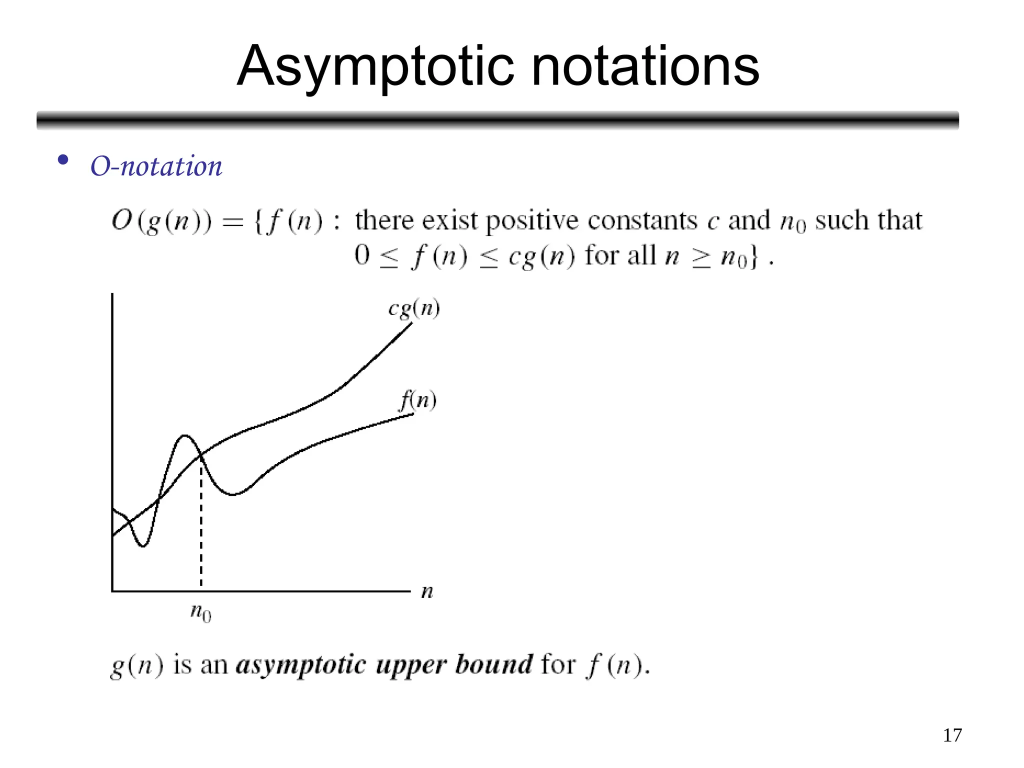
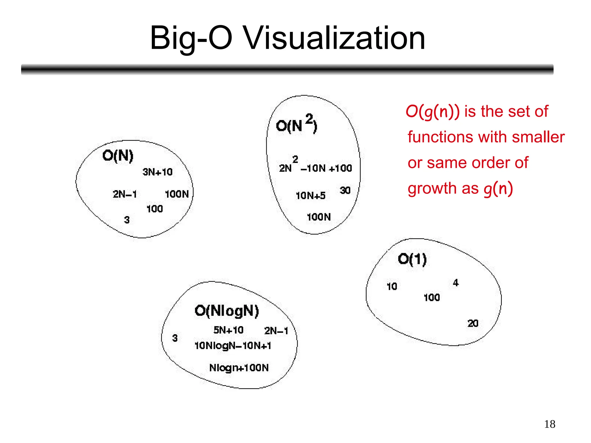
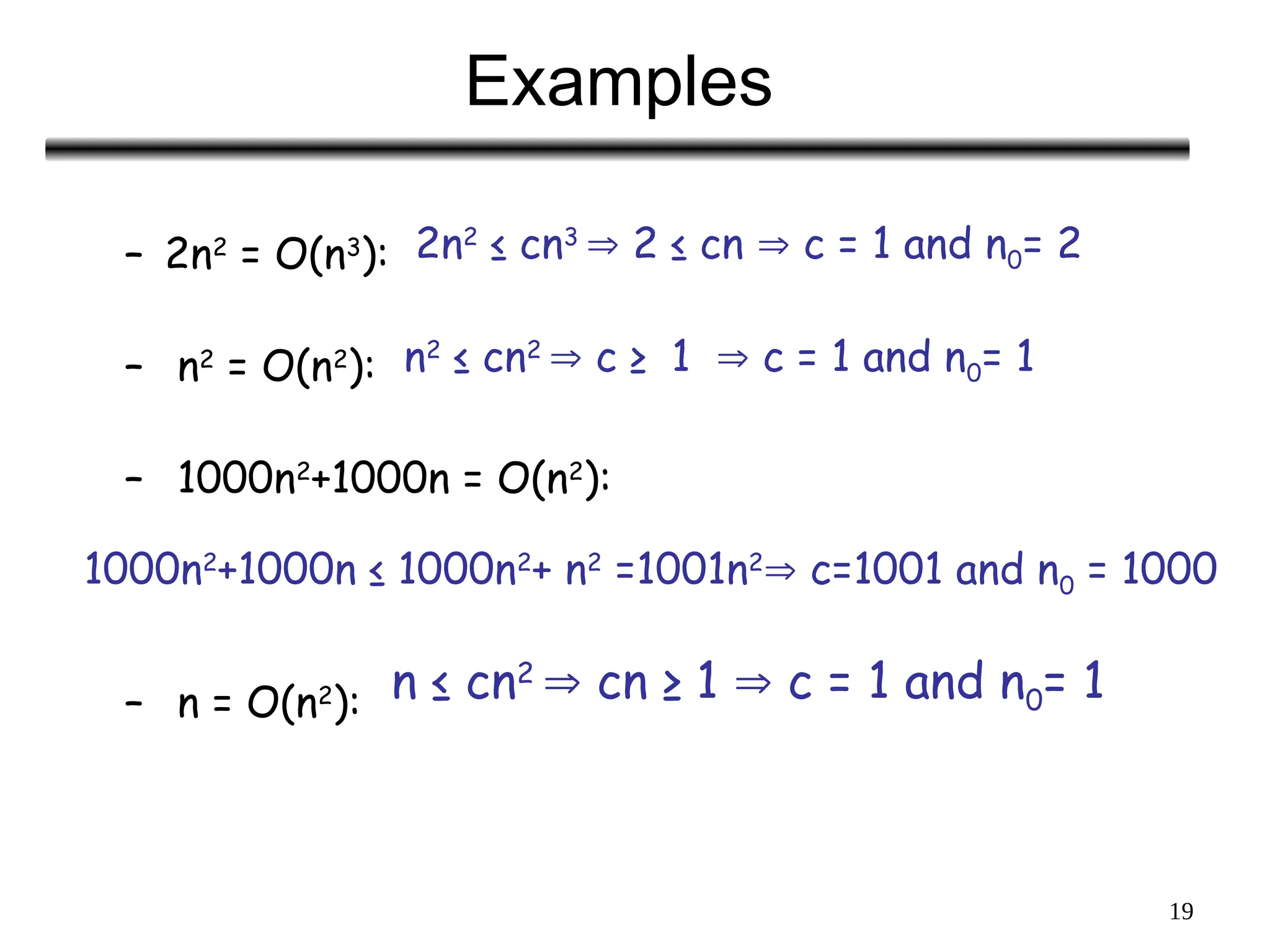
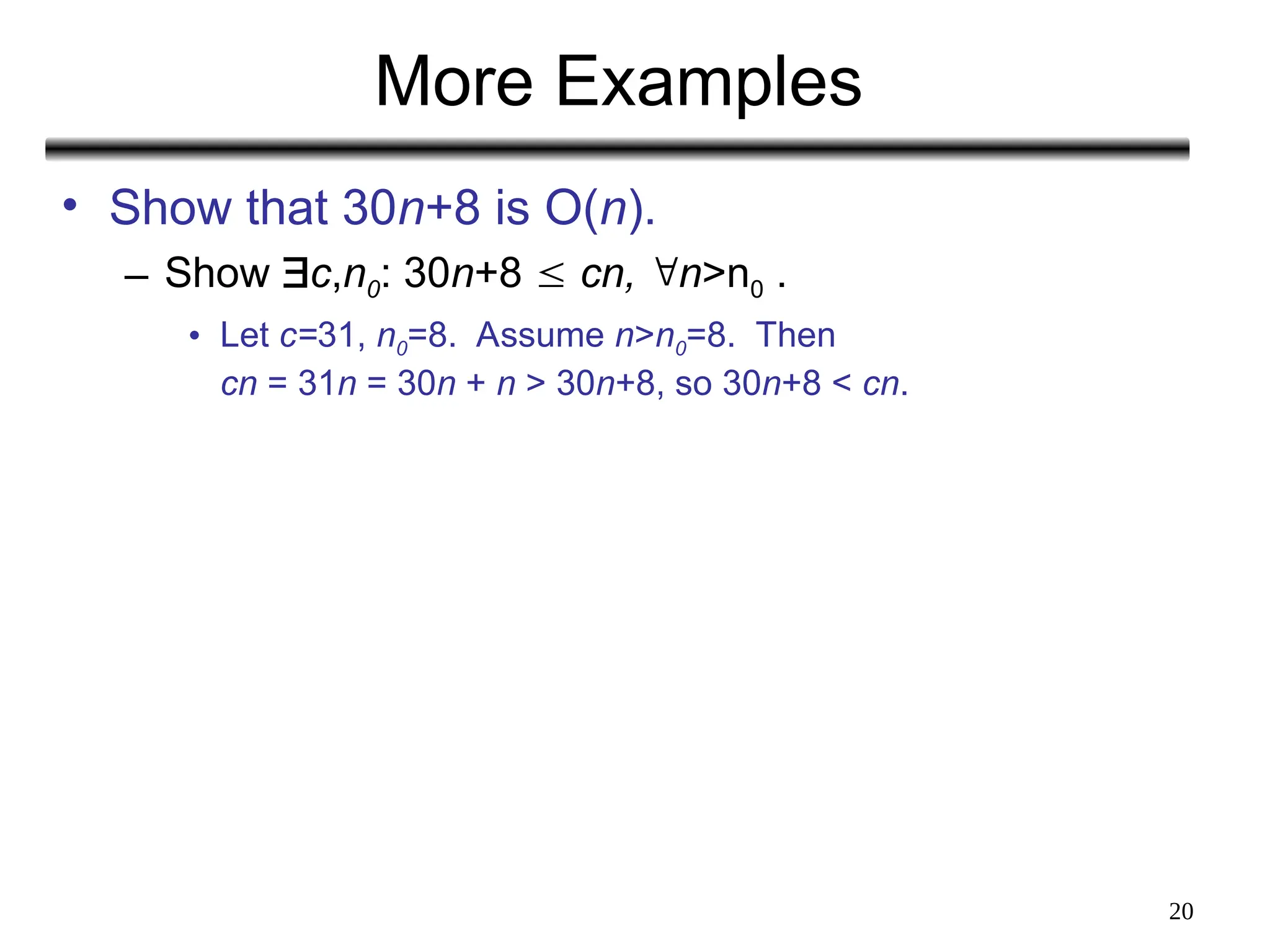
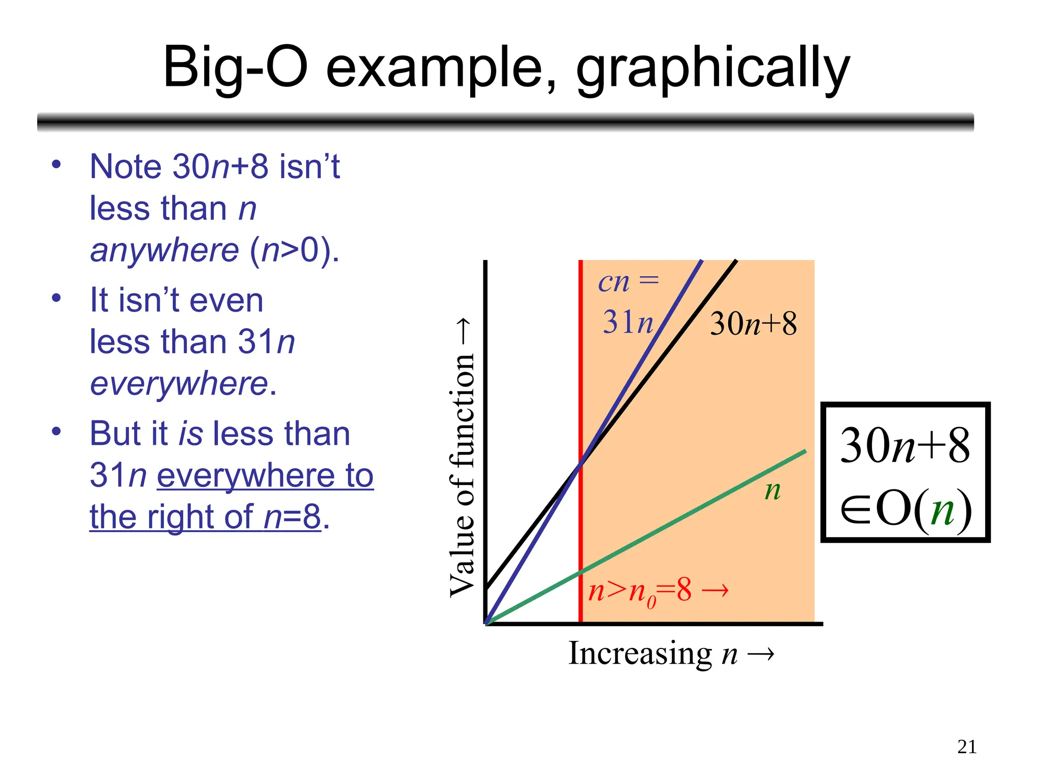
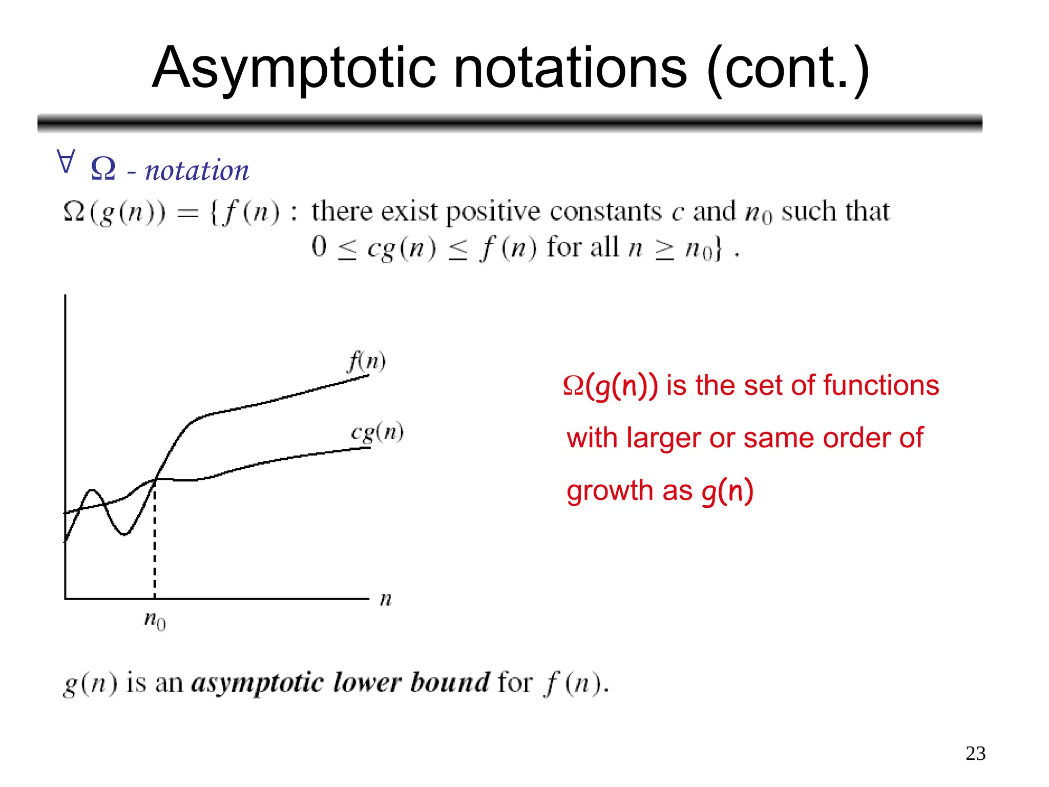
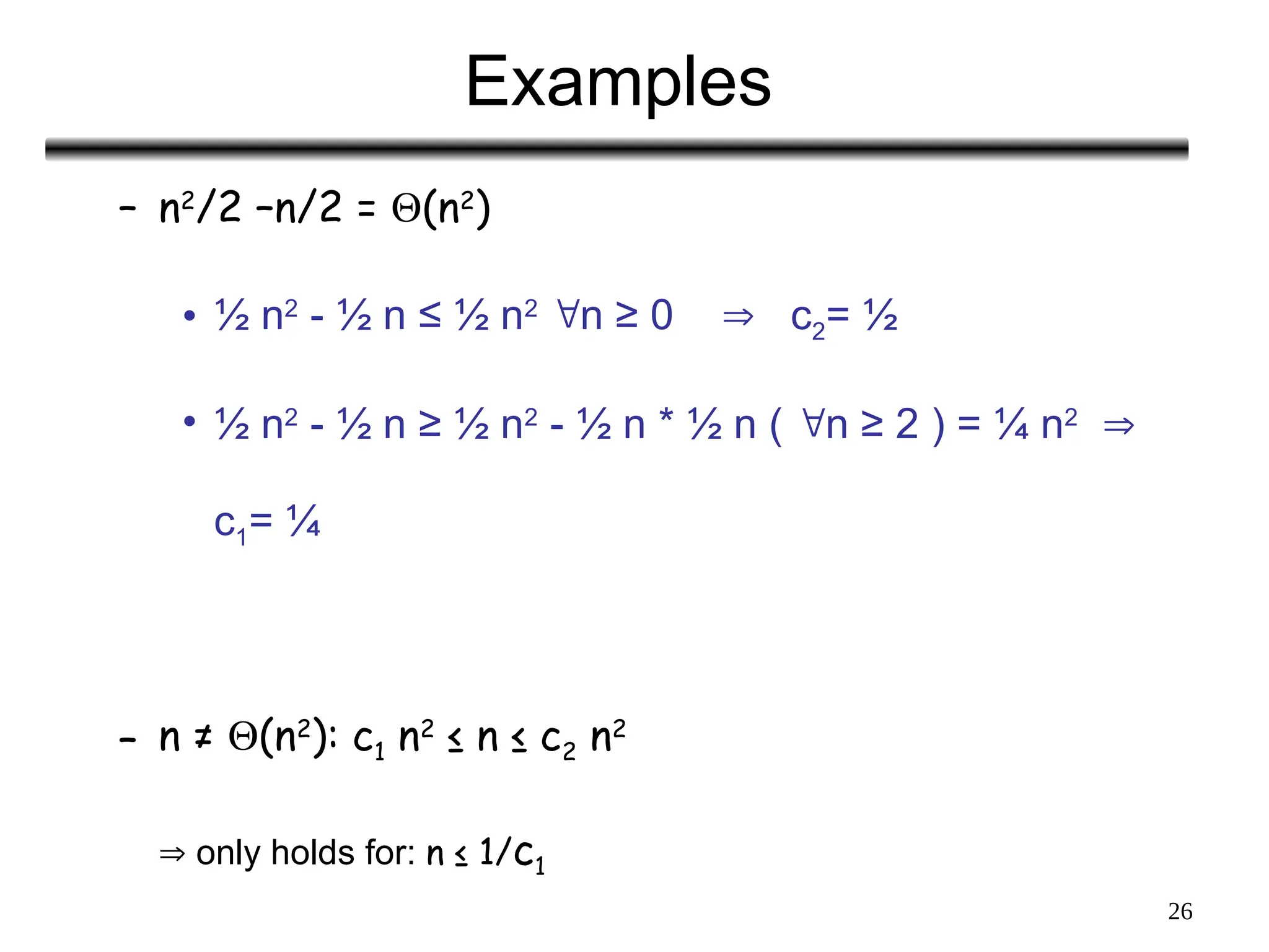
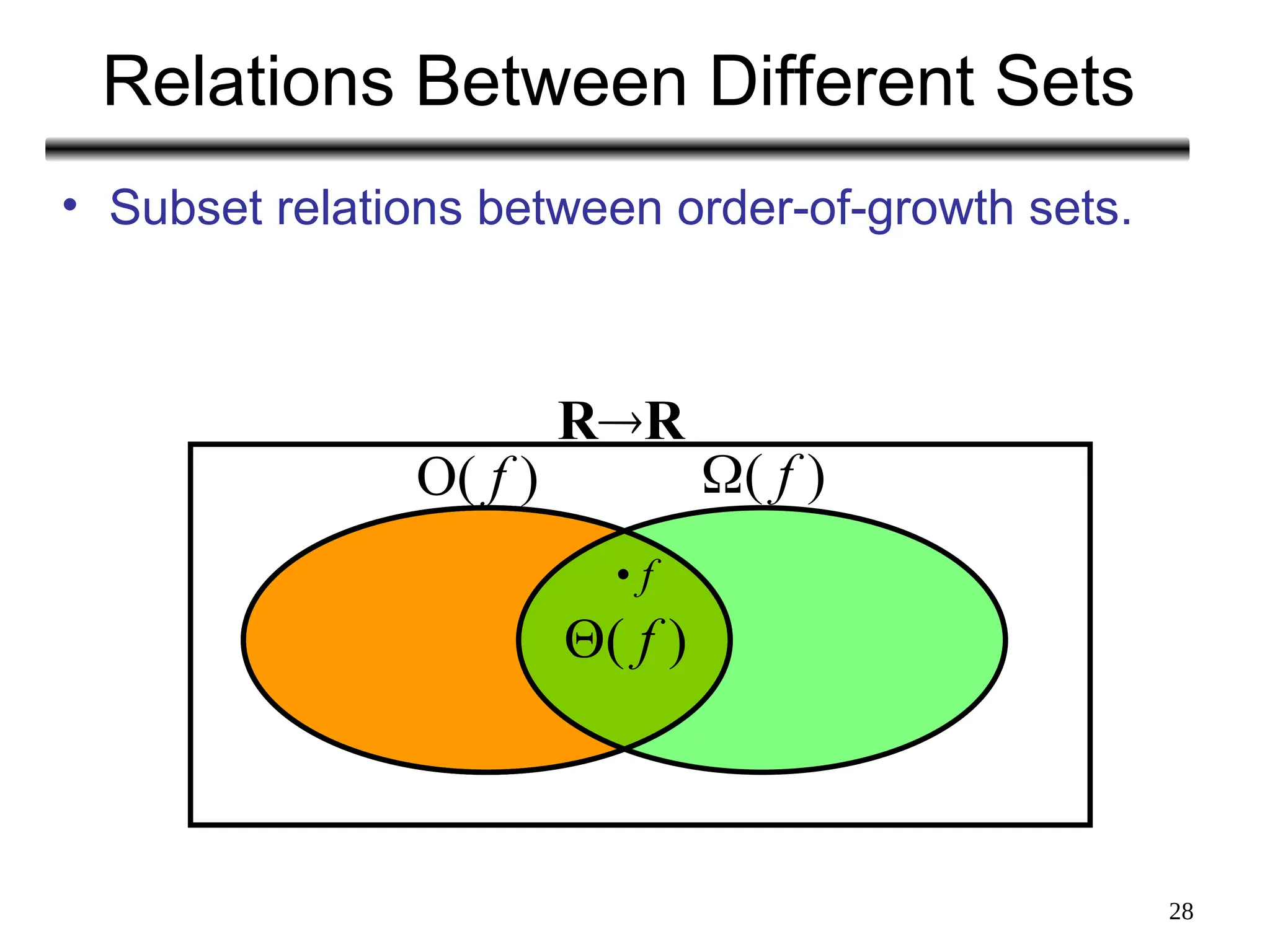
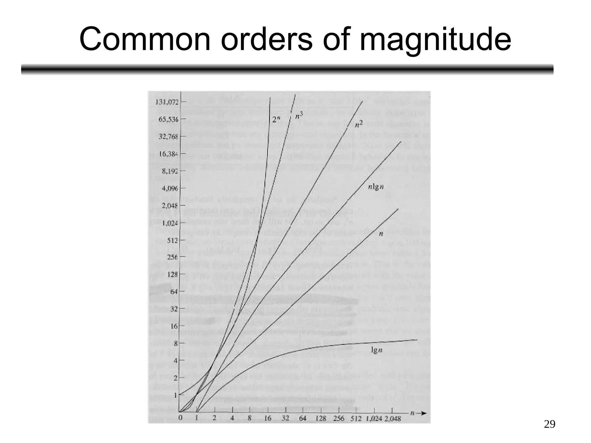
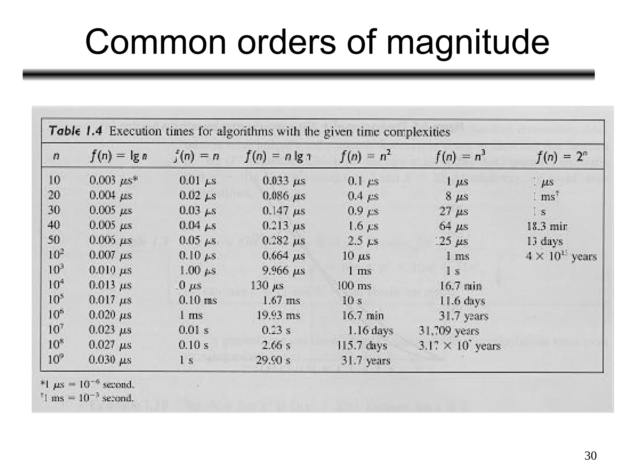
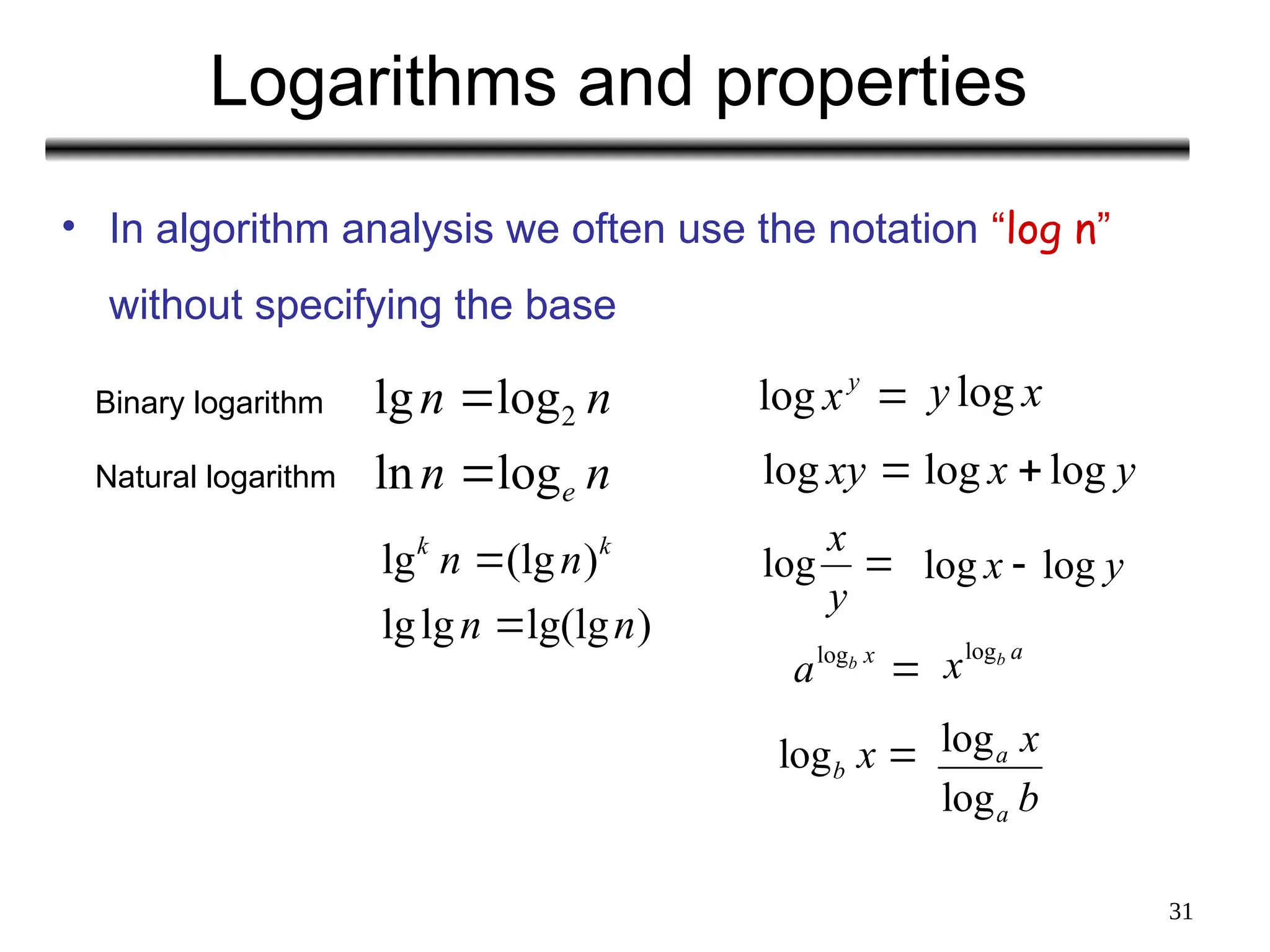
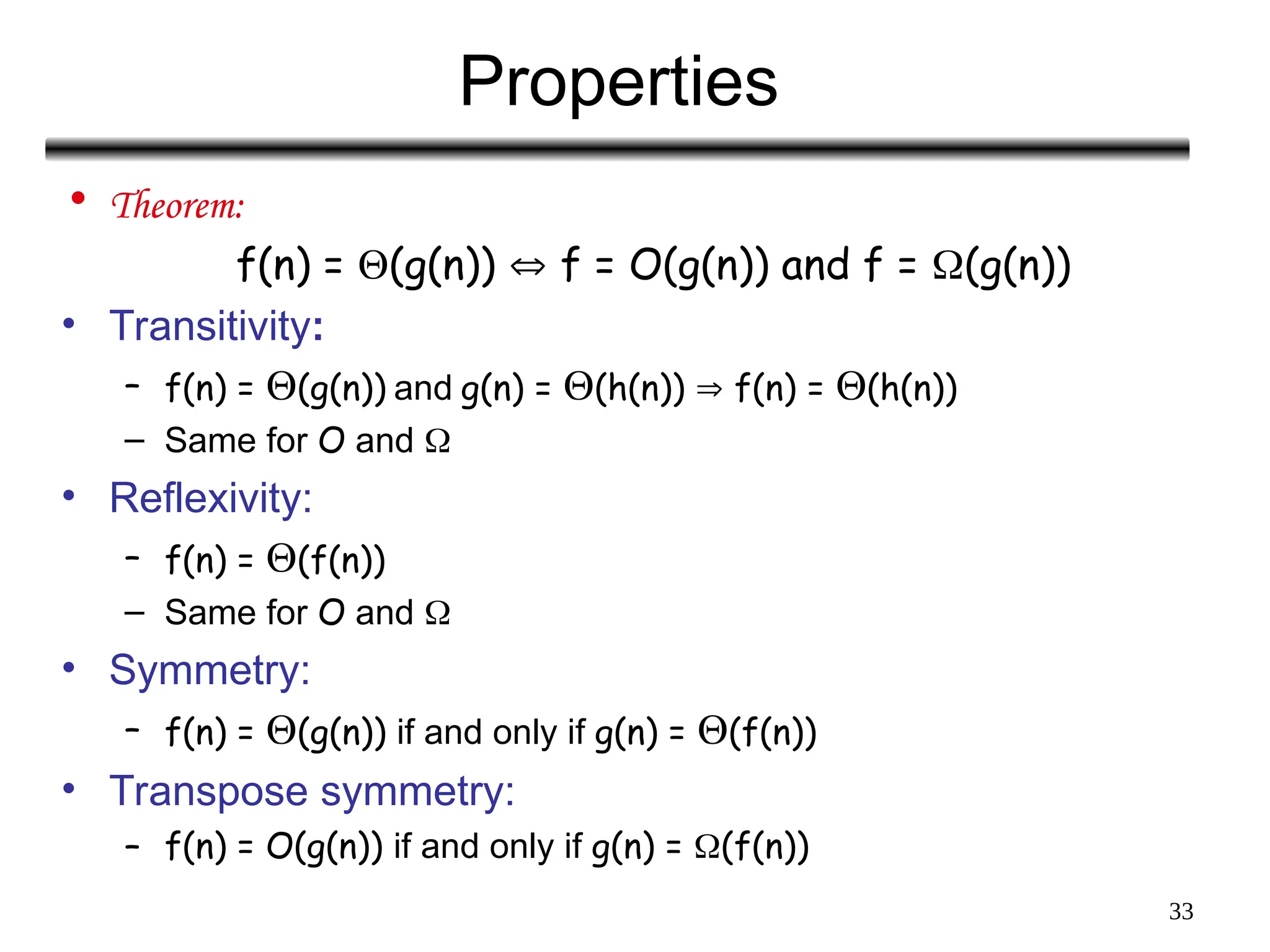
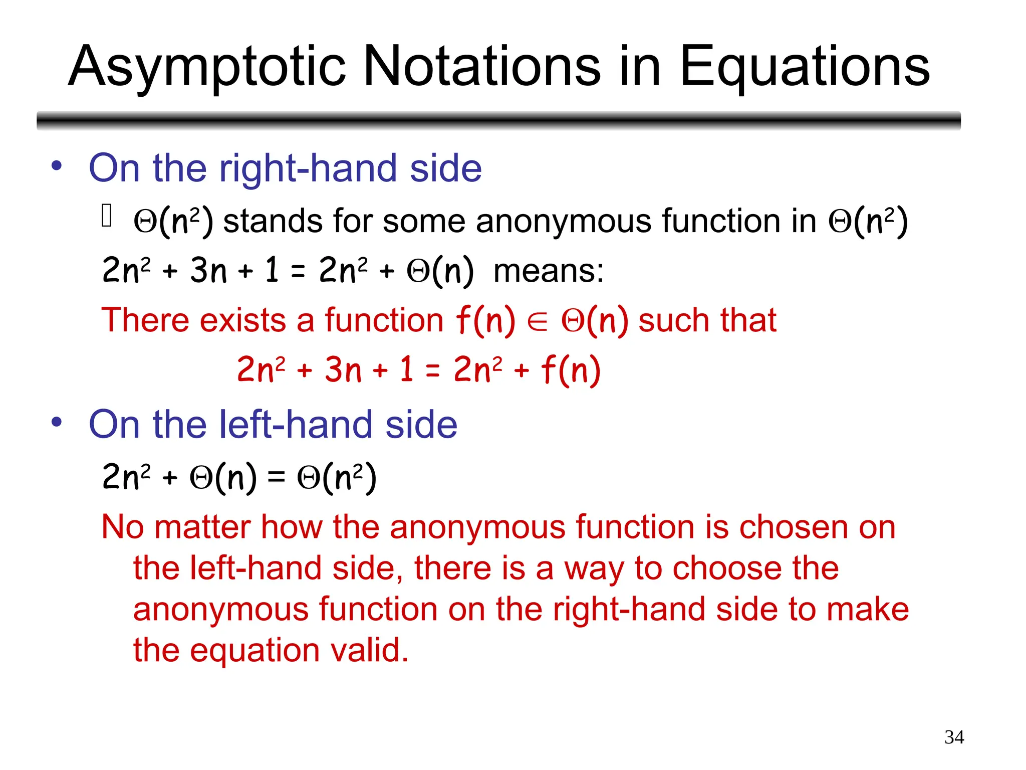
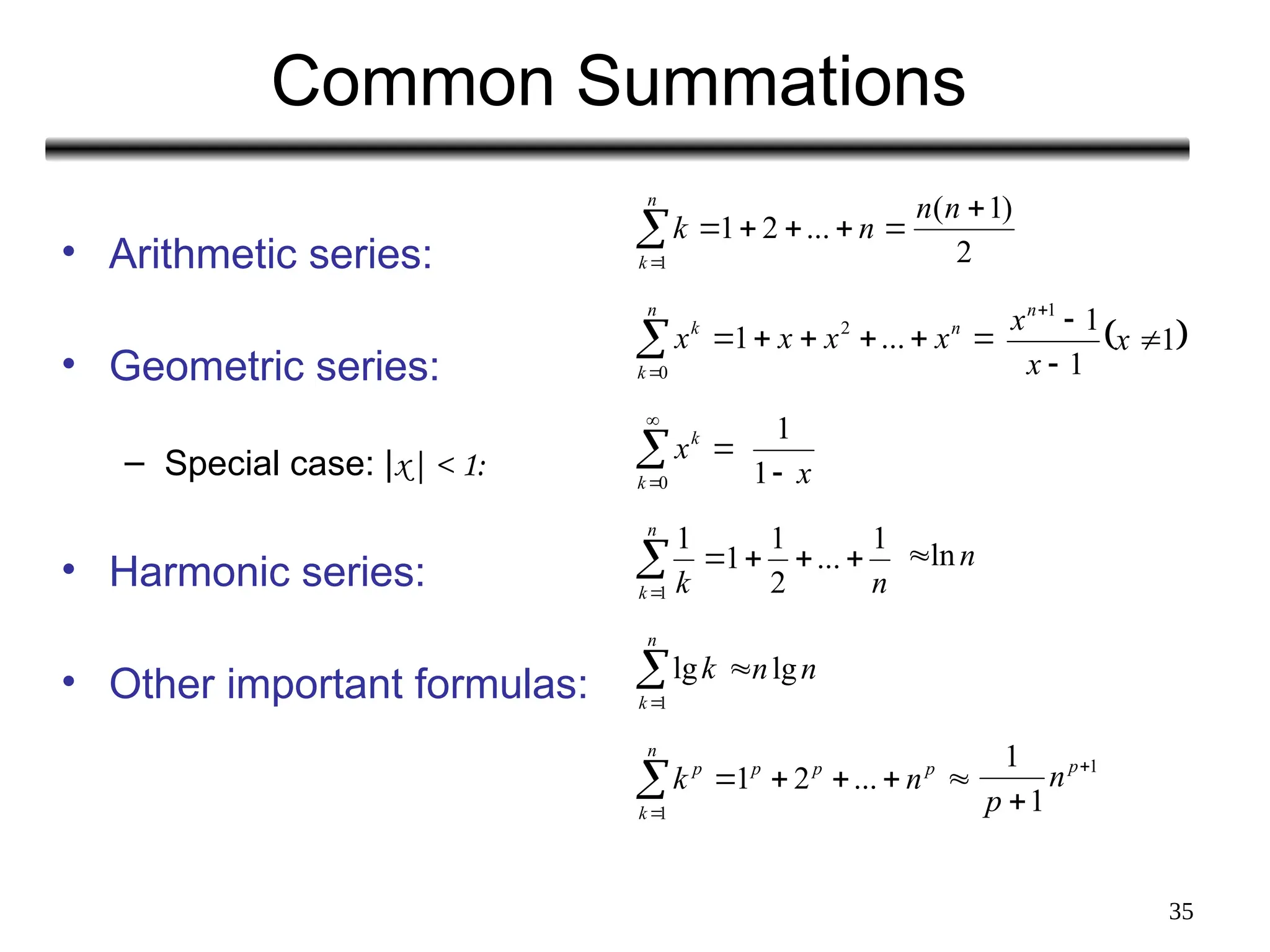
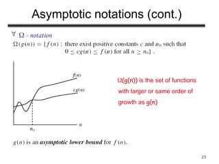
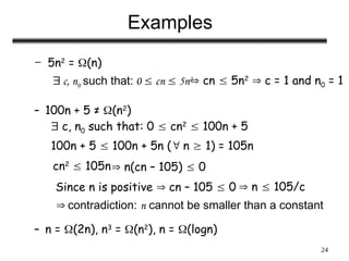
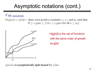
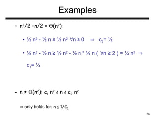
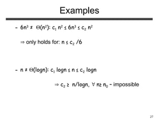
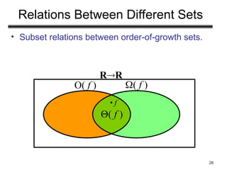
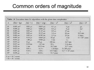
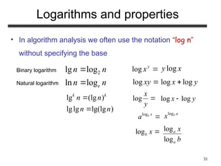
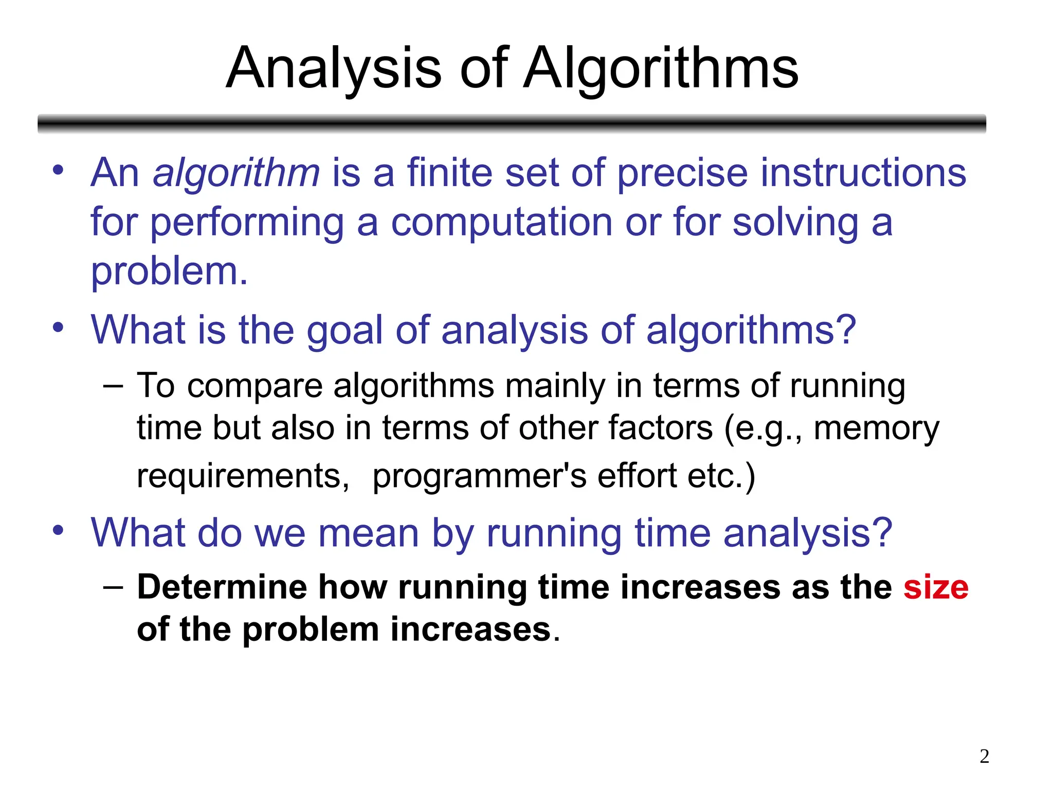
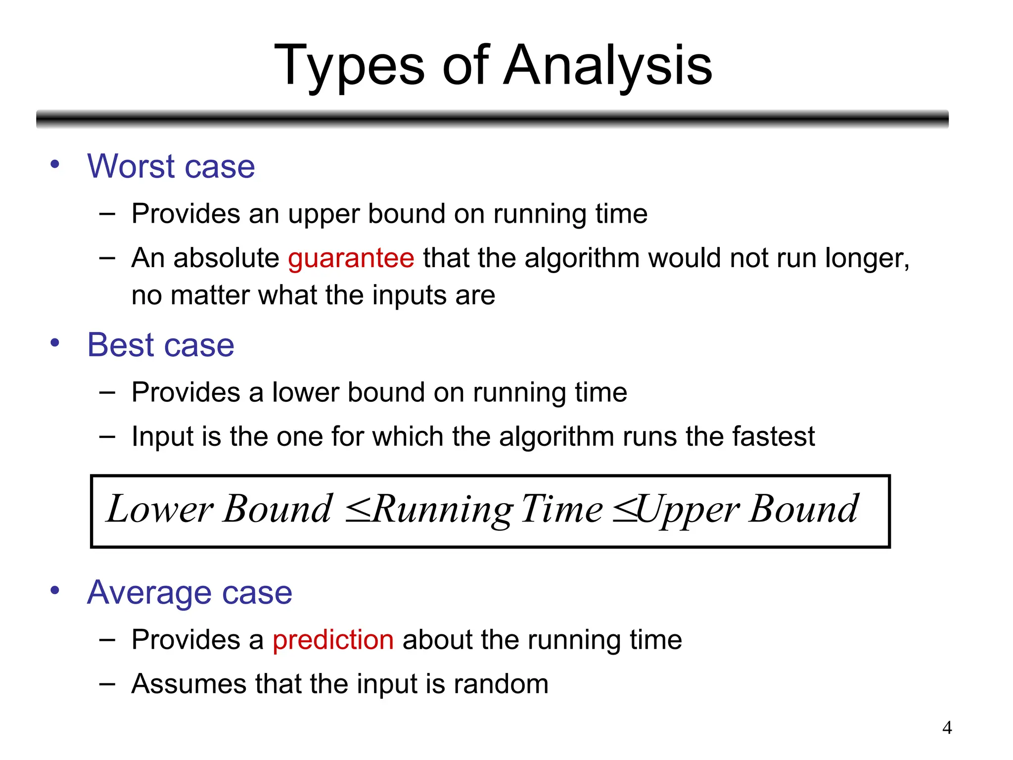
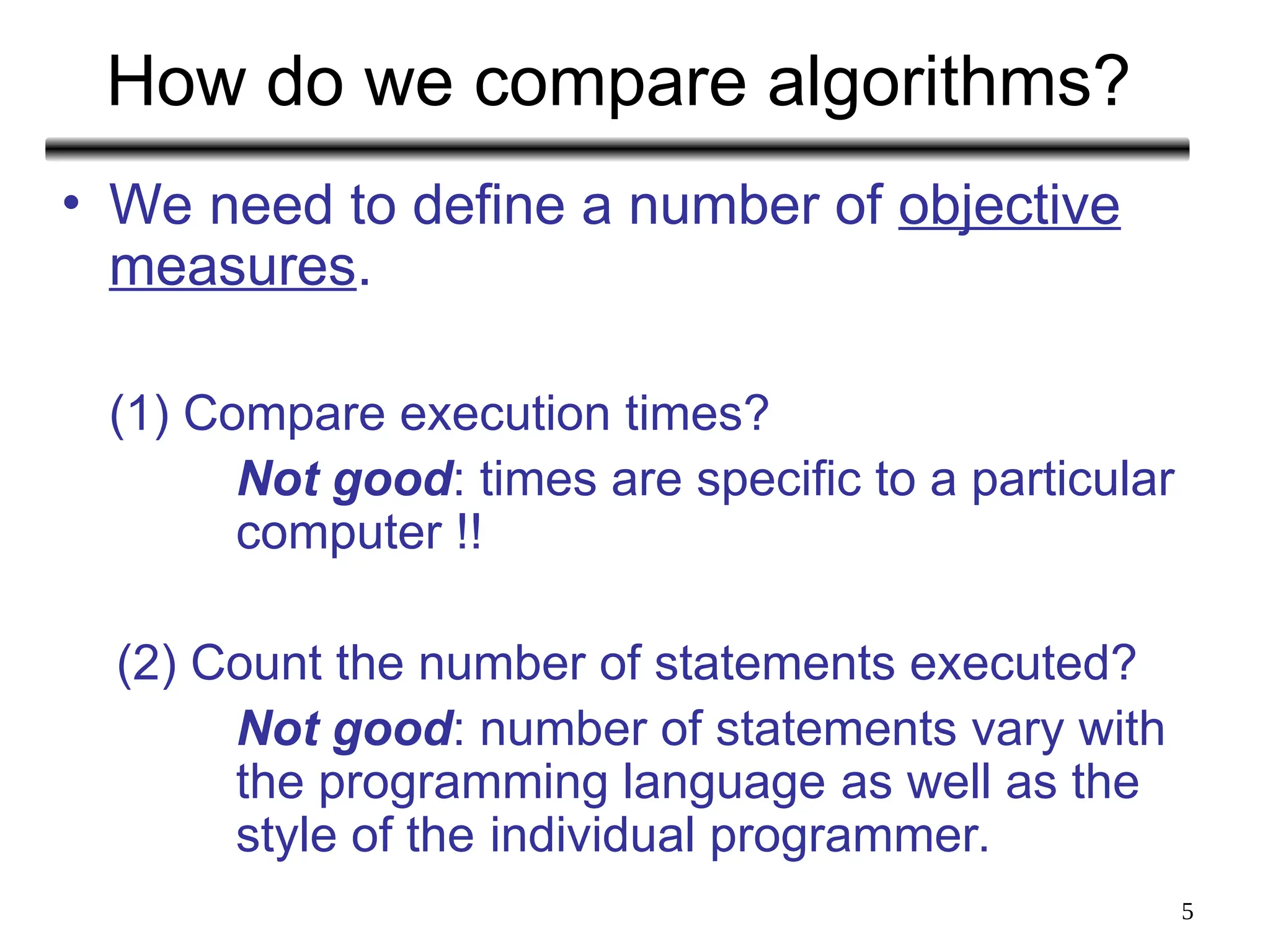
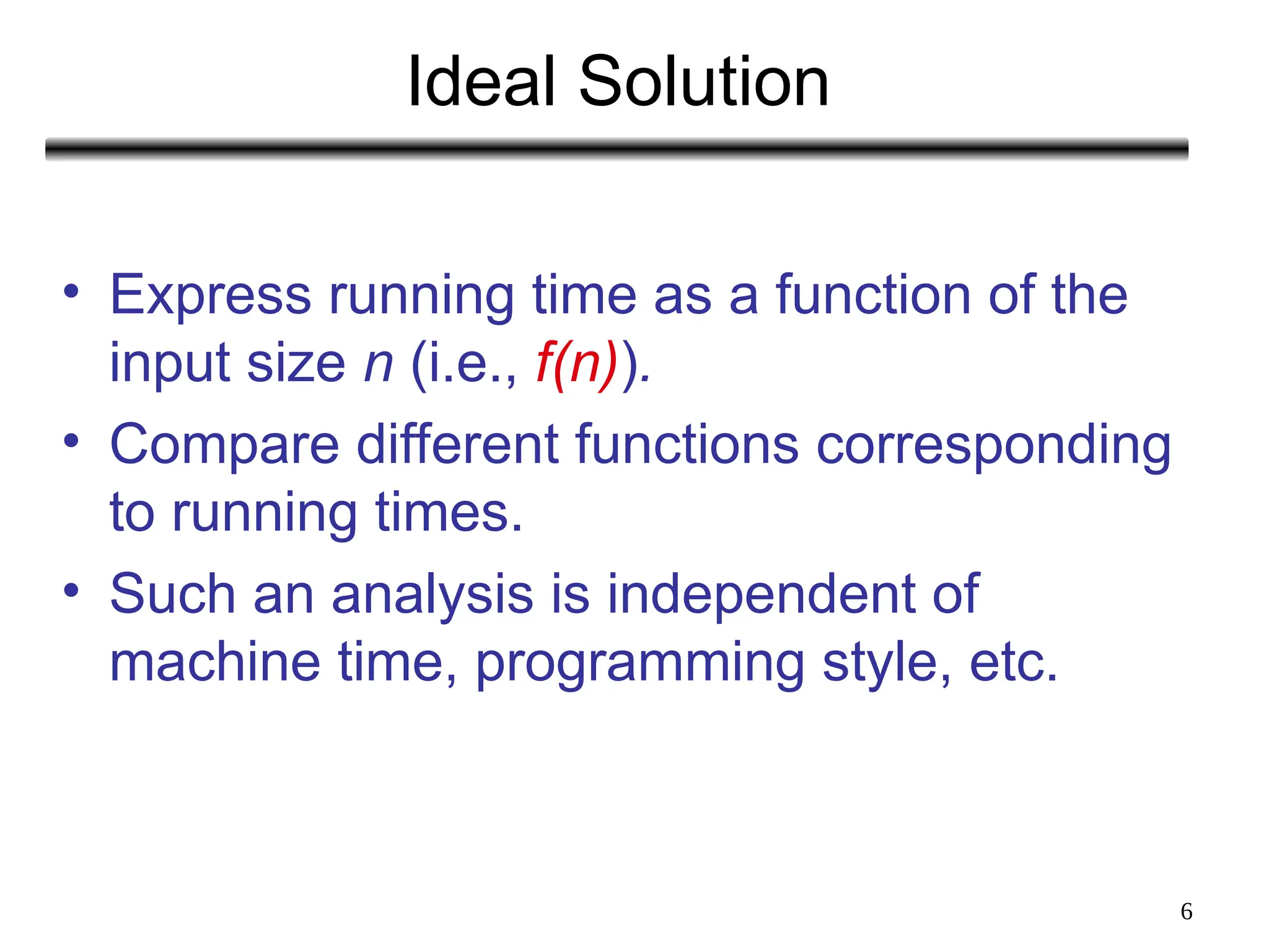
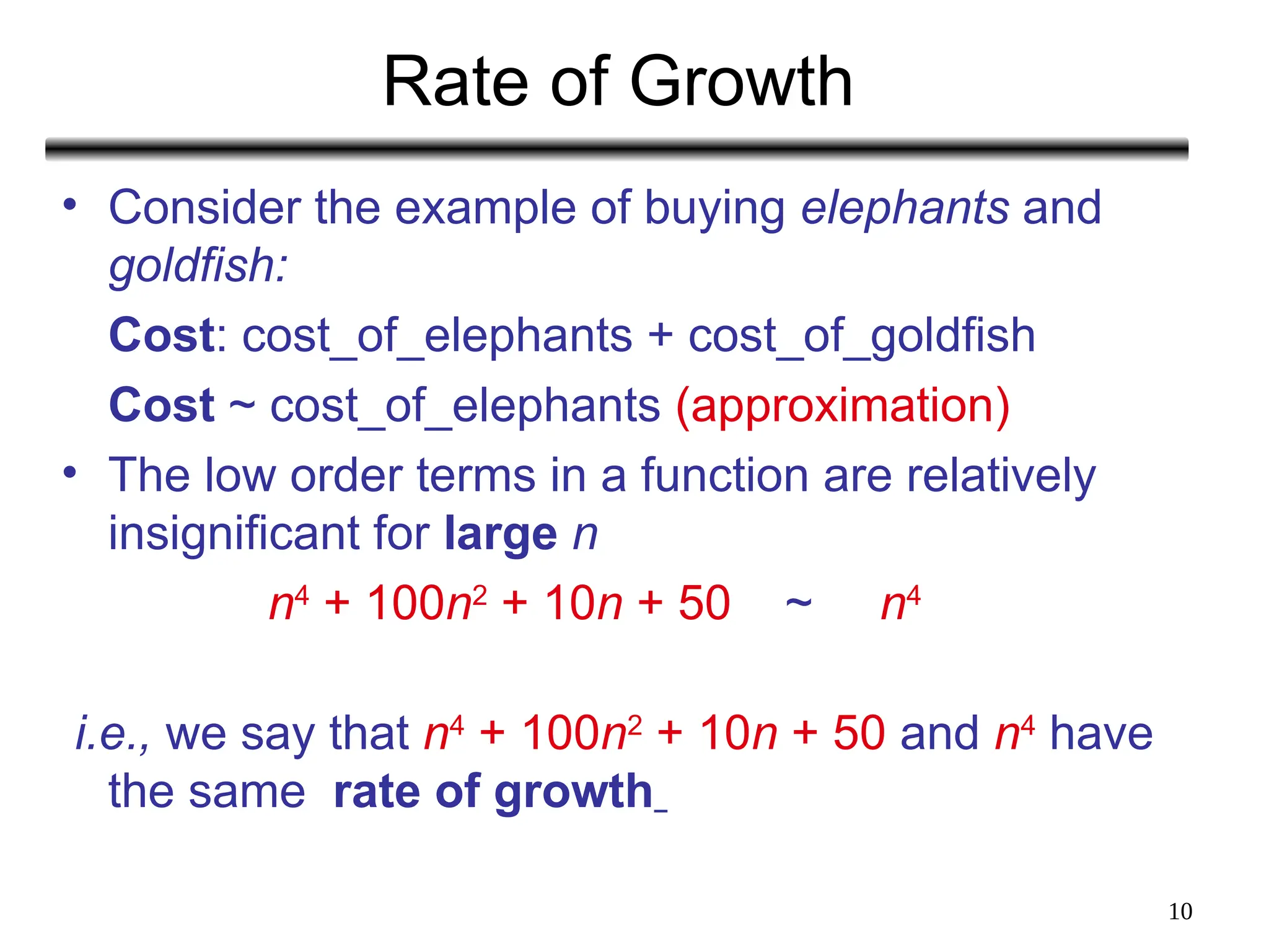
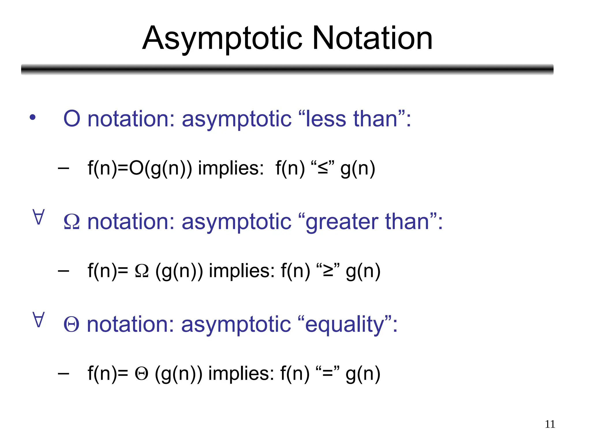
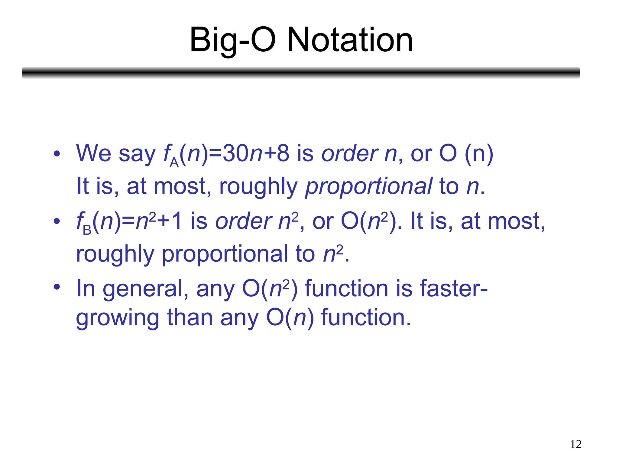
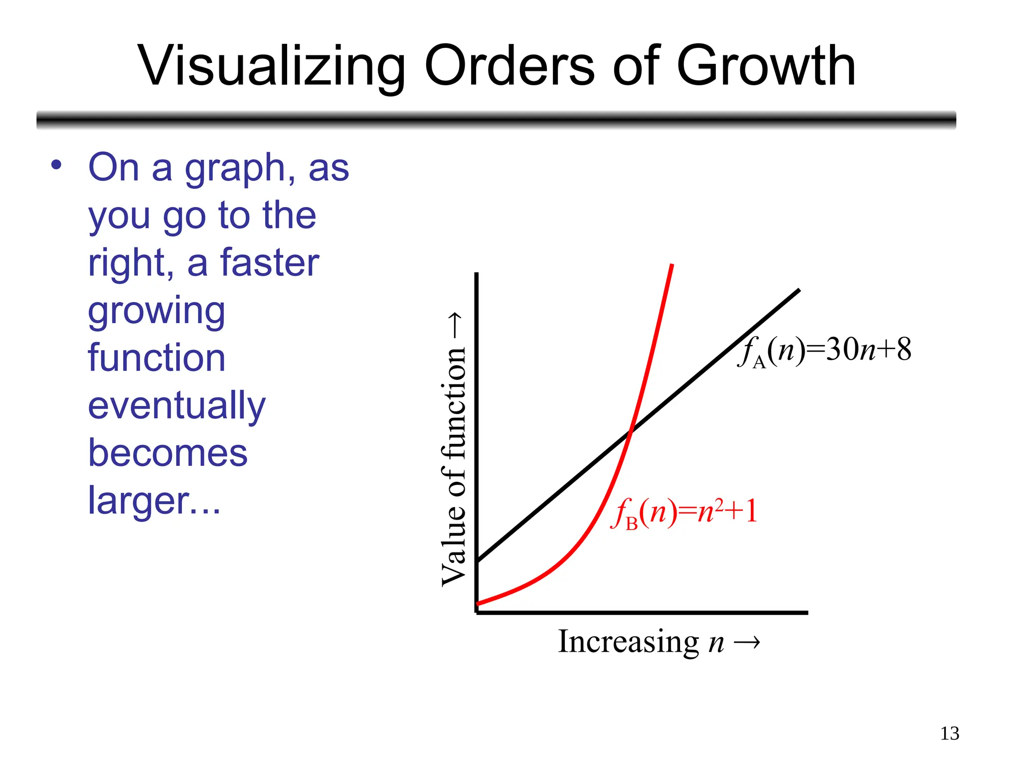
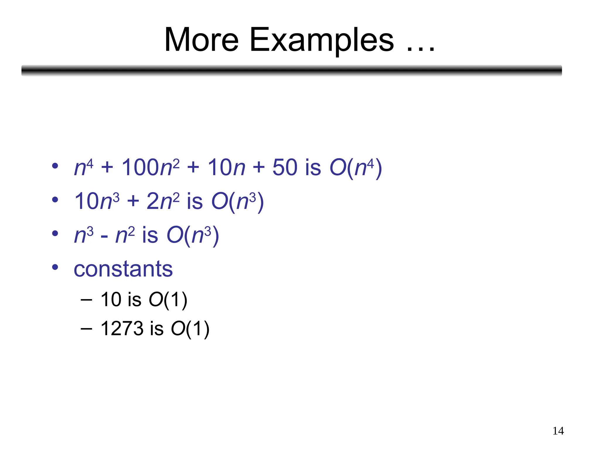
The document discusses the analysis of algorithms, focusing on asymptotic analysis to compare running times of algorithms based on their input size and growth rates. It introduces various types of analysis such as worst case, best case, and average case, as well as asymptotic notations (o, Ω, Θ, and Big-O) for characterizing the growth of functions. The document provides examples and illustrations of how to use these concepts to determine the efficiency of algorithms regardless of programming language or hardware specifics.

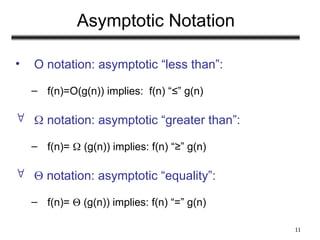
![7
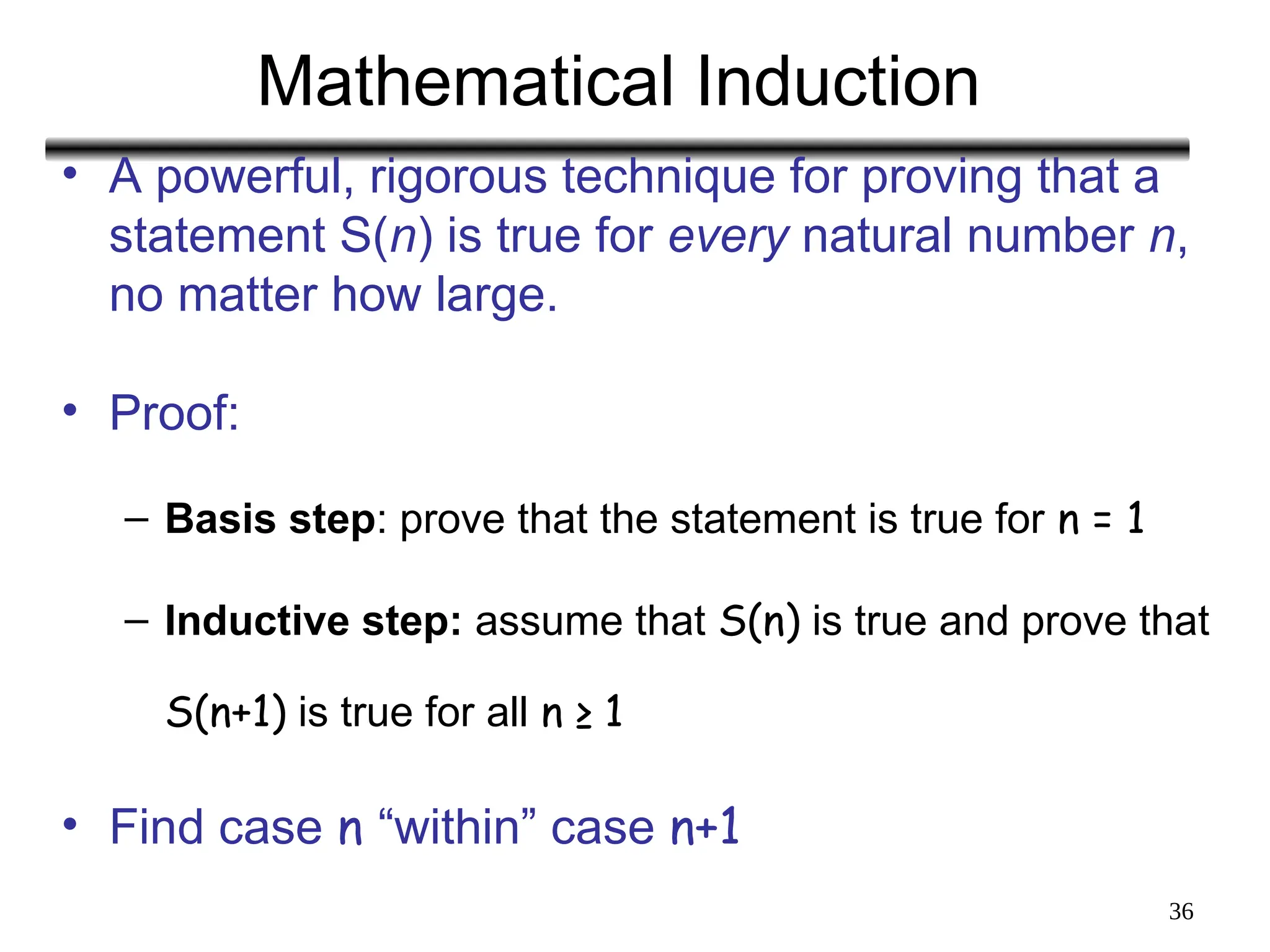
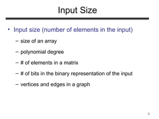
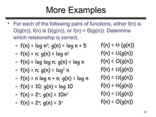
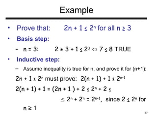
Example
• Associate a "cost" with each statement.
• Find the "total cost“ by finding the total number of times
each statement is executed.
Algorithm 1 Algorithm 2
Cost Cost
arr[0] = 0; c1 for(i=0; i<N; i++) c2
arr[1] = 0; c1 arr[i] = 0; c1
arr[2] = 0; c1
... ...
arr[N-1] = 0; c1
----------- -------------
c1+c1+...+c1 = c1 x N (N+1) x c2 + N x c1 =
(c2 + c1) x N + c2](https://image.slidesharecdn.com/asymptoticanalysis-240822023531-280c65c2/85/AsymptoticAnalysis-goal-of-analysis-of-algorithms-7-320.jpg)
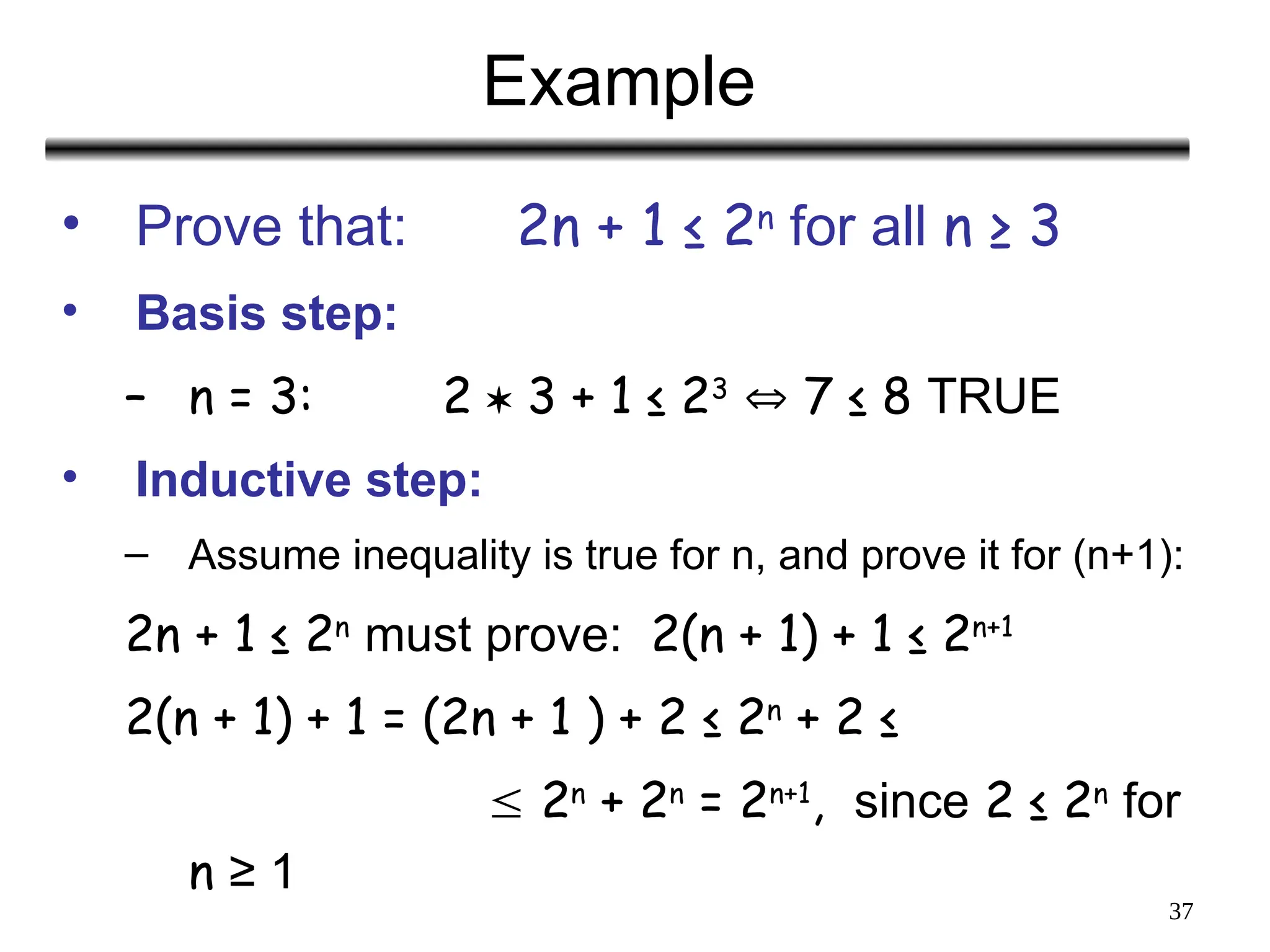
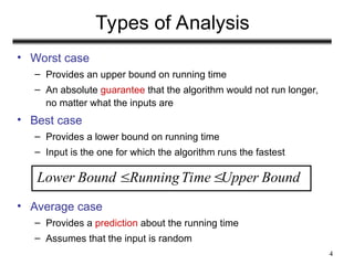
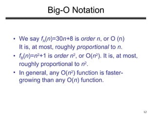
![8
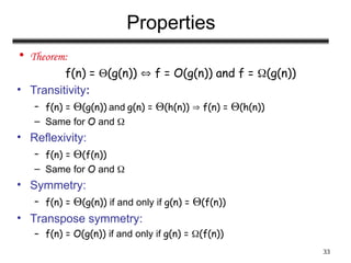
Another Example
• Algorithm 3 Cost
sum = 0; c1
for(i=0; i<N; i++) c2
for(j=0; j<N; j++) c2
sum += arr[i][j]; c3
------------
c1 + c2 x (N+1) + c2 x N x (N+1) + c3 x N2](https://image.slidesharecdn.com/asymptoticanalysis-240822023531-280c65c2/85/AsymptoticAnalysis-goal-of-analysis-of-algorithms-8-320.jpg)


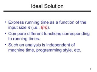
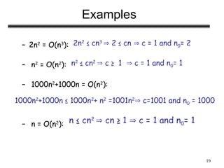
![15
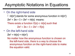
Back to Our Example
Algorithm 1 Algorithm 2
Cost Cost
arr[0] = 0; c1 for(i=0; i<N; i++) c2
arr[1] = 0; c1 arr[i] = 0; c1
arr[2] = 0; c1
...
arr[N-1] = 0; c1
----------- -------------
c1+c1+...+c1 = c1 x N (N+1) x c2 + N x c1 =
(c2 + c1) x N + c2
• Both algorithms are of the same order: O(N)](https://image.slidesharecdn.com/asymptoticanalysis-240822023531-280c65c2/85/AsymptoticAnalysis-goal-of-analysis-of-algorithms-15-320.jpg)
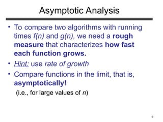
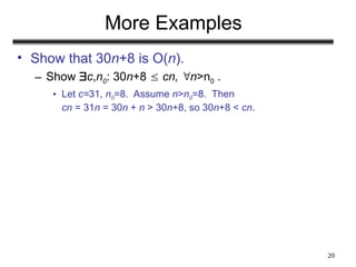
![16
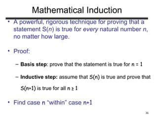
Example (cont’d)
Algorithm 3 Cost
sum = 0; c1
for(i=0; i<N; i++) c2
for(j=0; j<N; j++) c2
sum += arr[i][j]; c3
------------
c1 + c2 x (N+1) + c2 x N x (N+1) + c3 x N2
= O(N2
)](https://image.slidesharecdn.com/asymptoticanalysis-240822023531-280c65c2/85/AsymptoticAnalysis-goal-of-analysis-of-algorithms-16-320.jpg)


![7
Example
• Associate a "cost" with each statement.
• Find the "total cost“ by finding the total number of times
each statement is executed.
Algorithm 1 Algorithm 2
Cost Cost
arr[0] = 0; c1 for(i=0; i<N; i++) c2
arr[1] = 0; c1 arr[i] = 0; c1
arr[2] = 0; c1
... ...
arr[N-1] = 0; c1
----------- -------------
c1+c1+...+c1 = c1 x N (N+1) x c2 + N x c1 =
(c2 + c1) x N + c2](https://image.slidesharecdn.com/asymptoticanalysis-240822023531-280c65c2/75/AsymptoticAnalysis-goal-of-analysis-of-algorithms-7-2048.jpg)
![8
Another Example
• Algorithm 3 Cost
sum = 0; c1
for(i=0; i<N; i++) c2
for(j=0; j<N; j++) c2
sum += arr[i][j]; c3
------------
c1 + c2 x (N+1) + c2 x N x (N+1) + c3 x N2](https://image.slidesharecdn.com/asymptoticanalysis-240822023531-280c65c2/75/AsymptoticAnalysis-goal-of-analysis-of-algorithms-8-2048.jpg)

![15
Back to Our Example
Algorithm 1 Algorithm 2
Cost Cost
arr[0] = 0; c1 for(i=0; i<N; i++) c2
arr[1] = 0; c1 arr[i] = 0; c1
arr[2] = 0; c1
...
arr[N-1] = 0; c1
----------- -------------
c1+c1+...+c1 = c1 x N (N+1) x c2 + N x c1 =
(c2 + c1) x N + c2
• Both algorithms are of the same order: O(N)](https://image.slidesharecdn.com/asymptoticanalysis-240822023531-280c65c2/75/AsymptoticAnalysis-goal-of-analysis-of-algorithms-15-2048.jpg)
![16
Example (cont’d)
Algorithm 3 Cost
sum = 0; c1
for(i=0; i<N; i++) c2
for(j=0; j<N; j++) c2
sum += arr[i][j]; c3
------------
c1 + c2 x (N+1) + c2 x N x (N+1) + c3 x N2
= O(N2
)](https://image.slidesharecdn.com/asymptoticanalysis-240822023531-280c65c2/75/AsymptoticAnalysis-goal-of-analysis-of-algorithms-16-2048.jpg)