


![MEMOIZATION
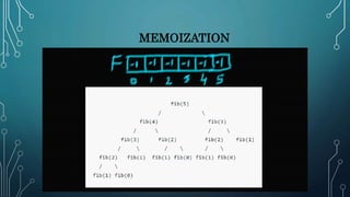
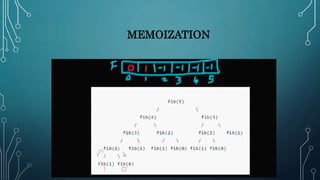
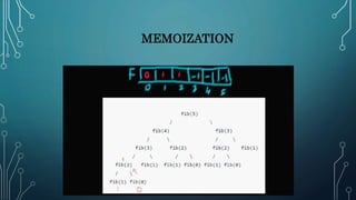
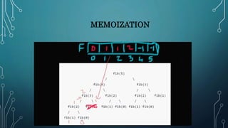
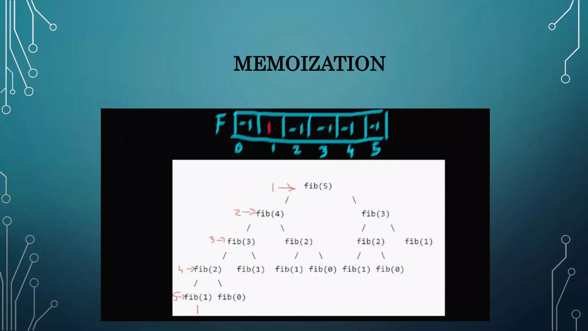
• At every step i, f(i) performs the following steps:
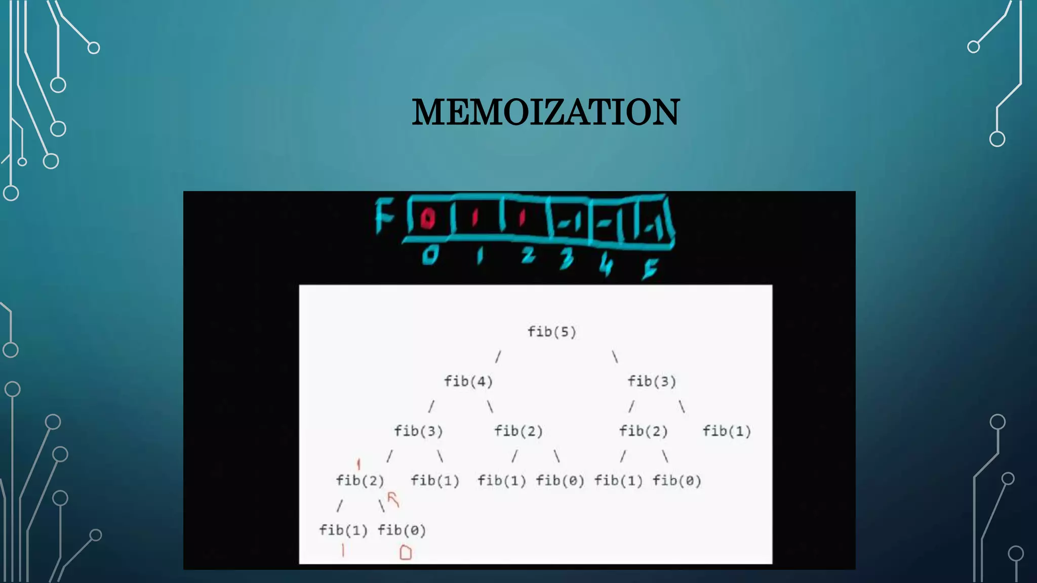
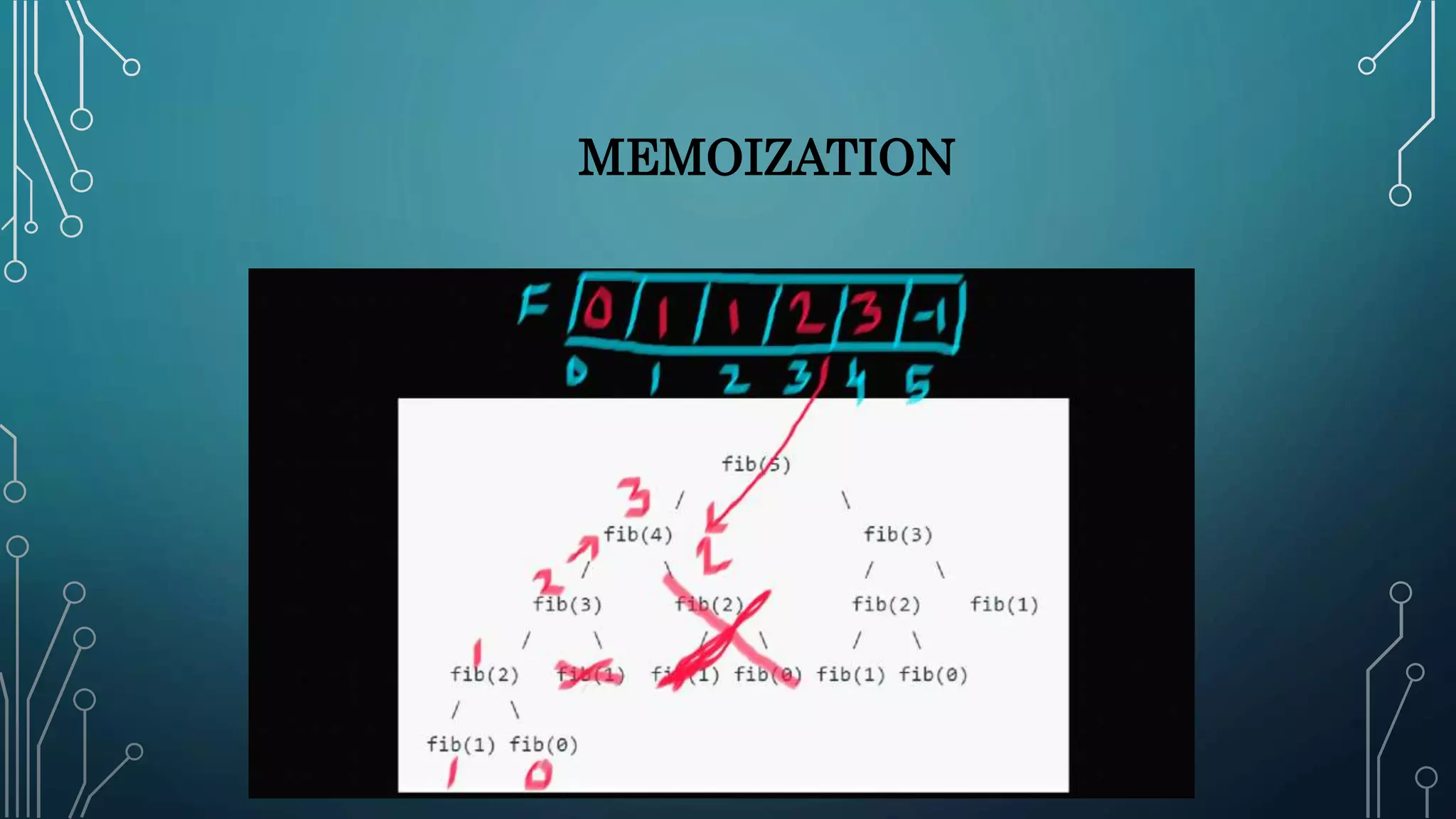
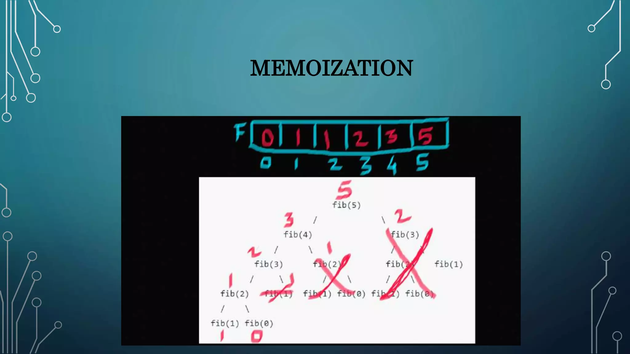
1. Checks whether table[i] is NIL or not.
2. If it’s not NIL, f(i) returns the value ‘table[i]’.
3. If it’s NIL and ‘i’ satisfies the base condition, we update the lookup table with
the base value and return the same.
4. If it’s NIL and ‘i’ does not satisfy the base condition, then f(i) splits the
problem ‘i’ into subproblems and recursively calls itself to solve them.
5. After the recursive calls return, f(i) combines the solution to subproblems,
update the lookup table and returns the solution for problem ‘i’.](https://image.slidesharecdn.com/vishwajeetelementofdynamicprogrammingaat-210625122607/85/Elements-of-Dynamic-Programming-9-320.jpg)


![TABULATION
• STEPS
a. We begin with initializing the base values of ‘i’.
b. Next, we run a loop that iterates over the remaining
c. At every iteration i, f(n) updates the ith entry in the
by combining the solutions to previously solved
d. Finally, f(n) returns table[n].](https://image.slidesharecdn.com/vishwajeetelementofdynamicprogrammingaat-210625122607/85/Elements-of-Dynamic-Programming-17-320.jpg)
![TABULATION
int fib(int n){
if(n <= 1)
return n;
f[0] = 0; f[1] = 1;
for(int i = 2; I <= n; i++){
f[i] = f[i-2] + f[i-1];
}
return n;
}](https://image.slidesharecdn.com/vishwajeetelementofdynamicprogrammingaat-210625122607/85/Elements-of-Dynamic-Programming-18-320.jpg)


![MEMOIZATION
• At every step i, f(i) performs the following steps:
1. Checks whether table[i] is NIL or not.
2. If it’s not NIL, f(i) returns the value ‘table[i]’.
3. If it’s NIL and ‘i’ satisfies the base condition, we update the lookup table with
the base value and return the same.
4. If it’s NIL and ‘i’ does not satisfy the base condition, then f(i) splits the
problem ‘i’ into subproblems and recursively calls itself to solve them.
5. After the recursive calls return, f(i) combines the solution to subproblems,
update the lookup table and returns the solution for problem ‘i’.](https://image.slidesharecdn.com/vishwajeetelementofdynamicprogrammingaat-210625122607/75/Elements-of-Dynamic-Programming-9-2048.jpg)


![TABULATION
• STEPS
a. We begin with initializing the base values of ‘i’.
b. Next, we run a loop that iterates over the remaining
c. At every iteration i, f(n) updates the ith entry in the
by combining the solutions to previously solved
d. Finally, f(n) returns table[n].](https://image.slidesharecdn.com/vishwajeetelementofdynamicprogrammingaat-210625122607/75/Elements-of-Dynamic-Programming-17-2048.jpg)
![TABULATION
int fib(int n){
if(n <= 1)
return n;
f[0] = 0; f[1] = 1;
for(int i = 2; I <= n; i++){
f[i] = f[i-2] + f[i-1];
}
return n;
}](https://image.slidesharecdn.com/vishwajeetelementofdynamicprogrammingaat-210625122607/75/Elements-of-Dynamic-Programming-18-2048.jpg)


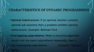
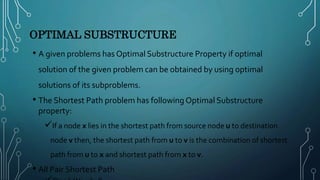
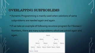
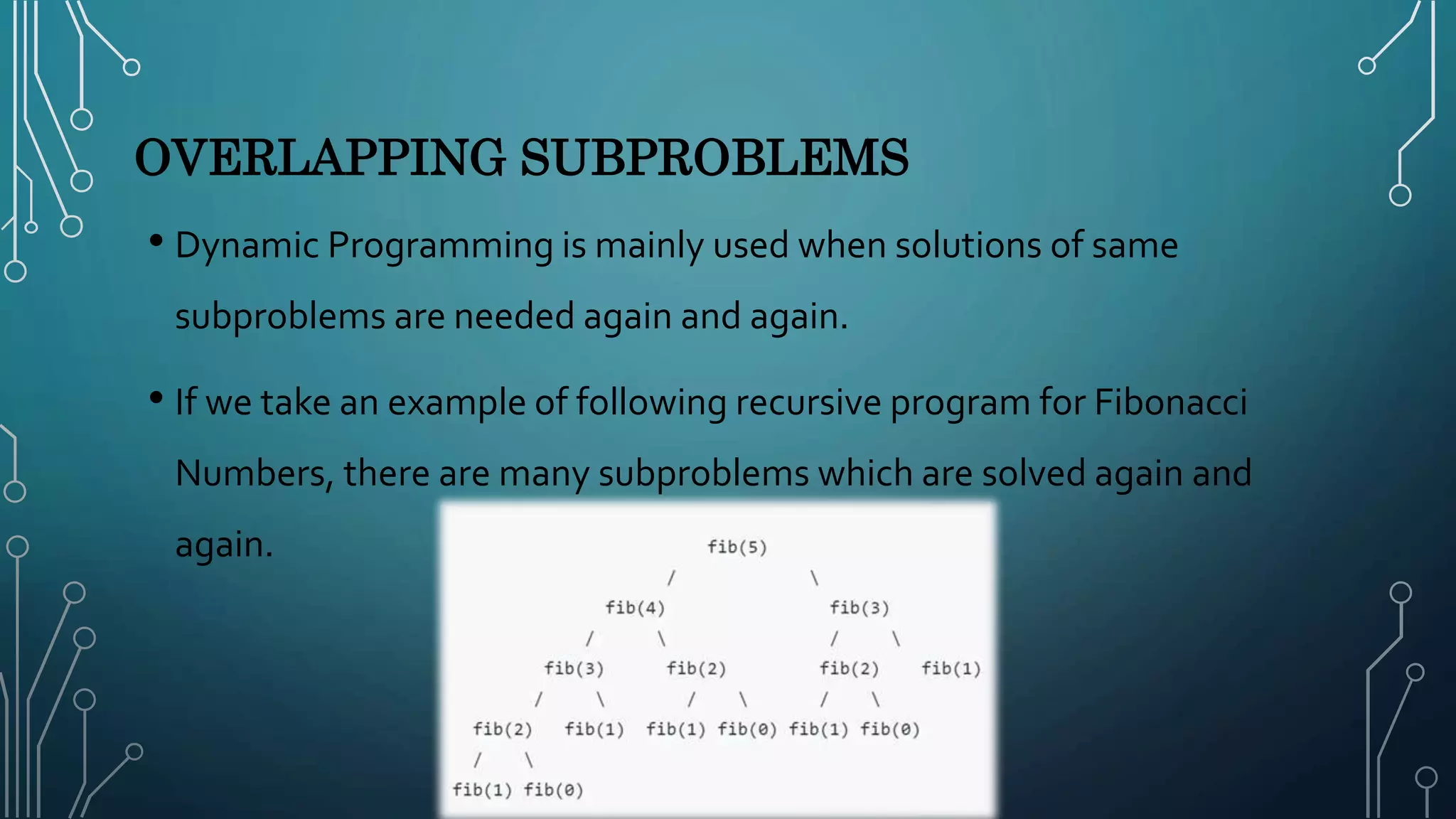
The document presents an overview of dynamic programming, highlighting its significance in solving optimization problems through a bottom-up approach. Key characteristics include optimal substructure and overlapping subproblems, illustrated with examples like the Fibonacci series and shortest path problems. It also explains techniques for storing results in memory, specifically memoization and tabulation, along with performance comparisons in calculating Fibonacci numbers.
Introduction to dynamic programming as a powerful technique for optimization, discussing its bottom-up approach.
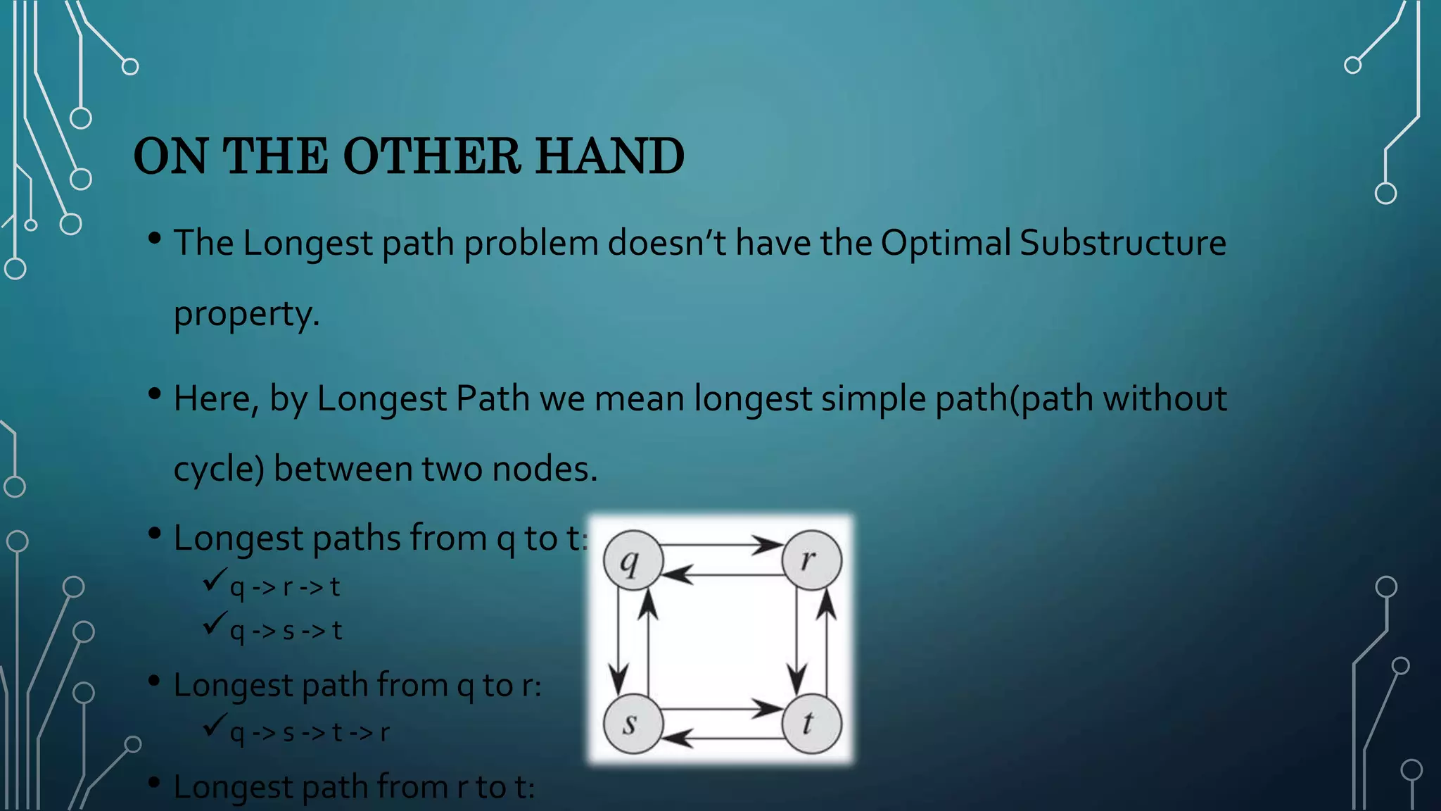
Description of optimal substructure and overlapping subproblems with examples like Bellman-Ford and Fibonacci.
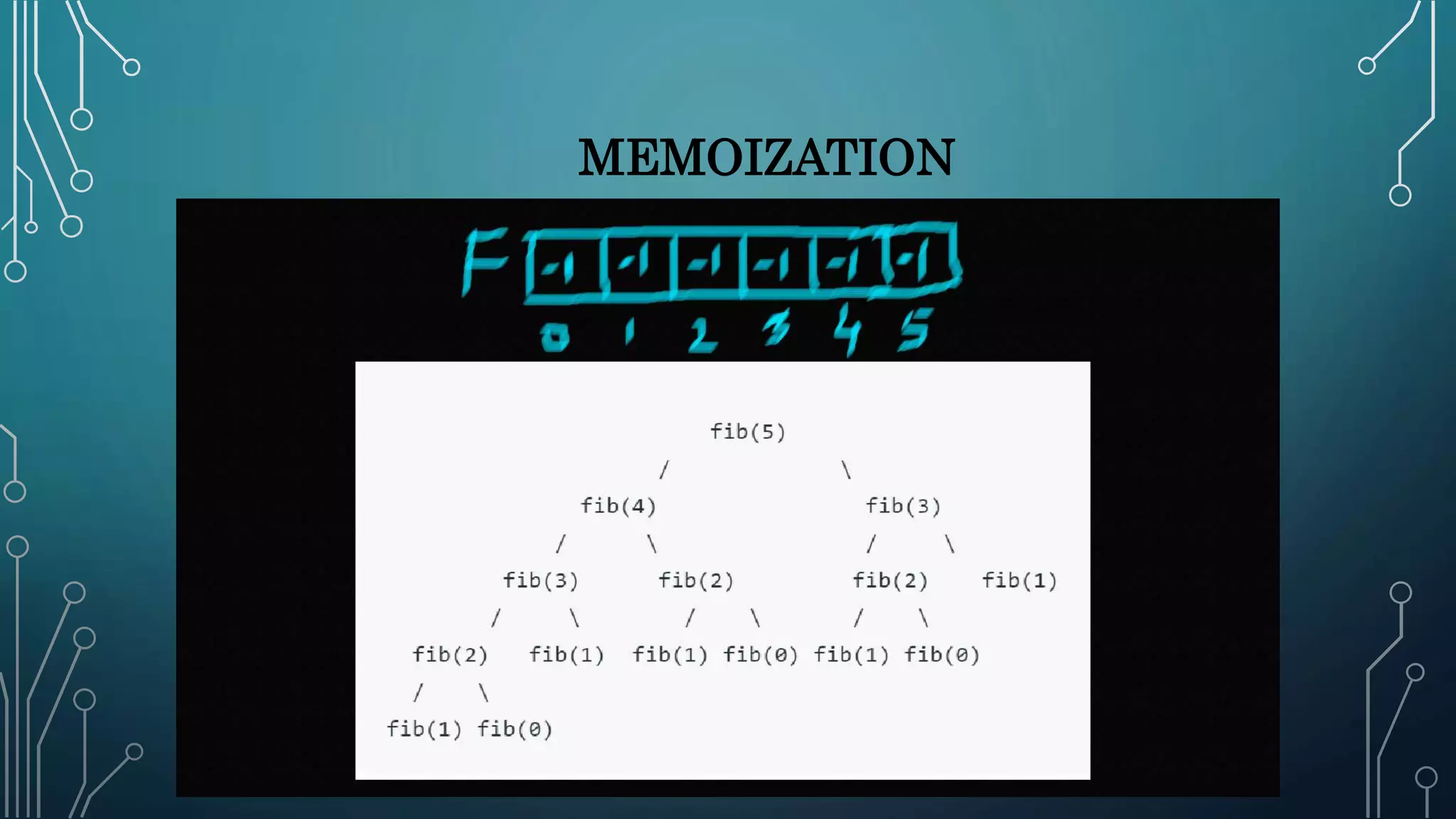
Details on memoization strategy for storing results to avoid repetitive calculations in recursive functions.
Overview of tabulation process in dynamic programming with an example of Fibonacci numbers.
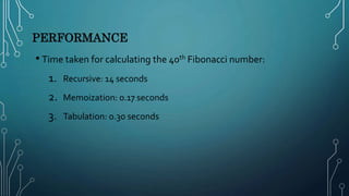
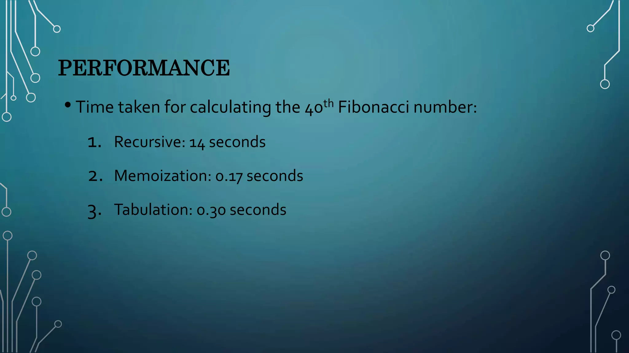
Time performance comparison for calculating Fibonacci numbers using recursive, memoization, and tabulation methods.
Concludes the presentation with a thank you note.


