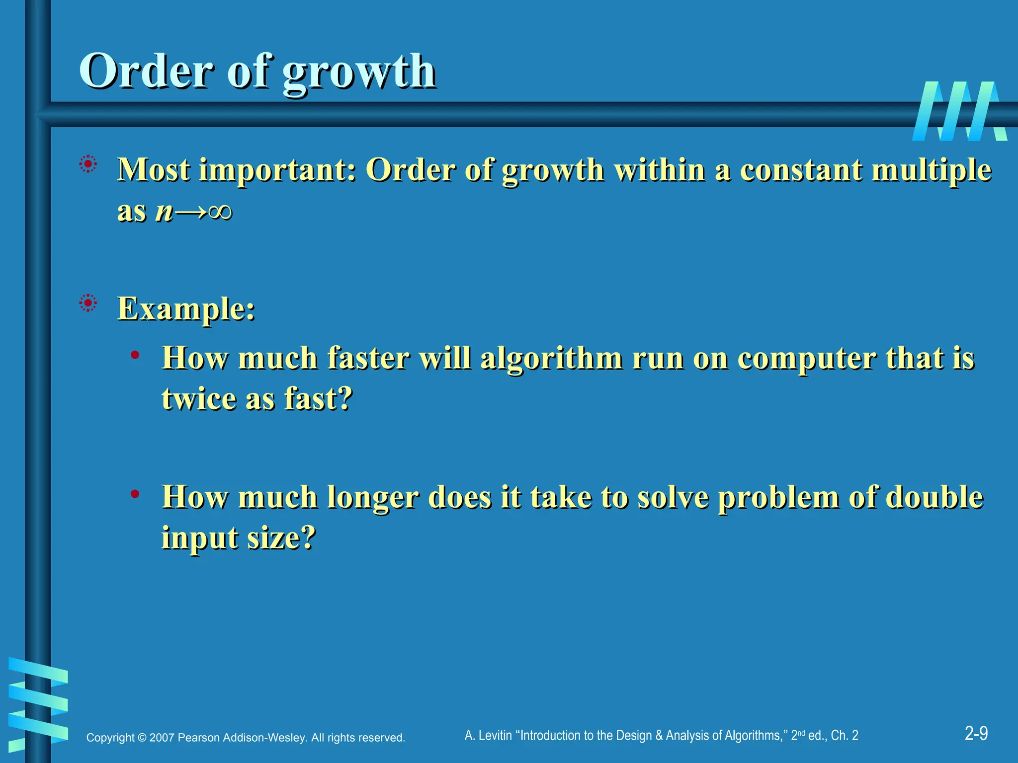
#9 Example: cn2
how much faster on twice as fast computer? (2)
how much longer for 2n? (4)
#15 Examples:
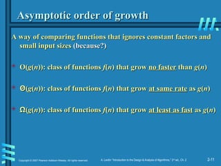
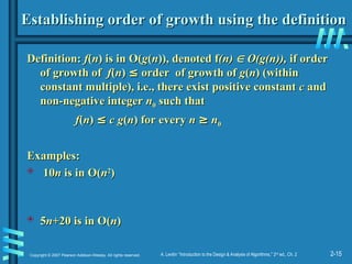
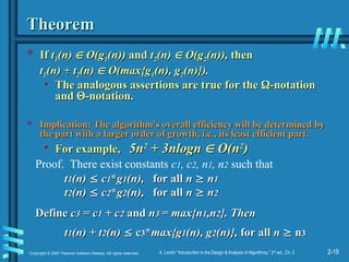
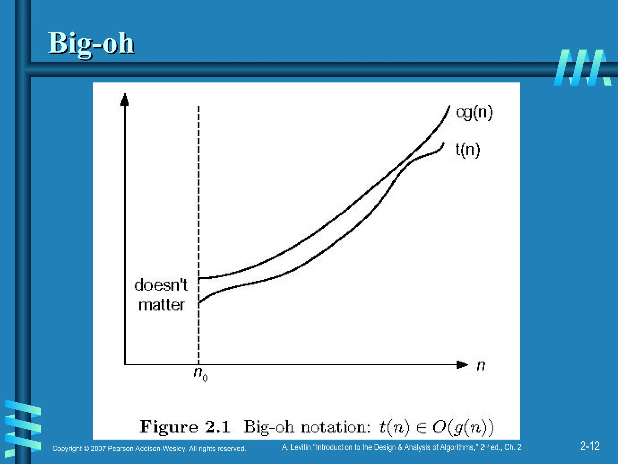
10n is O(n2)
since 10n ≤ 10n2 for n ≥ 1 or 10n ≤ n2 for n ≥ 10
c n0
5n+20 is O(10n)
since 5n+20 ≤ 10 n for n ≥ 4
c n0
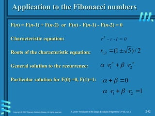
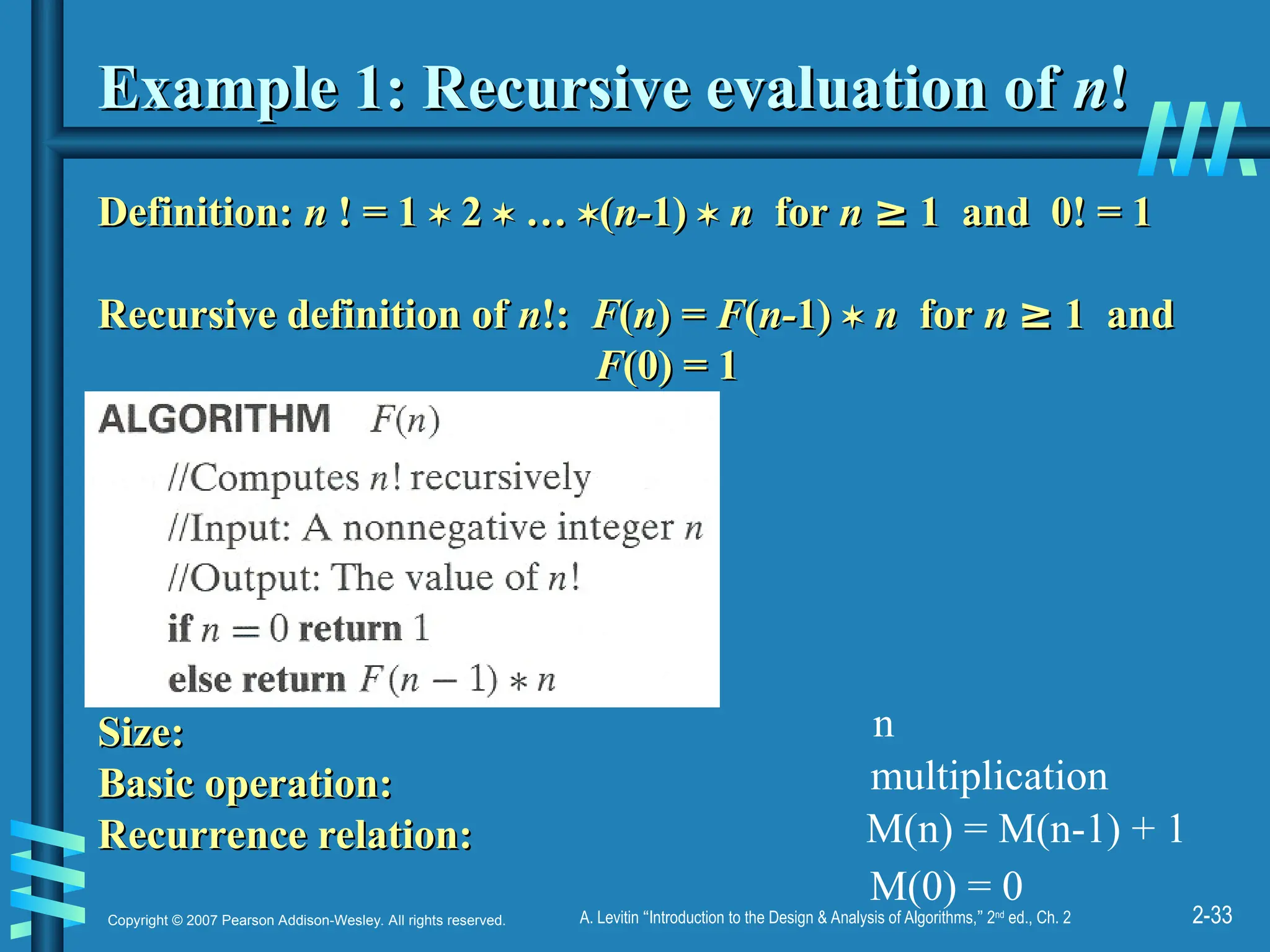
#33 Note the difference between the two recurrences. Students often confuse these!
F(n) = F(n-1) n
F(0) = 1
for the values of n!
------------
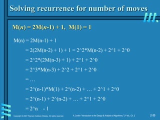
M(n) =M(n-1) + 1
M(0) = 0
for the number of multiplications made by this algorithm


![2-30
Copyright © 2007 Pearson Addison-Wesley. All rights reserved. A. Levitin “Introduction to the Design & Analysis of Algorithms,” 2nd
ed., Ch. 2
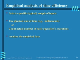
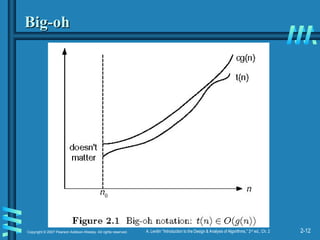
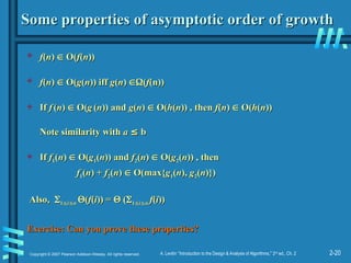
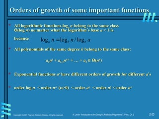
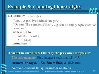
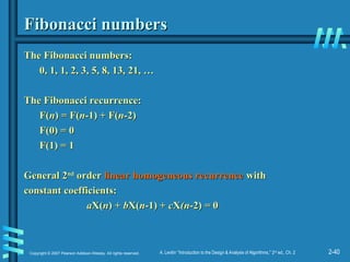
Example 4: Gaussian elimination
Example 4: Gaussian elimination
Algorithm
Algorithm GaussianElimination
GaussianElimination(
(A
A[0..
[0..n
n-
-1,0..
1,0..n
n])
])
//Implements Gaussian elimination on an
//Implements Gaussian elimination on an n-
n-by
by-
-(
(n
n+1) matrix
+1) matrix A
A
for
for i
i
0
0 to
to n
n -
- 2
2 do
do
for
for j
j
i
i + 1
+ 1 to
to n
n -
- 1
1 do
do
for
for k
k
i
i to
to n
n do
do
A
A[
[j
j,
,k
k]
]
A
A[
[j
j,
,k
k]
] -
- A
A[
[i
i,
,k
k]
]
A
A[
[j
j,
,i
i] /
] / A
A[
[i
i,
,i
i]
]
Find the efficiency class and a constant factor improvement.
Find the efficiency class and a constant factor improvement.
for
for i
i
0
0 to
to n
n -
- 2
2 do
do
for
for j
j
i
i + 1
+ 1 to
to n
n -
- 1
1 do
do
B
B
A
A[
[j,i
j,i] /
] / A
A[
[i
i,
,i
i]
]
for
for k
k
i
i to
to n
n do
do
A
A[
[j
j,
,k
k]
]
A
A[
[j
j,
,k
k]
] – A
– A[
[i,k
i,k]
] * B
* B](https://image.slidesharecdn.com/ch02n-250914130943-f83f672f/85/Fundamentals-of-the-analysis-of-algorithm-efficiency-30-320.jpg)


![2-45
Copyright © 2007 Pearson Addison-Wesley. All rights reserved. A. Levitin “Introduction to the Design & Analysis of Algorithms,” 2nd
ed., Ch. 2
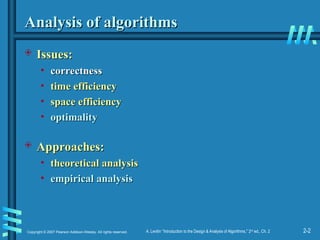
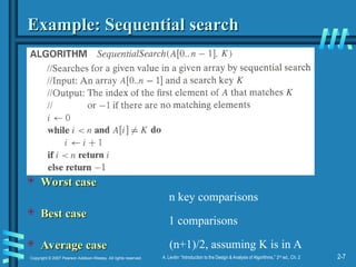
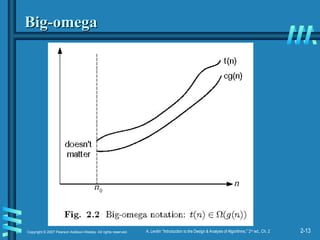
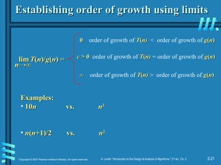
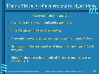
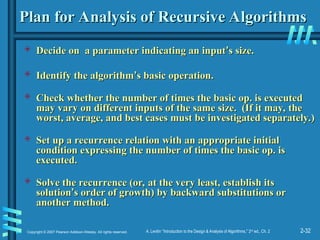
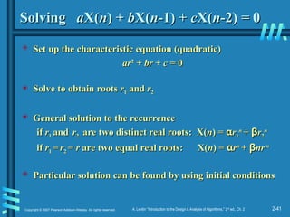
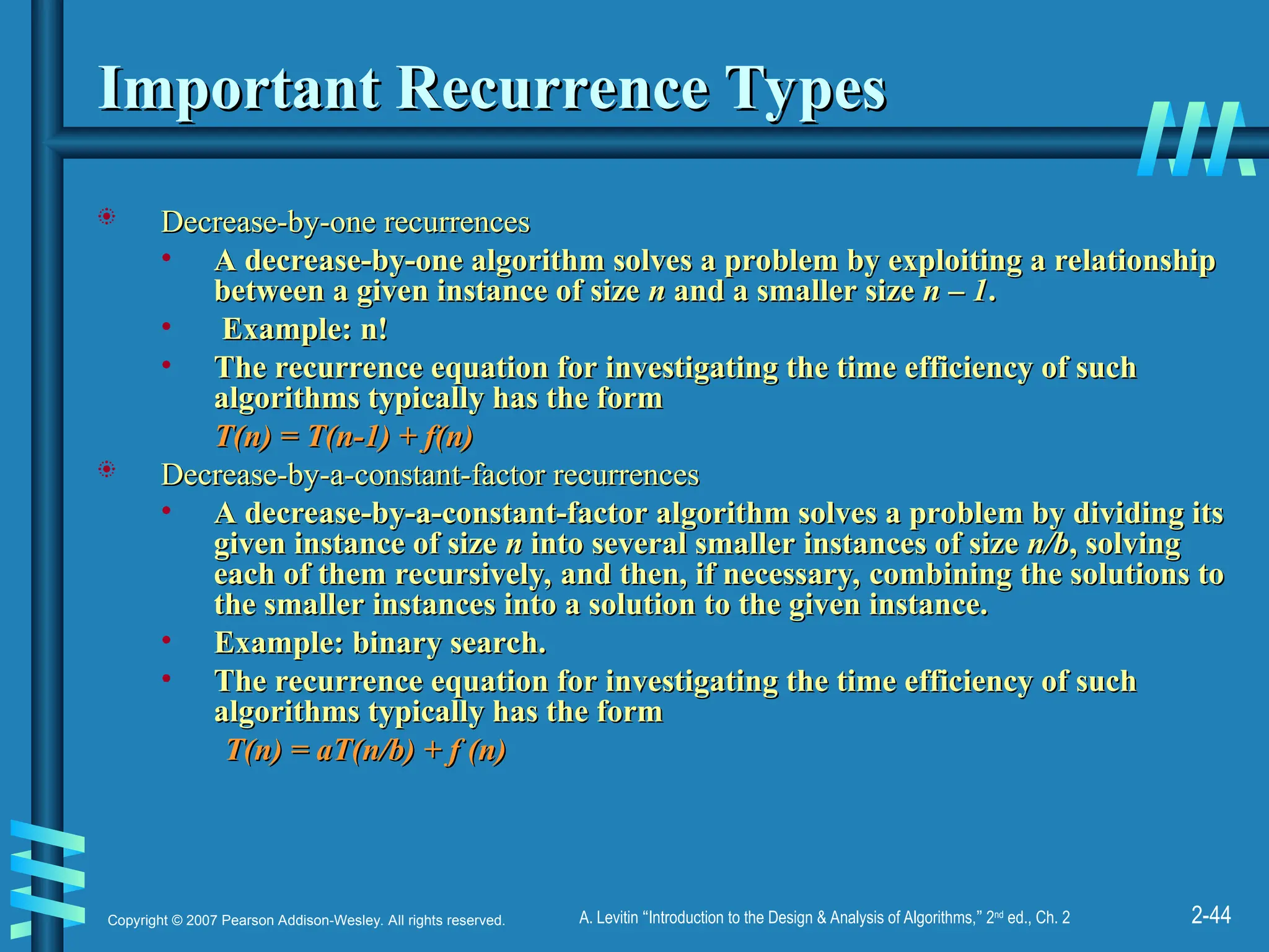
Decrease-by-one Recurrences
Decrease-by-one Recurrences
One (constant) operation reduces problem size by one.
One (constant) operation reduces problem size by one.
T(
T(n
n) = T(
) = T(n
n-1) +
-1) + c
c T(1) =
T(1) = d
d
Solution:
Solution:
A pass through input reduces problem size by one.
A pass through input reduces problem size by one.
T(
T(n
n) = T(
) = T(n
n-1) +
-1) + c n
c n T(1) =
T(1) = d
d
Solution:
Solution:
T(n) = (n-1)c + d linear
T(n) = [n(n+1)/2 – 1] c + d quadratic](https://image.slidesharecdn.com/ch02n-250914130943-f83f672f/85/Fundamentals-of-the-analysis-of-algorithm-efficiency-45-320.jpg)


![2-30
Copyright © 2007 Pearson Addison-Wesley. All rights reserved. A. Levitin “Introduction to the Design & Analysis of Algorithms,” 2nd
ed., Ch. 2
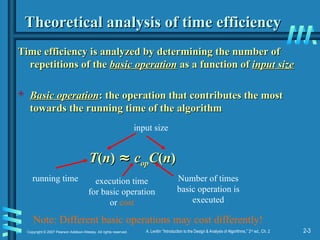
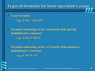
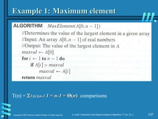
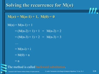
Example 4: Gaussian elimination
Example 4: Gaussian elimination
Algorithm
Algorithm GaussianElimination
GaussianElimination(
(A
A[0..
[0..n
n-
-1,0..
1,0..n
n])
])
//Implements Gaussian elimination on an
//Implements Gaussian elimination on an n-
n-by
by-
-(
(n
n+1) matrix
+1) matrix A
A
for
for i
i
0
0 to
to n
n -
- 2
2 do
do
for
for j
j
i
i + 1
+ 1 to
to n
n -
- 1
1 do
do
for
for k
k
i
i to
to n
n do
do
A
A[
[j
j,
,k
k]
]
A
A[
[j
j,
,k
k]
] -
- A
A[
[i
i,
,k
k]
]
A
A[
[j
j,
,i
i] /
] / A
A[
[i
i,
,i
i]
]
Find the efficiency class and a constant factor improvement.
Find the efficiency class and a constant factor improvement.
for
for i
i
0
0 to
to n
n -
- 2
2 do
do
for
for j
j
i
i + 1
+ 1 to
to n
n -
- 1
1 do
do
B
B
A
A[
[j,i
j,i] /
] / A
A[
[i
i,
,i
i]
]
for
for k
k
i
i to
to n
n do
do
A
A[
[j
j,
,k
k]
]
A
A[
[j
j,
,k
k]
] – A
– A[
[i,k
i,k]
] * B
* B](https://image.slidesharecdn.com/ch02n-250914130943-f83f672f/75/Fundamentals-of-the-analysis-of-algorithm-efficiency-30-2048.jpg)


![2-45
Copyright © 2007 Pearson Addison-Wesley. All rights reserved. A. Levitin “Introduction to the Design & Analysis of Algorithms,” 2nd
ed., Ch. 2
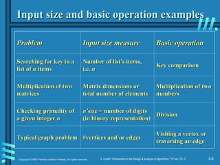
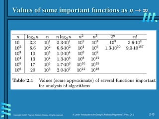
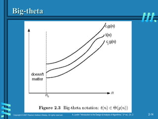
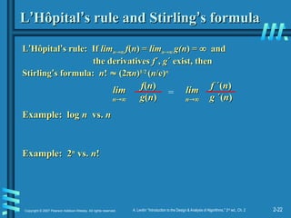
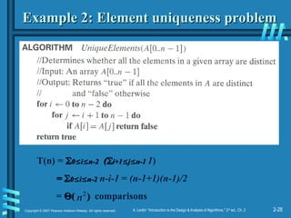
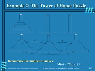
Decrease-by-one Recurrences
Decrease-by-one Recurrences
One (constant) operation reduces problem size by one.
One (constant) operation reduces problem size by one.
T(
T(n
n) = T(
) = T(n
n-1) +
-1) + c
c T(1) =
T(1) = d
d
Solution:
Solution:
A pass through input reduces problem size by one.
A pass through input reduces problem size by one.
T(
T(n
n) = T(
) = T(n
n-1) +
-1) + c n
c n T(1) =
T(1) = d
d
Solution:
Solution:
T(n) = (n-1)c + d linear
T(n) = [n(n+1)/2 – 1] c + d quadratic](https://image.slidesharecdn.com/ch02n-250914130943-f83f672f/75/Fundamentals-of-the-analysis-of-algorithm-efficiency-45-2048.jpg)