#4 Euclid’s algorithm is good for introducing the notion of an algorithm because it
makes a clear separation from a program that implements the algorithm.
It is also one that is familiar to most students.
Al Khowarizmi (many spellings possible...) – “algorism” (originally) and then
later “algorithm” come from his name.
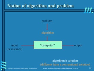
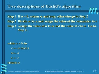
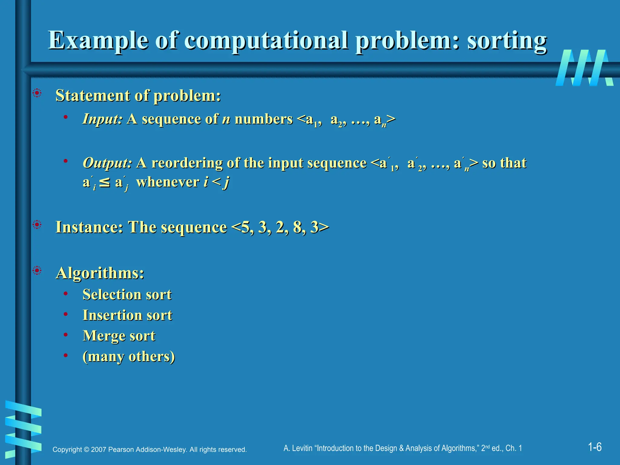
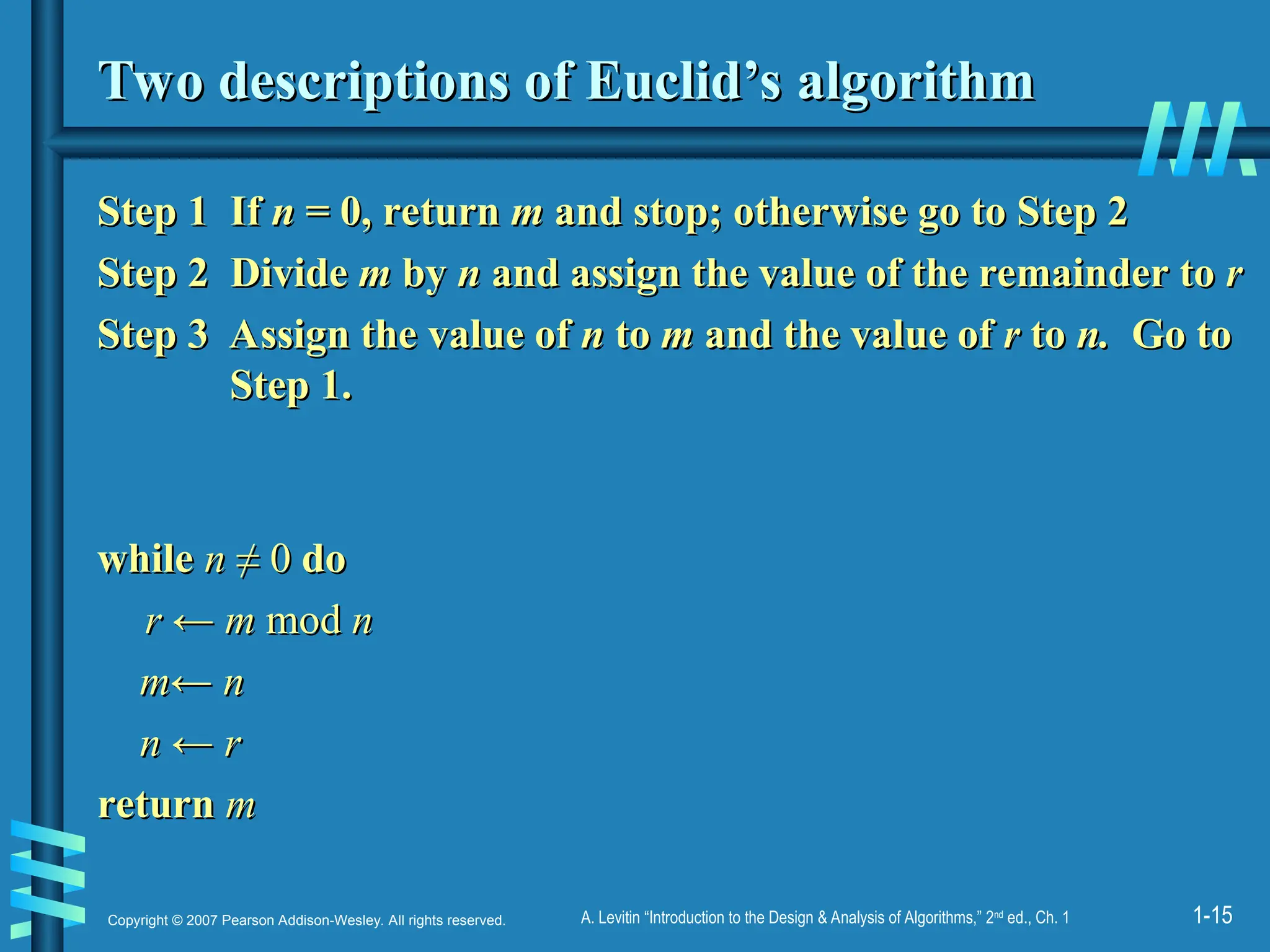
#7 The algorithm is given *very* informally here. Show students the pseudocode in
section 3.1.
This is a good opportunity to discuss pseudocode conventions.
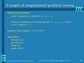
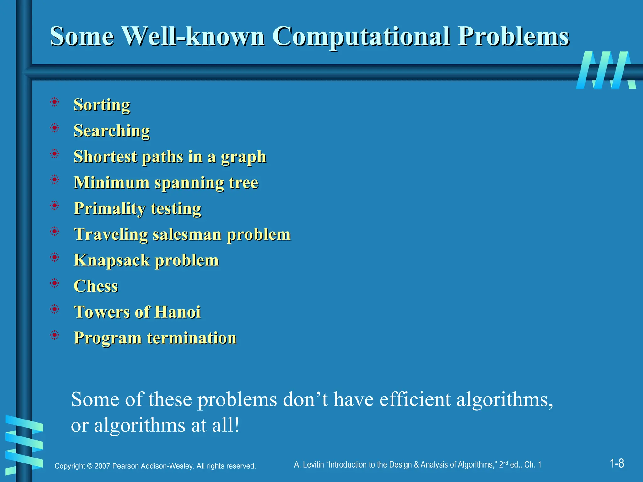
#8 1-4 have well known efficient (polynomial-time) solutions
5: primality testing has recently been found to have an efficient solution
This is a great problem to discuss because it has recently been in the news
(see mathworld news at: http://mathworld.wolfram.com/news/2002-08-07_primetest/
or original article: http://www.cse.iitk.ac.in/primality.pdf)
6(TSP)-9(chess) are all problems for which no efficient solution has been found
it is possible to informally discuss the “try all possibilities” approach that is required
to get exact solutions to such problems
10: Towers of Hanoi is a problem that has only exponential-time solutions (simply
because the output required is so large)
11: Program termination is undecidable
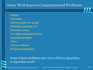
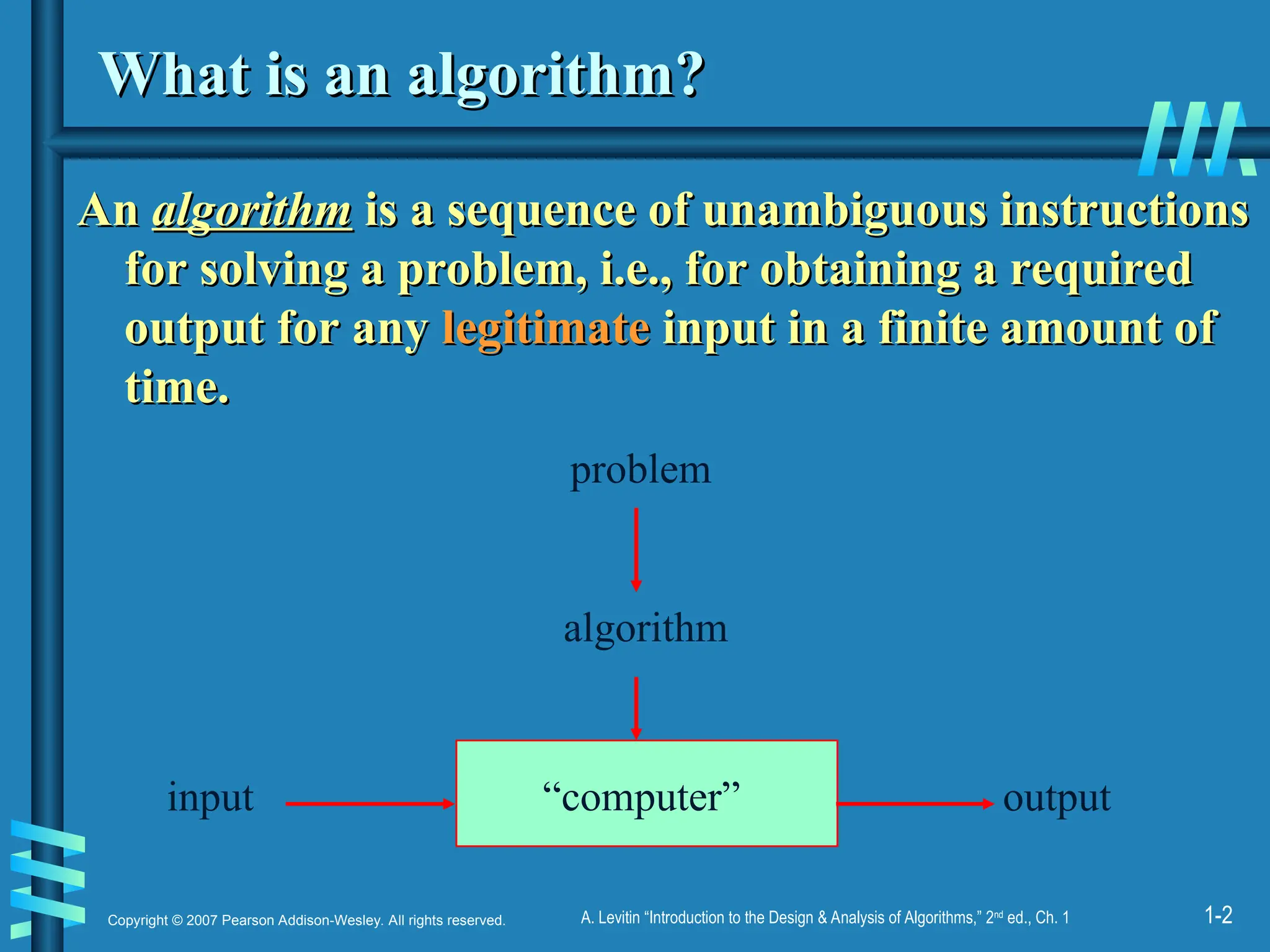
#12 The formalization of the notion of an algorithm led to great breakthroughs in the
foundations of mathematics in the 1930s.
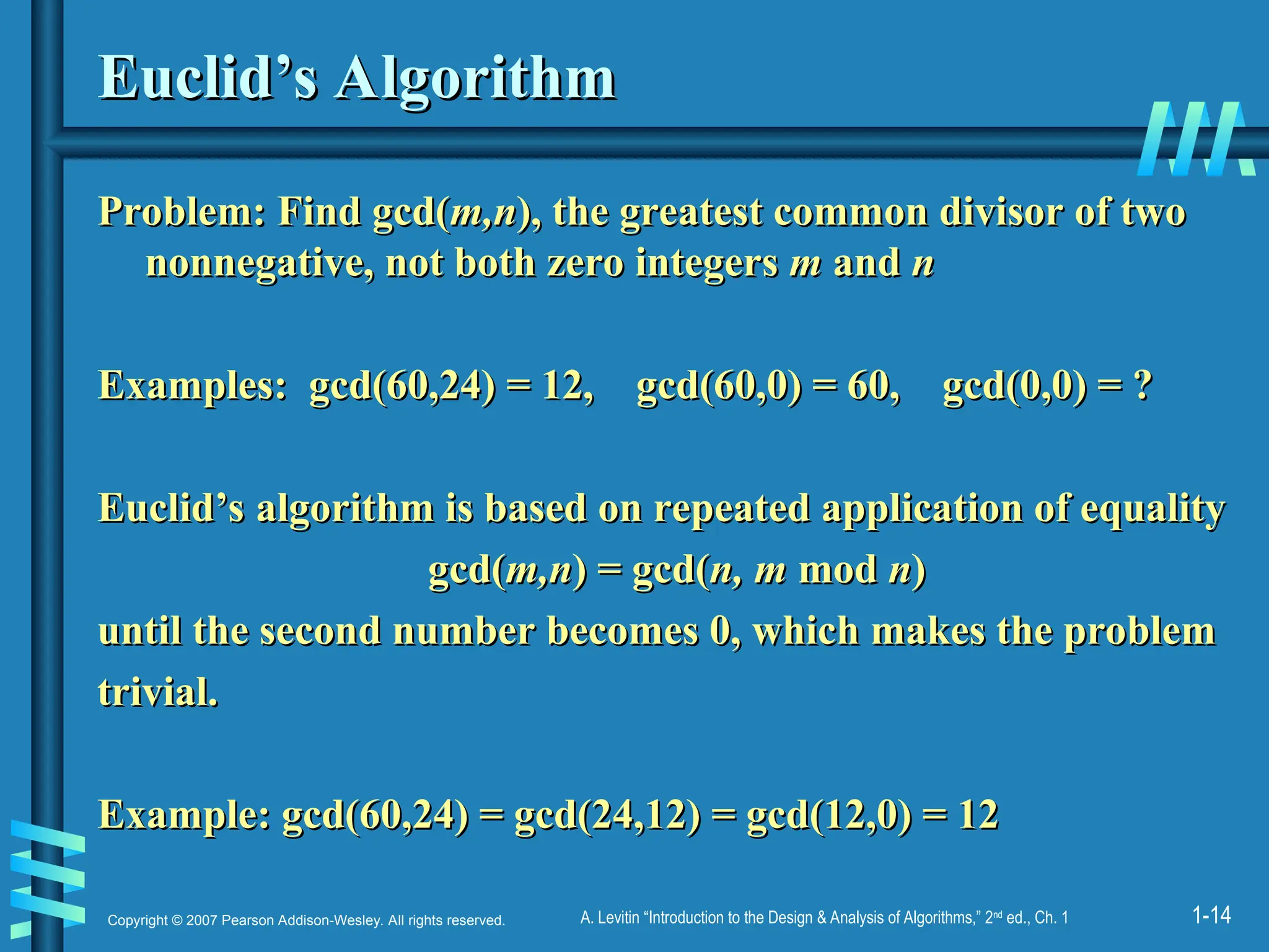
#14 Euclid’s algorithm is good for introducing the notion of an algorithm because it
makes a clear separation from a program that implements the algorithm.
It is also one that is familiar to most students.
Al Khowarizmi (many spellings possible...) – “algorism” (originally) and then
later “algorithm” come from his name.
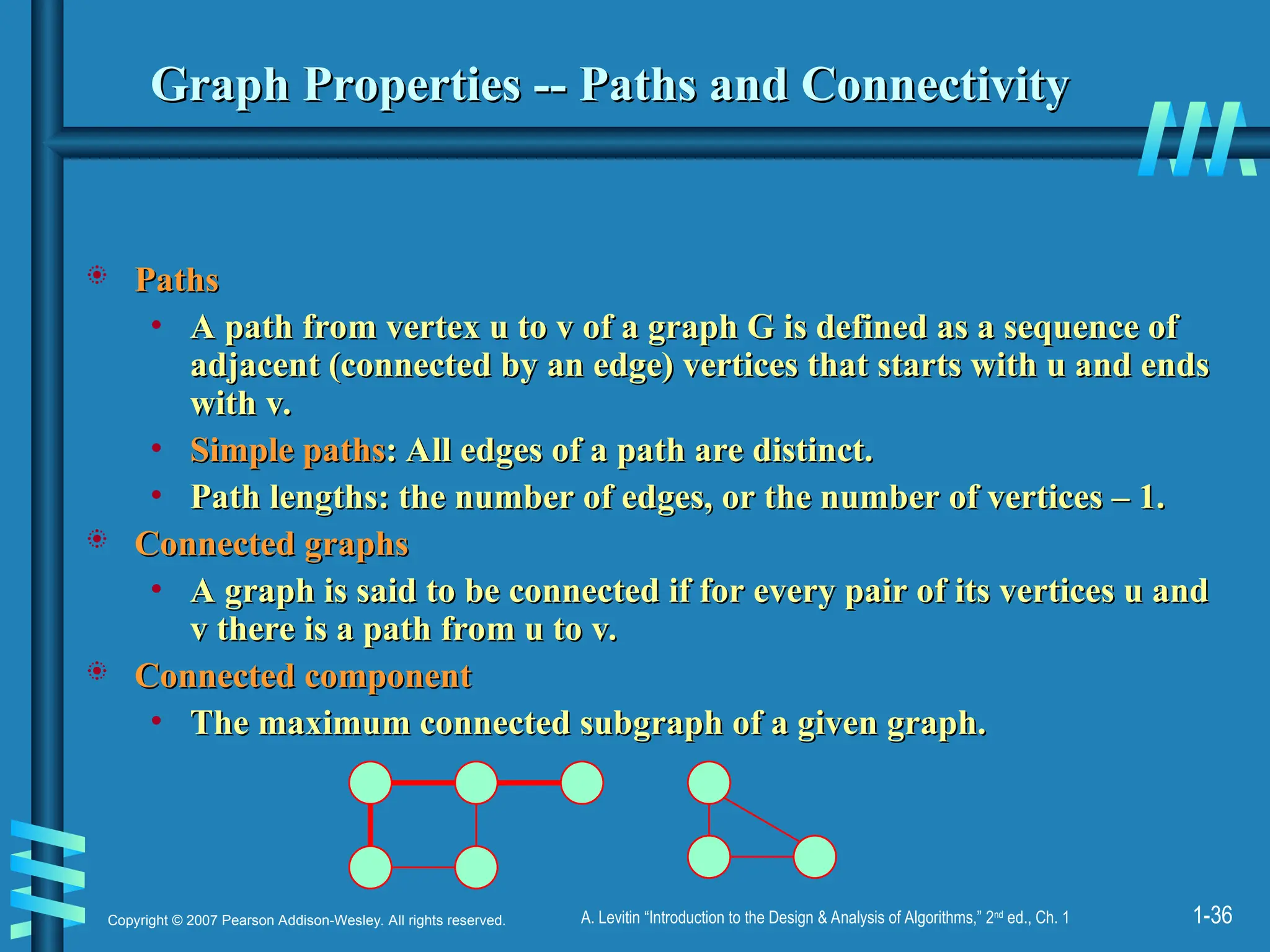
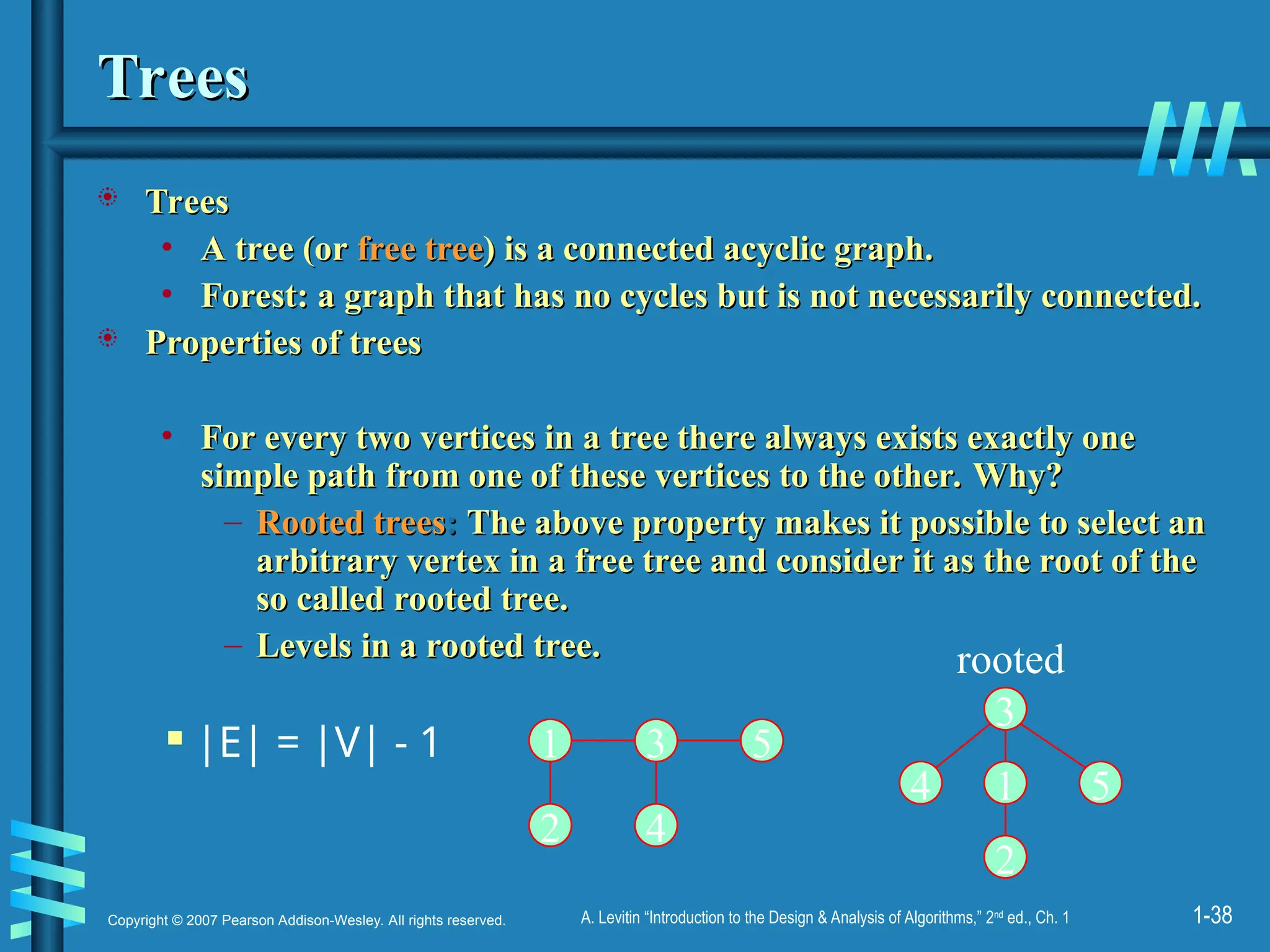
#36 Examples of a simple path and a not simple path.
Connected graphs: starting from any vertex, we can always find a path to reach all the other vertices. (Ball-String example.)
From NIST:
Connected graphs:
Definition: An undirected graph that has a path between every pair of vertices.
Strongly connected graphs:
Definition: A directed graph that has a path from each vertex to every other vertex.
Connected component: …
Strongly connected component:
a strongly connected component of a digraph G is a maximal strongly connected subgraph of G.


![1-7
Copyright © 2007 Pearson Addison-Wesley. All rights reserved. A. Levitin “Introduction to the Design & Analysis of Algorithms,” 2nd
ed., Ch. 1
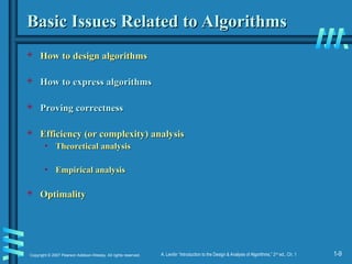
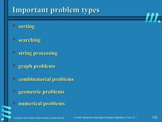
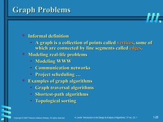
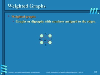
Selection Sort
Selection Sort
Input: array
Input: array a[1],…,a[n]
a[1],…,a[n]
Output: array
Output: array a
a sorted in non-decreasing order
sorted in non-decreasing order
Algorithm:
Algorithm:
for i=1 to n
swap a[i] with smallest of a[i],…,a[n]
• Is this unambiguous? Effective?
• See also pseudocode, section 3.1](https://image.slidesharecdn.com/ch01n-250914130728-73ea05a5/85/introduction-design-and-analysis-algorithm-7-320.jpg)


![1-17
Copyright © 2007 Pearson Addison-Wesley. All rights reserved. A. Levitin “Introduction to the Design & Analysis of Algorithms,” 2nd
ed., Ch. 1
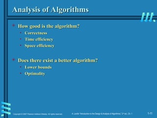
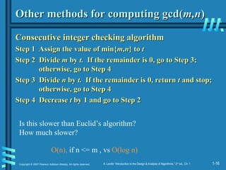
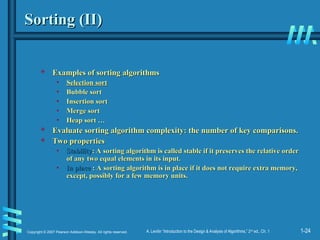
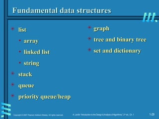
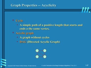
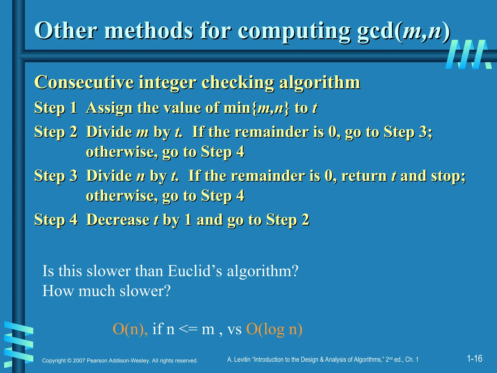
Other methods for gcd(
Other methods for gcd(m,n
m,n) [cont.]
) [cont.]
Middle-school procedure
Middle-school procedure
Step 1 Find the prime factorization of
Step 1 Find the prime factorization of m
m
Step 2 Find the prime factorization of
Step 2 Find the prime factorization of n
n
Step 3 Find all the common prime factors
Step 3 Find all the common prime factors
Step 4 Compute the product of all the common prime factors
Step 4 Compute the product of all the common prime factors
and return it as gcd
and return it as gcd(m,n
(m,n)
)
Is this an algorithm?
Is this an algorithm?
How efficient is it?
How efficient is it?
Time complexity: O(sqrt(n))](https://image.slidesharecdn.com/ch01n-250914130728-73ea05a5/85/introduction-design-and-analysis-algorithm-17-320.jpg)
![1-18
Copyright © 2007 Pearson Addison-Wesley. All rights reserved. A. Levitin “Introduction to the Design & Analysis of Algorithms,” 2nd
ed., Ch. 1
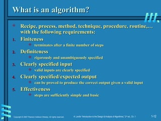
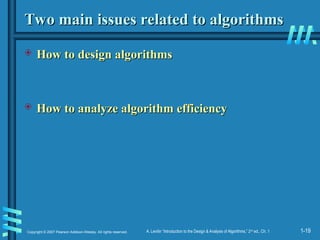
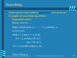
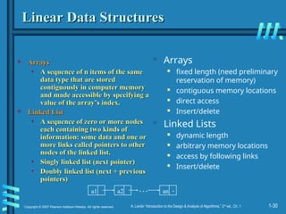
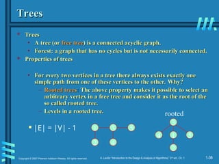
Sieve of Eratosthenes
Sieve of Eratosthenes
Input:
Input: Integer
Integer n
n ≥
≥ 2
2
Output: List of primes less than or equal to
Output: List of primes less than or equal to n
n
for
for p
p ← 2
← 2 to
to n
n do
do A
A[
[p
p] ←
] ← p
p
for
for p
p ← 2
← 2 to
to n
n do
do
if
if A
A[
[p
p]
]
0 //
0 //p
p hasn’t been previously eliminated from the list
hasn’t been previously eliminated from the list
j
j ←
← p
p*
* p
p
while
while j
j ≤
≤ n
n do
do
A
A[
[j
j]
] ← 0
← 0 //mark element as eliminated
//mark element as eliminated
j
j ←
← j
j + p
+ p
Example: 2 3 4 5 6 7 8 9 10 11 12 13 14 15 16 17 18 19 20
Example: 2 3 4 5 6 7 8 9 10 11 12 13 14 15 16 17 18 19 20
Time complexity: O(n)](https://image.slidesharecdn.com/ch01n-250914130728-73ea05a5/85/introduction-design-and-analysis-algorithm-18-320.jpg)


![1-25
Copyright © 2007 Pearson Addison-Wesley. All rights reserved. A. Levitin “Introduction to the Design & Analysis of Algorithms,” 2nd
ed., Ch. 1
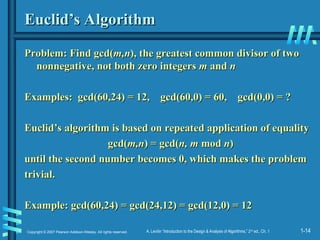
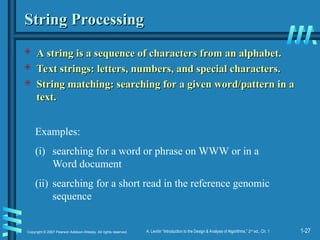
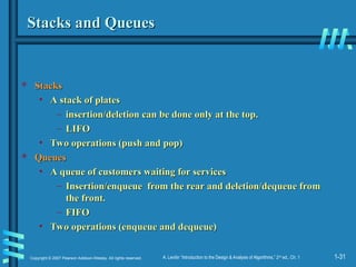
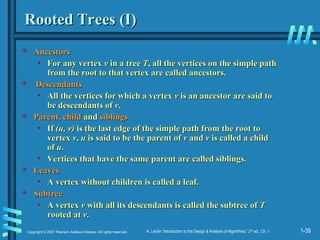
Selection Sort
Selection Sort
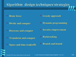
Algorithm
Algorithm SelectionSort(A[0..n-1])
SelectionSort(A[0..n-1])
//The algorithm sorts a given array by selection sort
//The algorithm sorts a given array by selection sort
//Input: An array A[0..n-1] of orderable elements
//Input: An array A[0..n-1] of orderable elements
//Output: Array A[0..n-1] sorted in ascending order
//Output: Array A[0..n-1] sorted in ascending order
for i
for i
0 to n – 2 do
0 to n – 2 do
min
min
i
i
for j
for j
i + 1 to n – 1 do
i + 1 to n – 1 do
if A[j] < A[min]
if A[j] < A[min]
min
min
j
j
swap A[i] and A[min]
swap A[i] and A[min]](https://image.slidesharecdn.com/ch01n-250914130728-73ea05a5/85/introduction-design-and-analysis-algorithm-25-320.jpg)


![1-7
Copyright © 2007 Pearson Addison-Wesley. All rights reserved. A. Levitin “Introduction to the Design & Analysis of Algorithms,” 2nd
ed., Ch. 1
Selection Sort
Selection Sort
Input: array
Input: array a[1],…,a[n]
a[1],…,a[n]
Output: array
Output: array a
a sorted in non-decreasing order
sorted in non-decreasing order
Algorithm:
Algorithm:
for i=1 to n
swap a[i] with smallest of a[i],…,a[n]
• Is this unambiguous? Effective?
• See also pseudocode, section 3.1](https://image.slidesharecdn.com/ch01n-250914130728-73ea05a5/75/introduction-design-and-analysis-algorithm-7-2048.jpg)

![1-17
Copyright © 2007 Pearson Addison-Wesley. All rights reserved. A. Levitin “Introduction to the Design & Analysis of Algorithms,” 2nd
ed., Ch. 1
Other methods for gcd(
Other methods for gcd(m,n
m,n) [cont.]
) [cont.]
Middle-school procedure
Middle-school procedure
Step 1 Find the prime factorization of
Step 1 Find the prime factorization of m
m
Step 2 Find the prime factorization of
Step 2 Find the prime factorization of n
n
Step 3 Find all the common prime factors
Step 3 Find all the common prime factors
Step 4 Compute the product of all the common prime factors
Step 4 Compute the product of all the common prime factors
and return it as gcd
and return it as gcd(m,n
(m,n)
)
Is this an algorithm?
Is this an algorithm?
How efficient is it?
How efficient is it?
Time complexity: O(sqrt(n))](https://image.slidesharecdn.com/ch01n-250914130728-73ea05a5/75/introduction-design-and-analysis-algorithm-17-2048.jpg)
![1-18
Copyright © 2007 Pearson Addison-Wesley. All rights reserved. A. Levitin “Introduction to the Design & Analysis of Algorithms,” 2nd
ed., Ch. 1
Sieve of Eratosthenes
Sieve of Eratosthenes
Input:
Input: Integer
Integer n
n ≥
≥ 2
2
Output: List of primes less than or equal to
Output: List of primes less than or equal to n
n
for
for p
p ← 2
← 2 to
to n
n do
do A
A[
[p
p] ←
] ← p
p
for
for p
p ← 2
← 2 to
to n
n do
do
if
if A
A[
[p
p]
]
0 //
0 //p
p hasn’t been previously eliminated from the list
hasn’t been previously eliminated from the list
j
j ←
← p
p*
* p
p
while
while j
j ≤
≤ n
n do
do
A
A[
[j
j]
] ← 0
← 0 //mark element as eliminated
//mark element as eliminated
j
j ←
← j
j + p
+ p
Example: 2 3 4 5 6 7 8 9 10 11 12 13 14 15 16 17 18 19 20
Example: 2 3 4 5 6 7 8 9 10 11 12 13 14 15 16 17 18 19 20
Time complexity: O(n)](https://image.slidesharecdn.com/ch01n-250914130728-73ea05a5/75/introduction-design-and-analysis-algorithm-18-2048.jpg)

![1-25
Copyright © 2007 Pearson Addison-Wesley. All rights reserved. A. Levitin “Introduction to the Design & Analysis of Algorithms,” 2nd
ed., Ch. 1
Selection Sort
Selection Sort
Algorithm
Algorithm SelectionSort(A[0..n-1])
SelectionSort(A[0..n-1])
//The algorithm sorts a given array by selection sort
//The algorithm sorts a given array by selection sort
//Input: An array A[0..n-1] of orderable elements
//Input: An array A[0..n-1] of orderable elements
//Output: Array A[0..n-1] sorted in ascending order
//Output: Array A[0..n-1] sorted in ascending order
for i
for i
0 to n – 2 do
0 to n – 2 do
min
min
i
i
for j
for j
i + 1 to n – 1 do
i + 1 to n – 1 do
if A[j] < A[min]
if A[j] < A[min]
min
min
j
j
swap A[i] and A[min]
swap A[i] and A[min]](https://image.slidesharecdn.com/ch01n-250914130728-73ea05a5/75/introduction-design-and-analysis-algorithm-25-2048.jpg)