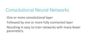
Downloaded 366 times

![Overfitting Mitigation
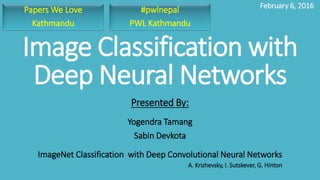
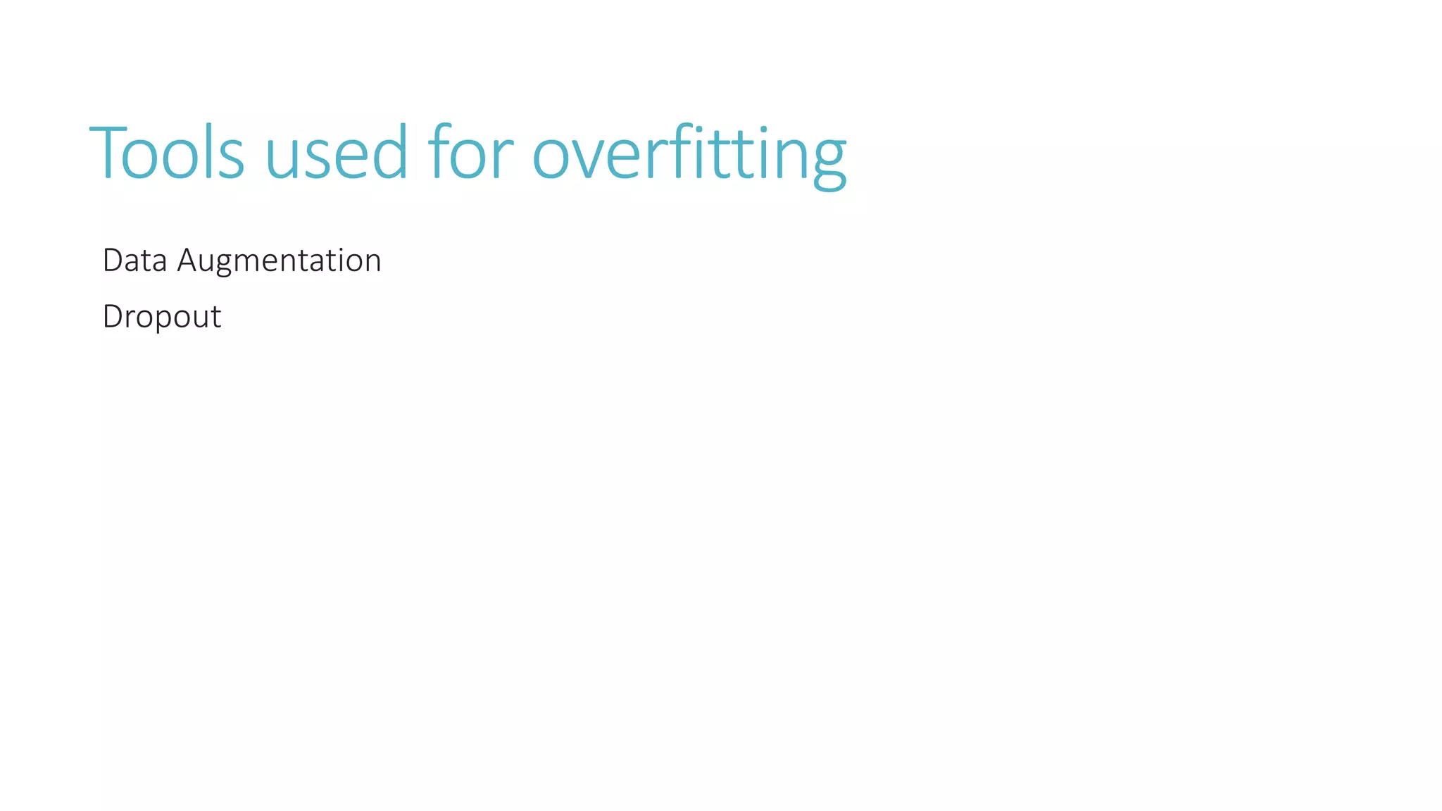
Data Augmentation :
Artificially creating more data samples from existing data through various
transformation of images (i.e. rotation, reflection, skewing etc.) and/or dividing
images into small patches and averaging all their predictions.
Applying PCA to the training examples to find out principal components which
correspond to intensity and color of the illumination. Creating artificial data by
adding randomly scaled eigen vectors to the training examples.
𝐼𝑥𝑦 𝑅, 𝐼𝑥𝑦 𝐺, 𝐼𝑥𝑦 𝐵 𝑇 = 𝒑𝟏, 𝒑𝟐, 𝒑𝟑 [𝛼1 𝜆1, 𝛼2 𝜆2, 𝛼3 𝜆3] 𝑇
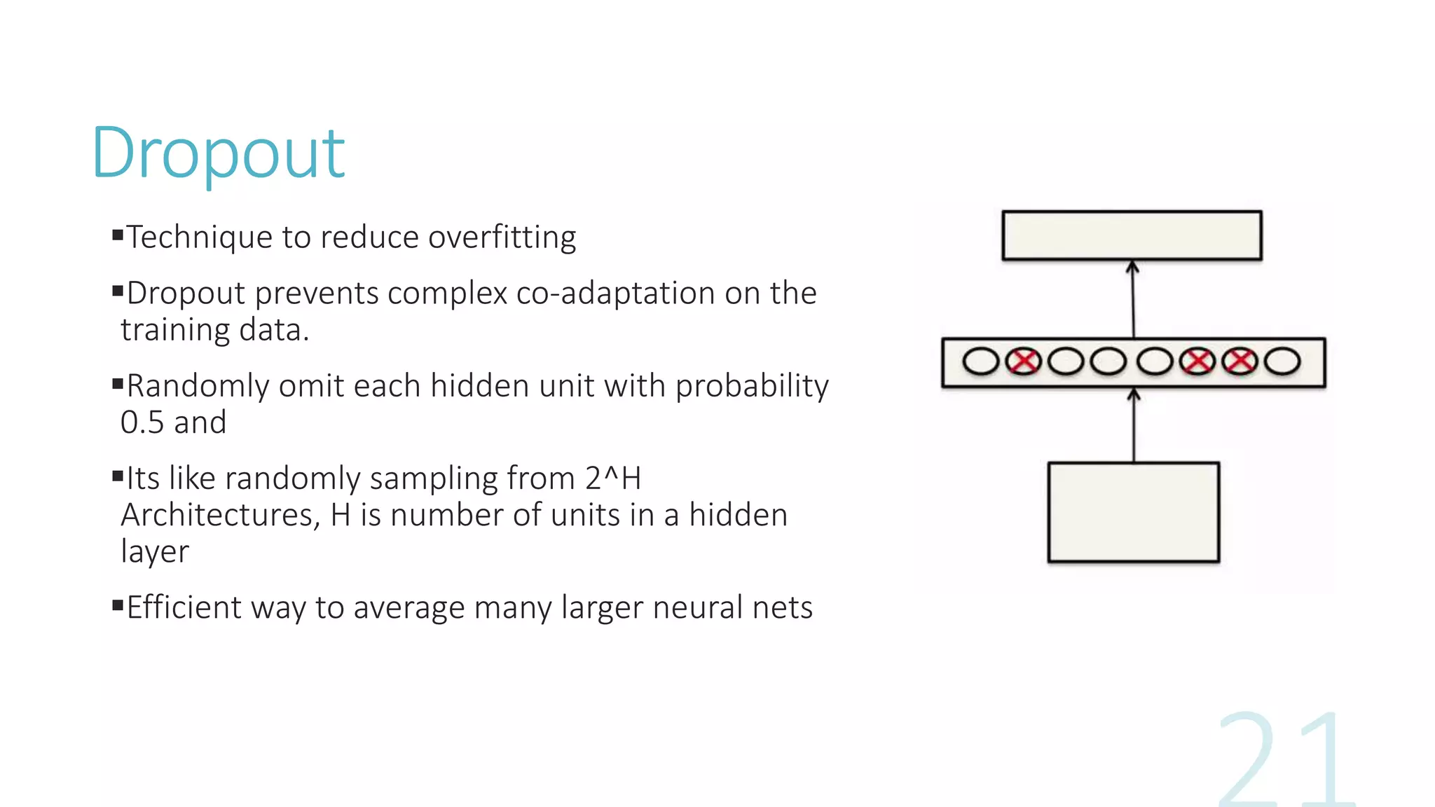
Dropout:](https://image.slidesharecdn.com/imageclassification-160206090009/85/Image-classification-with-Deep-Neural-Networks-18-320.jpg)

![References[1] A. Krizhevsky, I. Sutskever and G. E. Hinton, "ImageNet Classification with Deep Convolutional Neural
Networks," 2012.
[2] S. Tara, Brian Kingsbury, A.-r. Mohamed and B. Ramabhadran, "Learning Filter Banks within a Deep Neural
Network Framework," in IEEE, 2013.
[3] A. Graves, A.-r. Mohamed and G. Hinton, "Speech Recognition with Deep Recurrent Neural Networks,"
University of Toronto.
[4] A. Graves, "Generating Sequences with Recurrent Neural Networks," arXiv, 2014.
[5] Q. V. Oriol Vinyals, "A Neural Conversational Model," arXiv, 2015.
[6] R. Grishick, J. Donahue, T. Darrel and J. Mallik, "Rich Features Hierarchies for accurate object detection and
semantic segmentation.," UC Berkeley.
[7] A. Karpathy, "CS231n Convolutional Neural Networks for Visual Recognition," Stanford University, [Online].
Available: http://cs231n.github.io/convolutional-networks/.
[8] I. Sutskever, "Training Recurrent Neural Networks," University of Toronto, 2013.
[9] "Convolutional Neural Networks (LeNet)," [Online]. Available: http://deeplearning.net/tutorial/lenet.html.
[10] C. Eugenio, A. Dundar, J. Jin and J. Bates, "An Analysis of the Connections Between Layers of Deep Neural
Networks," arXiv, 2013.](https://image.slidesharecdn.com/imageclassification-160206090009/85/Image-classification-with-Deep-Neural-Networks-28-320.jpg)
![References
[11] M. D. Zeiler and F. Rob, "Visualizing and Understanding Convolutional Networks," arXiv, 2013.
[12] G. Hinton, N. Srivastava, A. Karpathy, I. Sutskever and R. Salakhutdinov, Improving Neural Networks
by preventing co-adaptation of feature detectors, Totonto: arXiv, 2012.
[13] L. Fie-Fie. and A. Karpathy, "Deep Visual Alignment for Generating Image Descriptions,"
Standford University, 2014.
[14] O. Vinyals, A. Toshev., S. Bengio and D. Erthan, "Show and Tell: A Neural Image Caption
Generator.," Google Inc., 2014.
[15] J. M. G. H. IIya Sutskever, "Generating Text with Recurrent Neural Networks," in 28th International
Conference on Machine Learning, Bellevue, 2011.
[16] "Theano," [Online]. Available: http://deeplearning.net/software/theano/index.html. [Accessed 27
10 2015].
[17] "What is GPU Computing ?," NVIDIA, [Online]. Available: http://www.nvidia.com/object/what-is-
gpu-computing.html. [Accessed 27 12 2015].
[18] "GeForce 820M|Specifications," NVIDIA, [Online]. Available:
http://www.geforce.com/hardware/notebook-gpus/geforce-820m/specifications. [Accessed 28
10 2015].](https://image.slidesharecdn.com/imageclassification-160206090009/85/Image-classification-with-Deep-Neural-Networks-29-320.jpg)


![Overfitting Mitigation
Data Augmentation :
Artificially creating more data samples from existing data through various
transformation of images (i.e. rotation, reflection, skewing etc.) and/or dividing
images into small patches and averaging all their predictions.
Applying PCA to the training examples to find out principal components which
correspond to intensity and color of the illumination. Creating artificial data by
adding randomly scaled eigen vectors to the training examples.
𝐼𝑥𝑦 𝑅, 𝐼𝑥𝑦 𝐺, 𝐼𝑥𝑦 𝐵 𝑇 = 𝒑𝟏, 𝒑𝟐, 𝒑𝟑 [𝛼1 𝜆1, 𝛼2 𝜆2, 𝛼3 𝜆3] 𝑇
Dropout:](https://image.slidesharecdn.com/imageclassification-160206090009/75/Image-classification-with-Deep-Neural-Networks-18-2048.jpg)
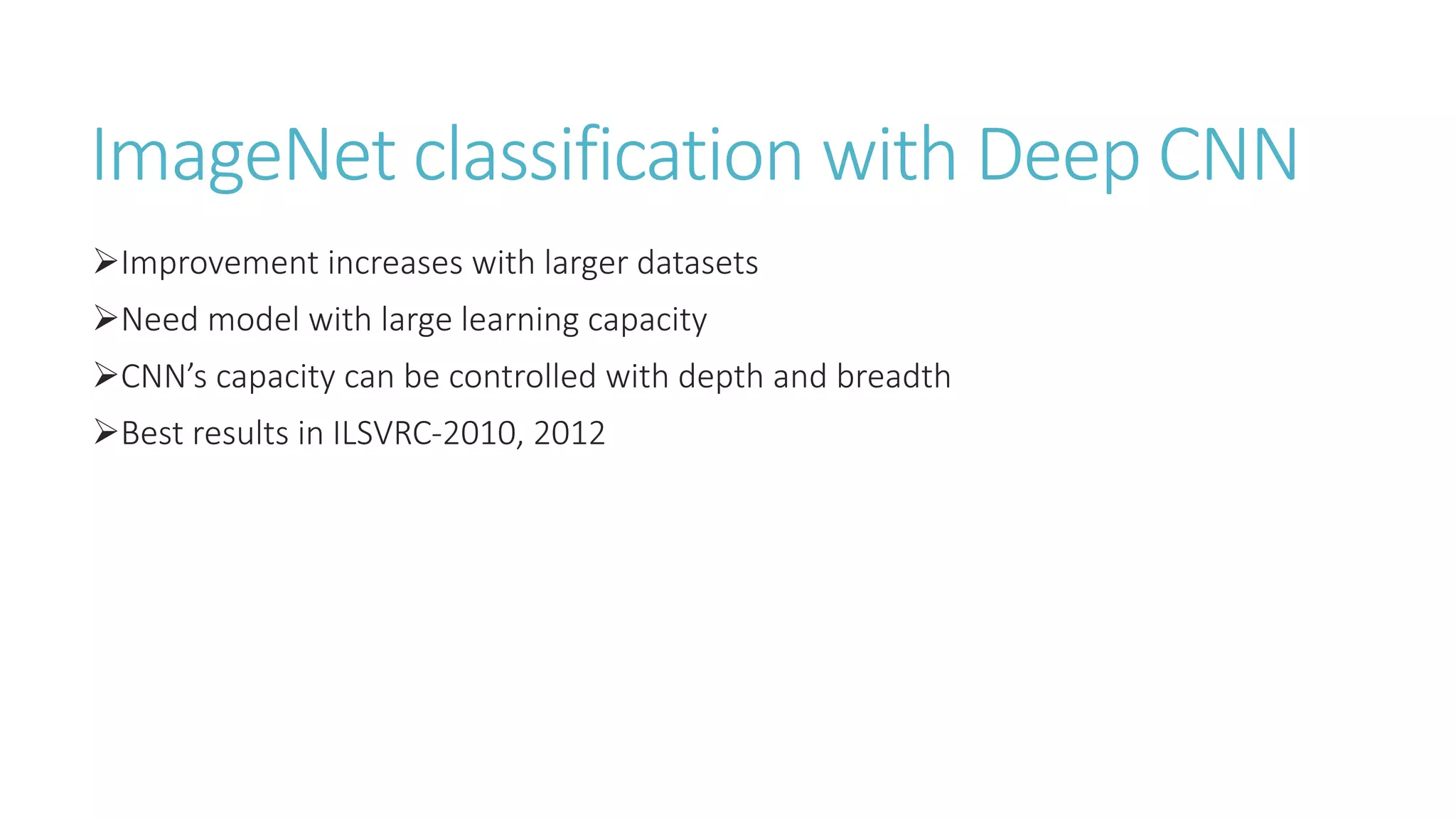

![References[1] A. Krizhevsky, I. Sutskever and G. E. Hinton, "ImageNet Classification with Deep Convolutional Neural
Networks," 2012.
[2] S. Tara, Brian Kingsbury, A.-r. Mohamed and B. Ramabhadran, "Learning Filter Banks within a Deep Neural
Network Framework," in IEEE, 2013.
[3] A. Graves, A.-r. Mohamed and G. Hinton, "Speech Recognition with Deep Recurrent Neural Networks,"
University of Toronto.
[4] A. Graves, "Generating Sequences with Recurrent Neural Networks," arXiv, 2014.
[5] Q. V. Oriol Vinyals, "A Neural Conversational Model," arXiv, 2015.
[6] R. Grishick, J. Donahue, T. Darrel and J. Mallik, "Rich Features Hierarchies for accurate object detection and
semantic segmentation.," UC Berkeley.
[7] A. Karpathy, "CS231n Convolutional Neural Networks for Visual Recognition," Stanford University, [Online].
Available: http://cs231n.github.io/convolutional-networks/.
[8] I. Sutskever, "Training Recurrent Neural Networks," University of Toronto, 2013.
[9] "Convolutional Neural Networks (LeNet)," [Online]. Available: http://deeplearning.net/tutorial/lenet.html.
[10] C. Eugenio, A. Dundar, J. Jin and J. Bates, "An Analysis of the Connections Between Layers of Deep Neural
Networks," arXiv, 2013.](https://image.slidesharecdn.com/imageclassification-160206090009/75/Image-classification-with-Deep-Neural-Networks-28-2048.jpg)
![References
[11] M. D. Zeiler and F. Rob, "Visualizing and Understanding Convolutional Networks," arXiv, 2013.
[12] G. Hinton, N. Srivastava, A. Karpathy, I. Sutskever and R. Salakhutdinov, Improving Neural Networks
by preventing co-adaptation of feature detectors, Totonto: arXiv, 2012.
[13] L. Fie-Fie. and A. Karpathy, "Deep Visual Alignment for Generating Image Descriptions,"
Standford University, 2014.
[14] O. Vinyals, A. Toshev., S. Bengio and D. Erthan, "Show and Tell: A Neural Image Caption
Generator.," Google Inc., 2014.
[15] J. M. G. H. IIya Sutskever, "Generating Text with Recurrent Neural Networks," in 28th International
Conference on Machine Learning, Bellevue, 2011.
[16] "Theano," [Online]. Available: http://deeplearning.net/software/theano/index.html. [Accessed 27
10 2015].
[17] "What is GPU Computing ?," NVIDIA, [Online]. Available: http://www.nvidia.com/object/what-is-
gpu-computing.html. [Accessed 27 12 2015].
[18] "GeForce 820M|Specifications," NVIDIA, [Online]. Available:
http://www.geforce.com/hardware/notebook-gpus/geforce-820m/specifications. [Accessed 28
10 2015].](https://image.slidesharecdn.com/imageclassification-160206090009/75/Image-classification-with-Deep-Neural-Networks-29-2048.jpg)

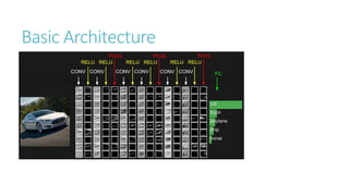
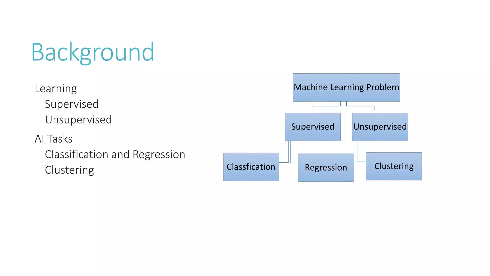
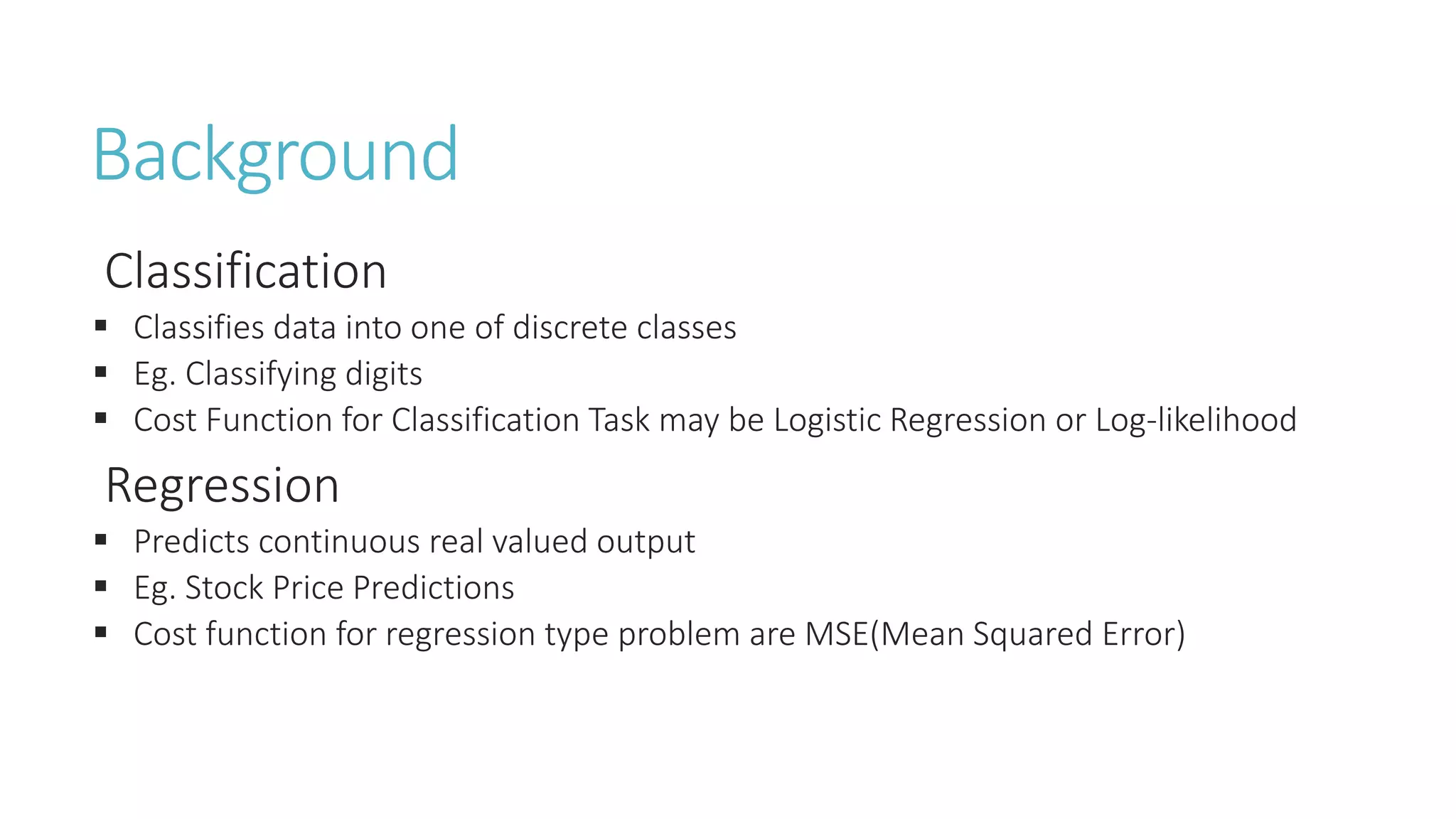
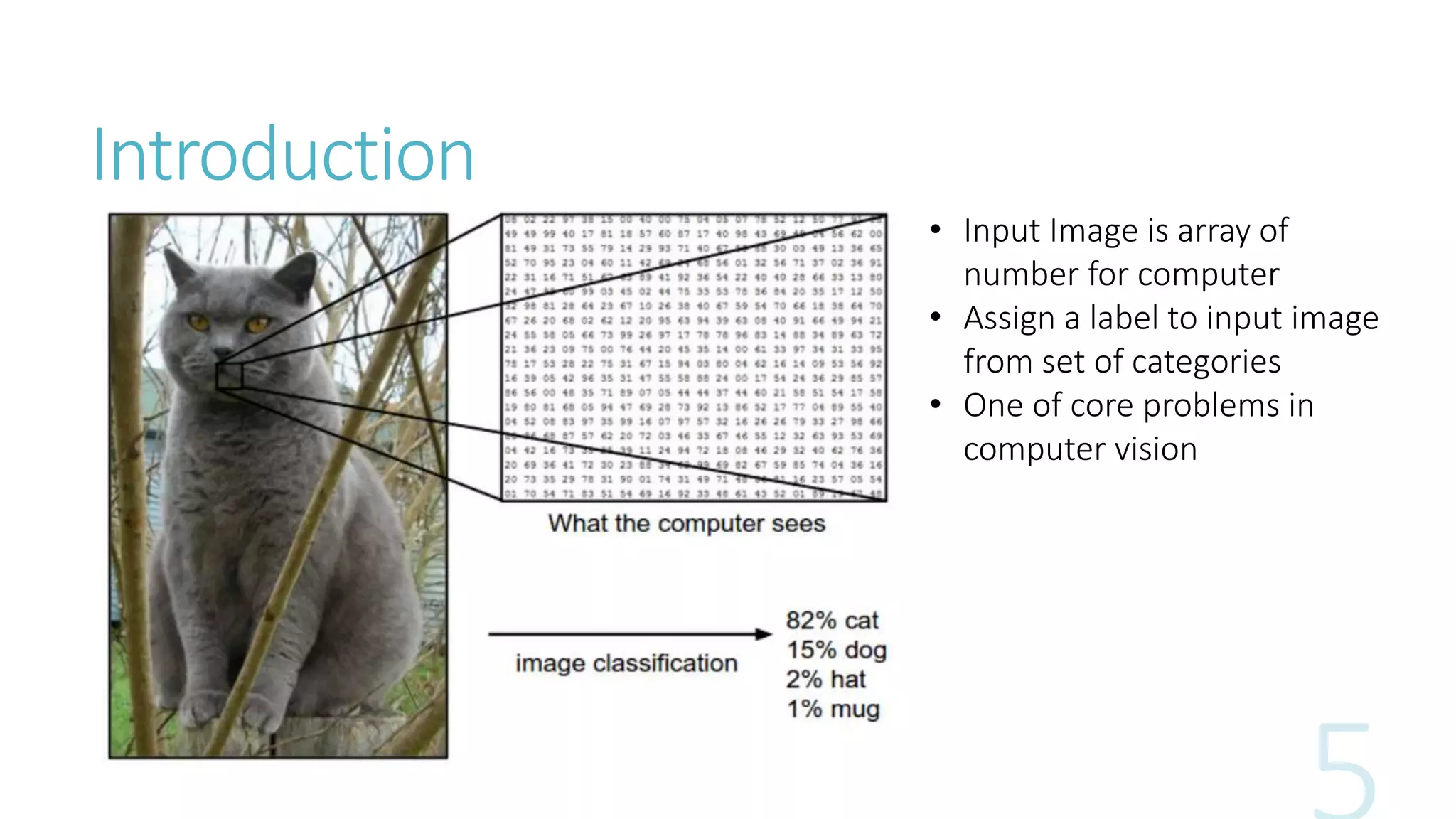
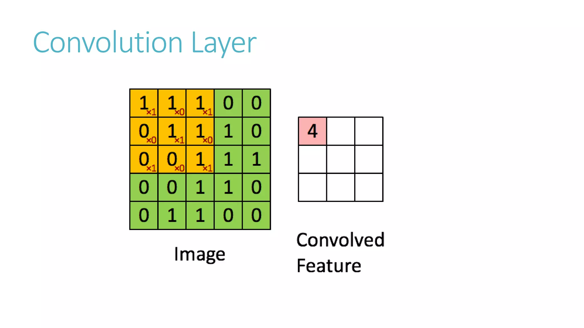
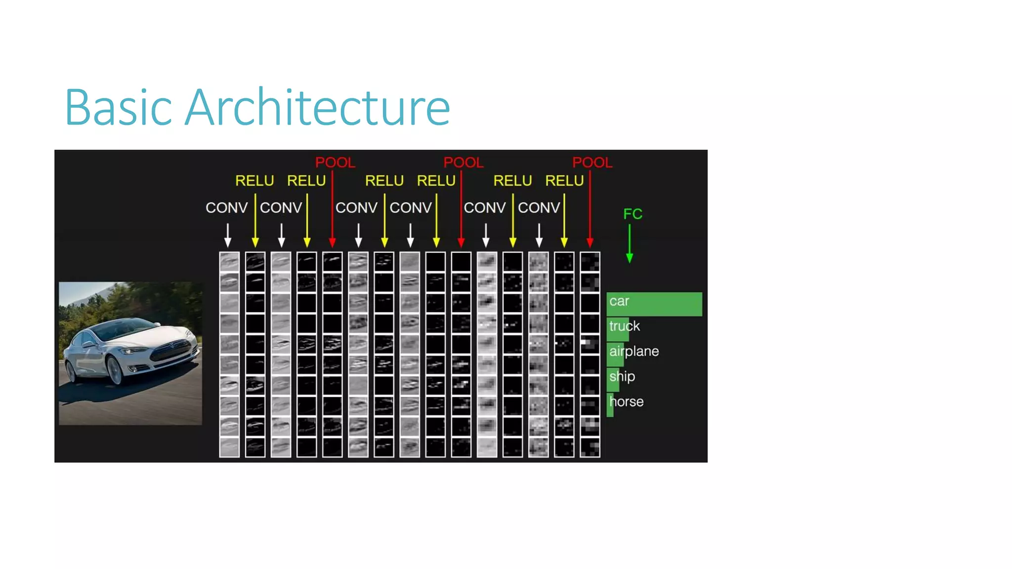
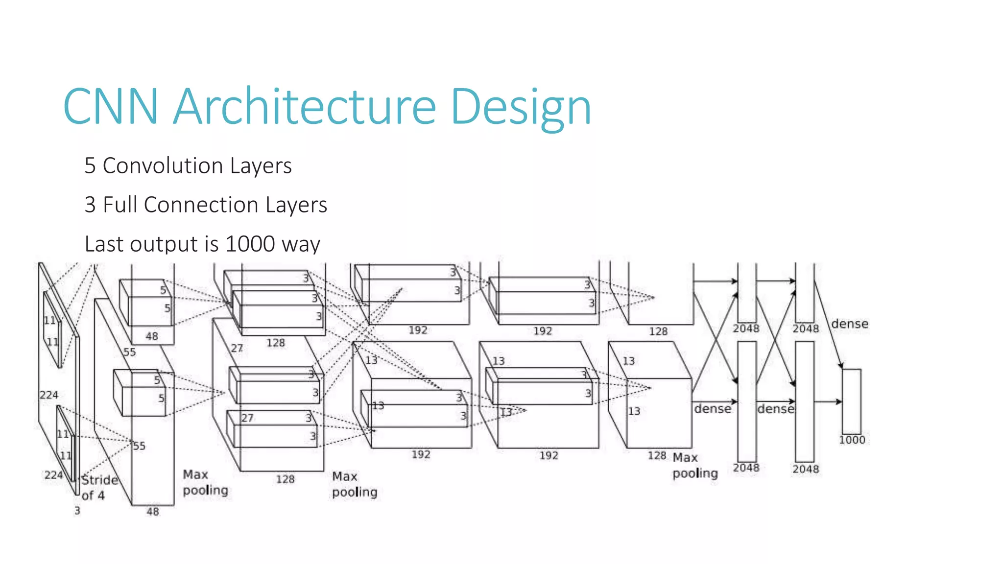
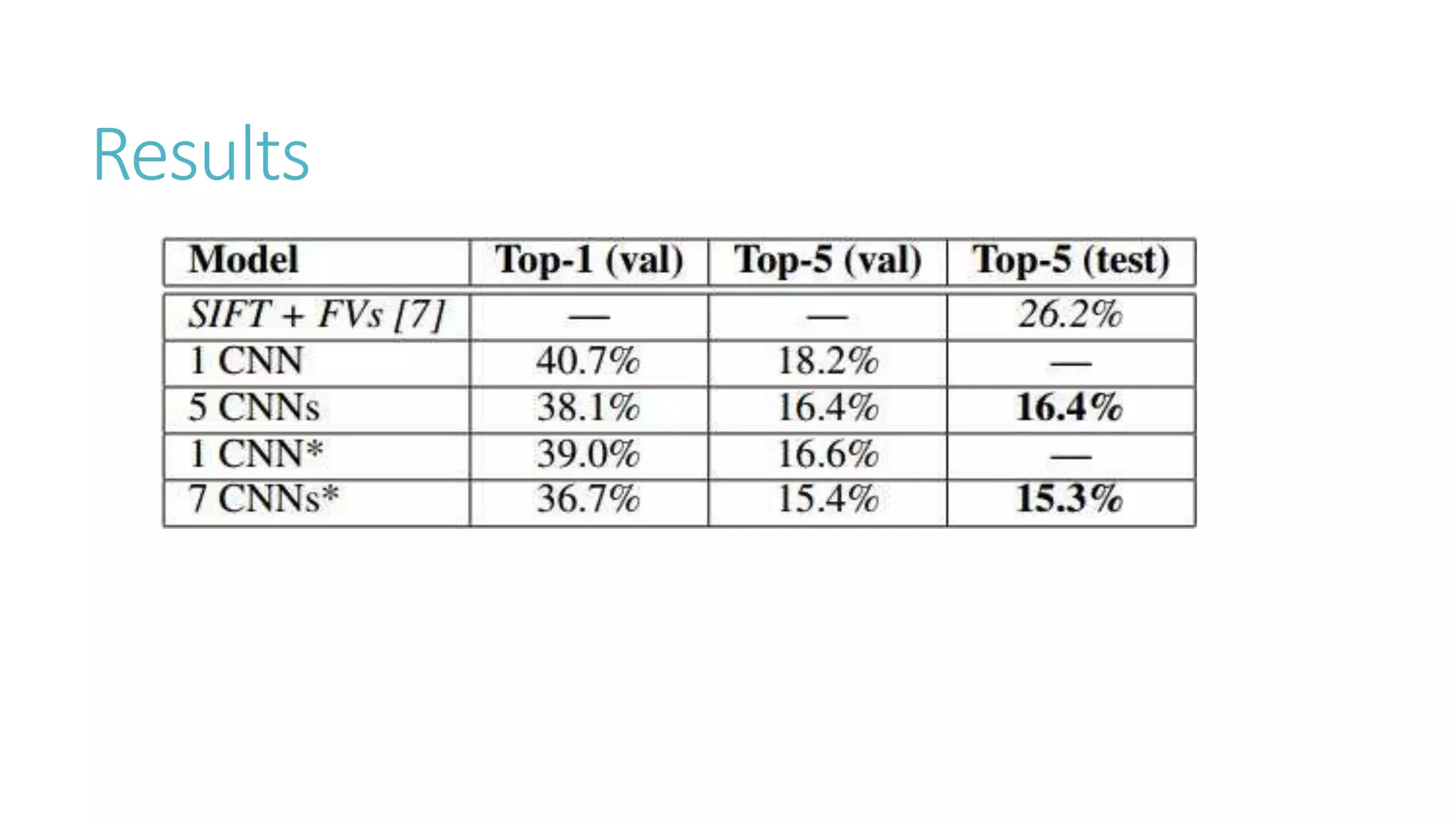
This document discusses image classification using deep neural networks. It provides background on image classification and convolutional neural networks. The document outlines techniques like activation functions, pooling, dropout and data augmentation to prevent overfitting. It summarizes a paper on ImageNet classification using CNNs with multiple convolutional and fully connected layers. The paper achieved state-of-the-art results on ImageNet in 2010 and 2012 by training CNNs on a large dataset using multiple GPUs.


