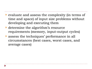
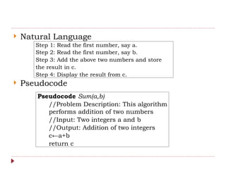
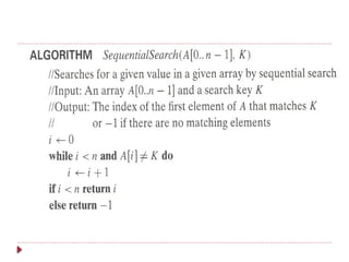
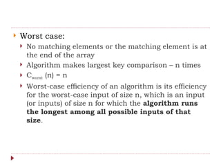
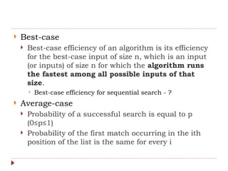
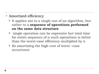
The document provides an overview of algorithm design and analysis, defining concepts such as algorithms, their qualities, and characteristics. It discusses the importance of non-ambiguity, efficiency, and various algorithmic strategies, as well as the need for careful problem evaluation and different algorithm types. Additionally, it addresses algorithm efficiency in both time and space, discussing methods of analysis and problem types commonly encountered in computing.
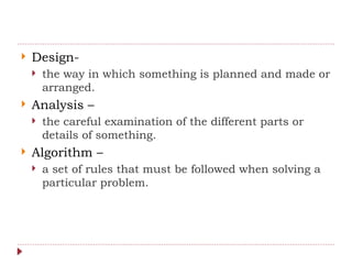
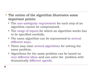
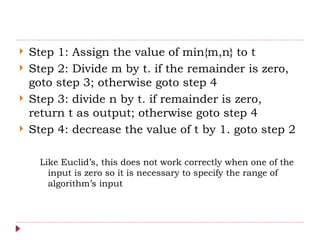
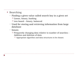
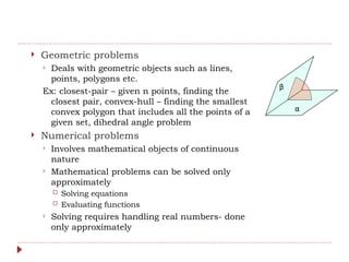
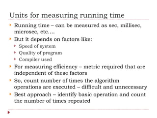
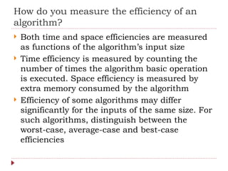
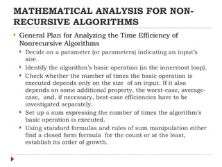
![# include<stdio.h>
int find_odd(int k)
{ int n=0,n1,n2;
while (n!=-1) {
scanf("%d",&n);
if(n%2==1) {
n1++;
if(n1==k) {
return n;
break; } }
else if(n==-1) {
return n;
break; }
else
continue; }}
void main()
{
int a[100],i,k;
scanf("%d",&k);
printf("%d",find_odd(k));
}](https://image.slidesharecdn.com/daa-241210041622-7f759d36/85/Introduction-to-Design-and-Analysis-of-Algorithms-9-320.jpg)


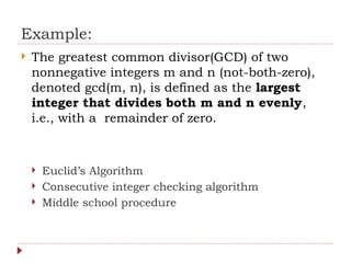


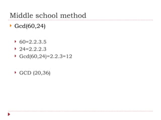


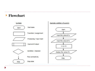


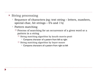
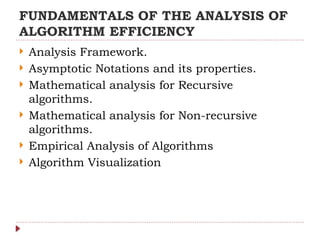
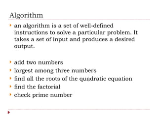
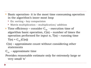
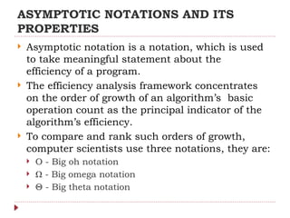
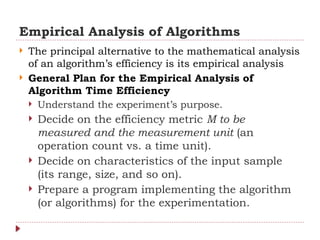
![ Spell checking algorithm, if examines individual
char –
number of char
Processing words – number of words
Algorithm involving numbers – checking a number
n is prime or not – use number of bits in the binary
representation
b=[log2n]+1](https://image.slidesharecdn.com/daa-241210041622-7f759d36/85/Introduction-to-Design-and-Analysis-of-Algorithms-43-320.jpg)
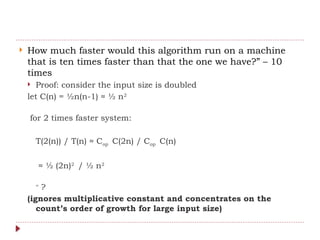
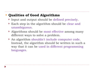
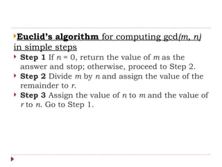
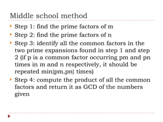
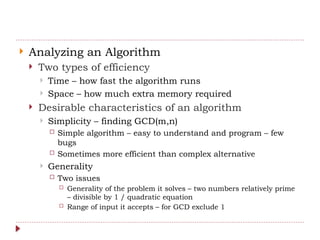
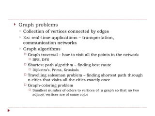
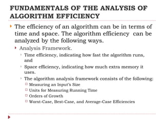
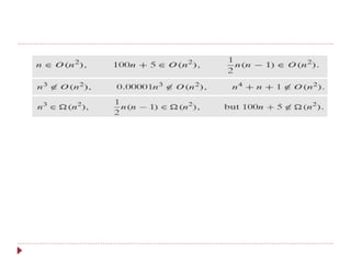
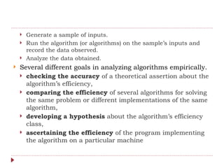
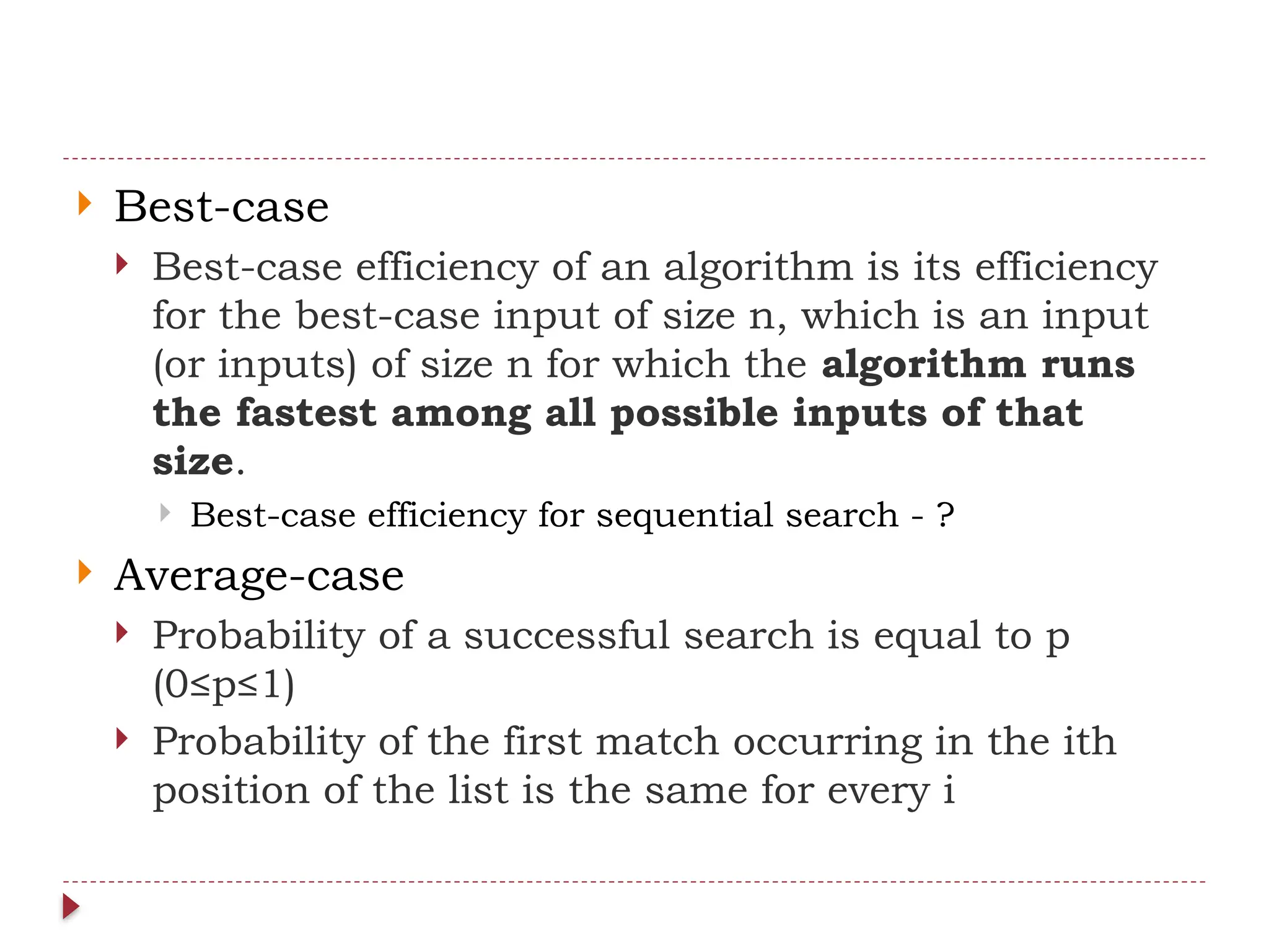
![ Calculating Cavg (n):
Successful search = p/n for every i
Unsuccessful search = (1-p)
Cavg (n) = [1.p/n+…n.p/n]+n.(1-p)
= p/n [1+…+n]+n(1-p)
= p/n n(n+1)/2 +n(1-p)
= p(n+1)/2+n(1-p)
When p=1 =?
When p=0 =?
Average case is not the average of best and worst case
efficiencies](https://image.slidesharecdn.com/daa-241210041622-7f759d36/85/Introduction-to-Design-and-Analysis-of-Algorithms-55-320.jpg)
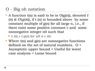
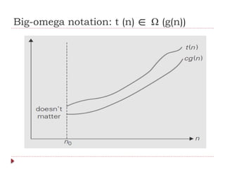
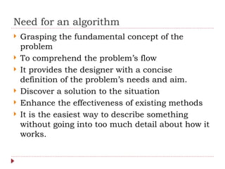
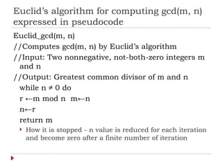
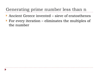
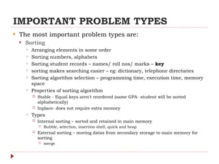
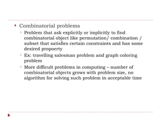
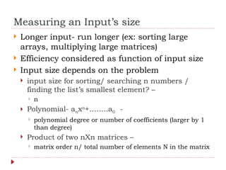
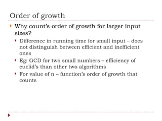
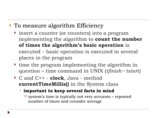
![Useful Property Involving the Asymptotic
Notations
THEOREM: If t1(n) O(g1(n)) and t2(n) O(g2(n)), then t1(n) + t2(n)
∈ ∈ ∈
O(max{g1(n), g2(n)}). (The analogous assertions are true for the Ω and Θ notations
as well.)
PROOF: The proof extends to orders of growth the following simple fact about four
arbitrary real numbers a1, b1, a2, b2: if a1 ≤ b1 and a2 ≤ b2, then a1 + a2 ≤ 2
max{b1, b2}.
Since t1(n) O(g1(n)), there exist some positive constant c1 and some nonnegative integer
∈
n1 such that
t1(n) ≤ c1g1(n) for all n ≥ n1.
Similarly, since t2(n) O(g2(n)),
∈
t2(n) ≤ c2g2(n) for all n ≥ n2.
Let us denote c3 = max{c1, c2} and consider n ≥ max{n1, n2} so that we can use both
inequalities. Adding them yields the following:
t1(n) + t2(n) ≤ c1g1(n) + c2g2(n)
≤ c3g1(n) + c3g2(n)
= c3[g1(n) + g2(n)]
≤ c32 max{g1(n), g2(n)}.
Hence, t1(n) + t2(n) ∈ O(max{g1(n), g2(n)}), with the constants c and n0 required by the
definition O being 2c3 = 2 max{c1, c2} and max{n1, n2}, respectively.](https://image.slidesharecdn.com/daa-241210041622-7f759d36/85/Introduction-to-Design-and-Analysis-of-Algorithms-68-320.jpg)


![# include<stdio.h>
int find_odd(int k)
{ int n=0,n1,n2;
while (n!=-1) {
scanf("%d",&n);
if(n%2==1) {
n1++;
if(n1==k) {
return n;
break; } }
else if(n==-1) {
return n;
break; }
else
continue; }}
void main()
{
int a[100],i,k;
scanf("%d",&k);
printf("%d",find_odd(k));
}](https://image.slidesharecdn.com/daa-241210041622-7f759d36/75/Introduction-to-Design-and-Analysis-of-Algorithms-9-2048.jpg)


![ Spell checking algorithm, if examines individual
char –
number of char
Processing words – number of words
Algorithm involving numbers – checking a number
n is prime or not – use number of bits in the binary
representation
b=[log2n]+1](https://image.slidesharecdn.com/daa-241210041622-7f759d36/75/Introduction-to-Design-and-Analysis-of-Algorithms-43-2048.jpg)


![ Calculating Cavg (n):
Successful search = p/n for every i
Unsuccessful search = (1-p)
Cavg (n) = [1.p/n+…n.p/n]+n.(1-p)
= p/n [1+…+n]+n(1-p)
= p/n n(n+1)/2 +n(1-p)
= p(n+1)/2+n(1-p)
When p=1 =?
When p=0 =?
Average case is not the average of best and worst case
efficiencies](https://image.slidesharecdn.com/daa-241210041622-7f759d36/75/Introduction-to-Design-and-Analysis-of-Algorithms-55-2048.jpg)


![Useful Property Involving the Asymptotic
Notations
THEOREM: If t1(n) O(g1(n)) and t2(n) O(g2(n)), then t1(n) + t2(n)
∈ ∈ ∈
O(max{g1(n), g2(n)}). (The analogous assertions are true for the Ω and Θ notations
as well.)
PROOF: The proof extends to orders of growth the following simple fact about four
arbitrary real numbers a1, b1, a2, b2: if a1 ≤ b1 and a2 ≤ b2, then a1 + a2 ≤ 2
max{b1, b2}.
Since t1(n) O(g1(n)), there exist some positive constant c1 and some nonnegative integer
∈
n1 such that
t1(n) ≤ c1g1(n) for all n ≥ n1.
Similarly, since t2(n) O(g2(n)),
∈
t2(n) ≤ c2g2(n) for all n ≥ n2.
Let us denote c3 = max{c1, c2} and consider n ≥ max{n1, n2} so that we can use both
inequalities. Adding them yields the following:
t1(n) + t2(n) ≤ c1g1(n) + c2g2(n)
≤ c3g1(n) + c3g2(n)
= c3[g1(n) + g2(n)]
≤ c32 max{g1(n), g2(n)}.
Hence, t1(n) + t2(n) ∈ O(max{g1(n), g2(n)}), with the constants c and n0 required by the
definition O being 2c3 = 2 max{c1, c2} and max{n1, n2}, respectively.](https://image.slidesharecdn.com/daa-241210041622-7f759d36/75/Introduction-to-Design-and-Analysis-of-Algorithms-68-2048.jpg)