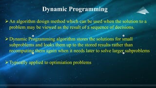
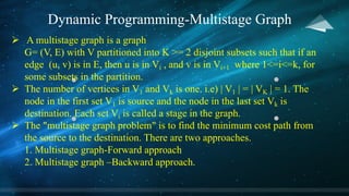
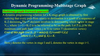
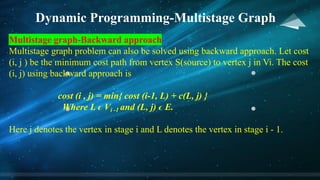
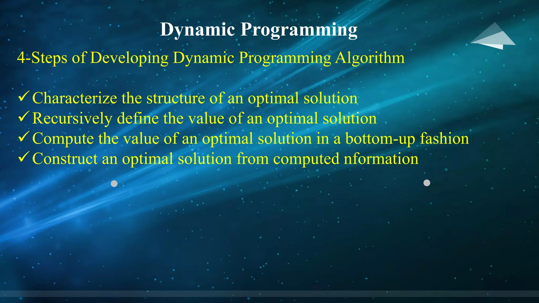
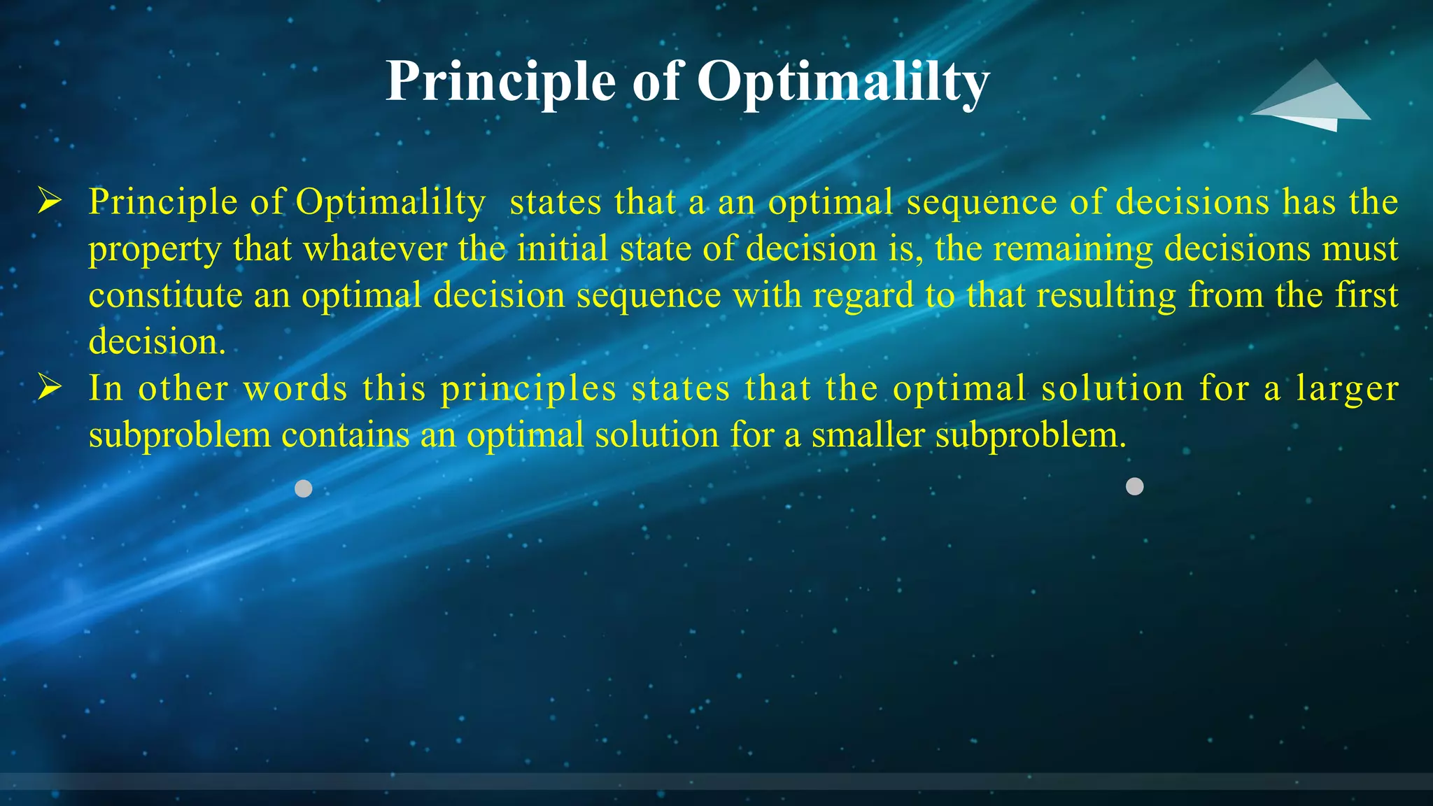
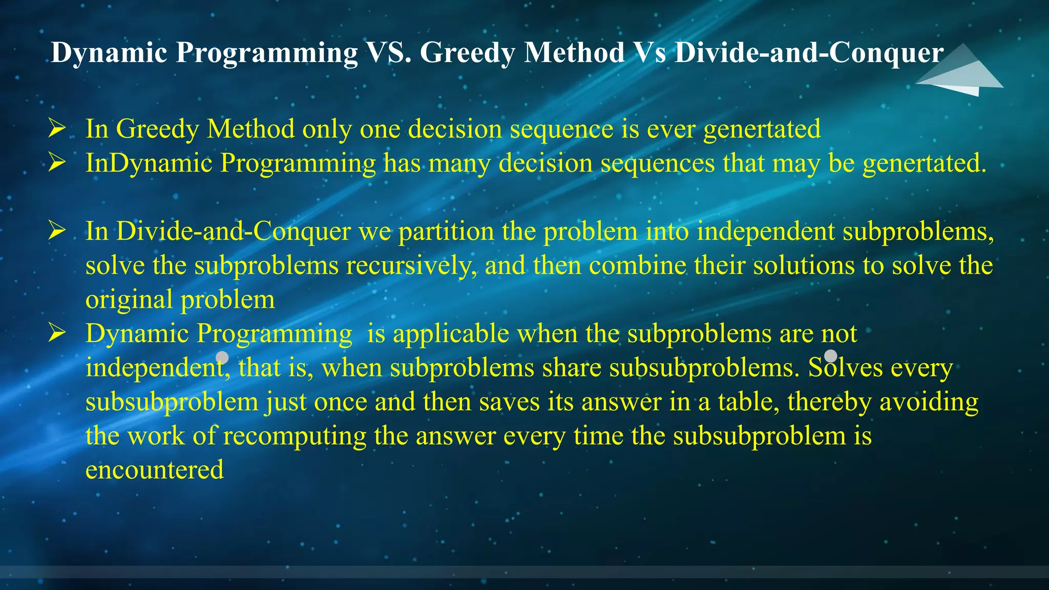
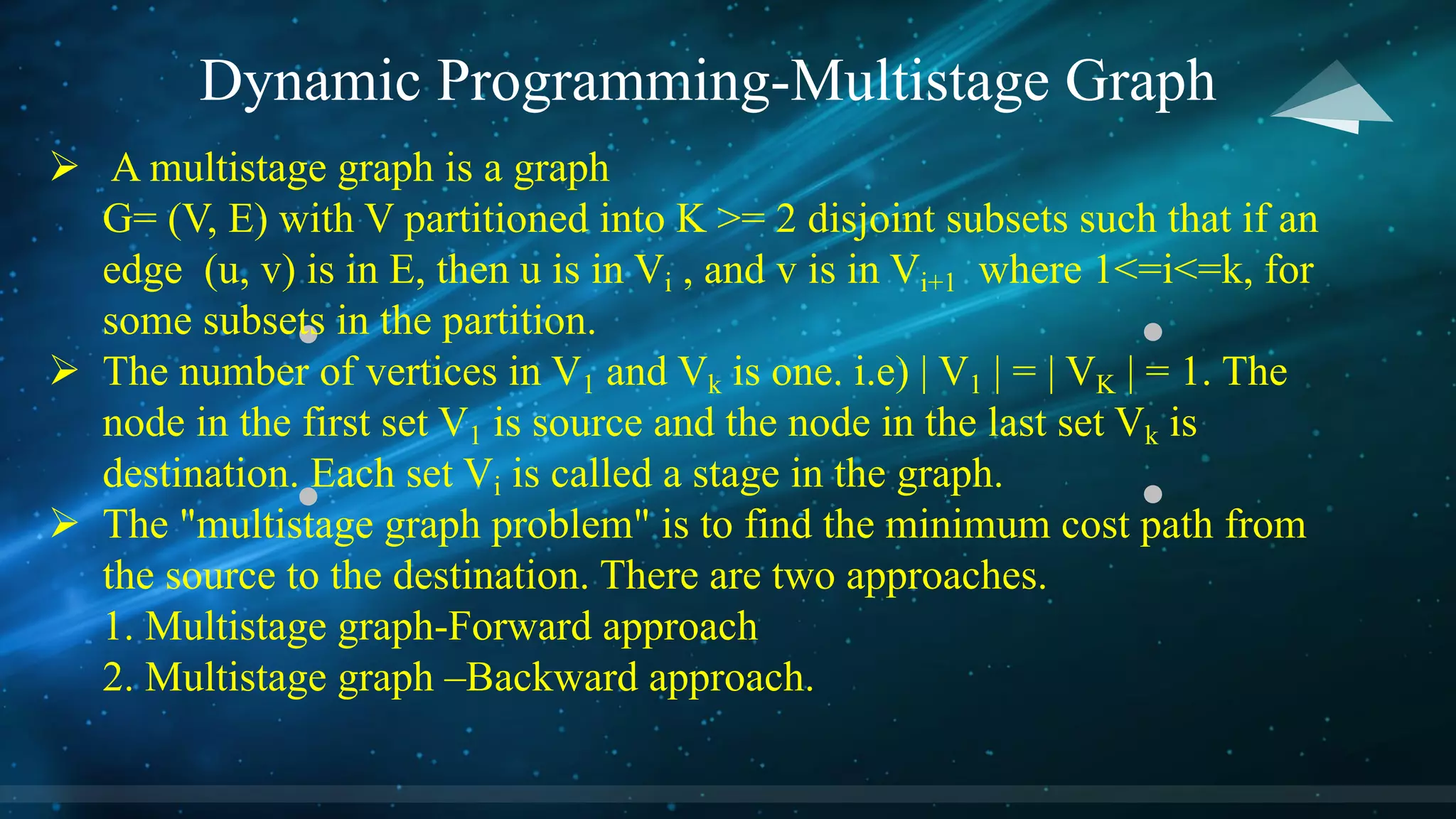
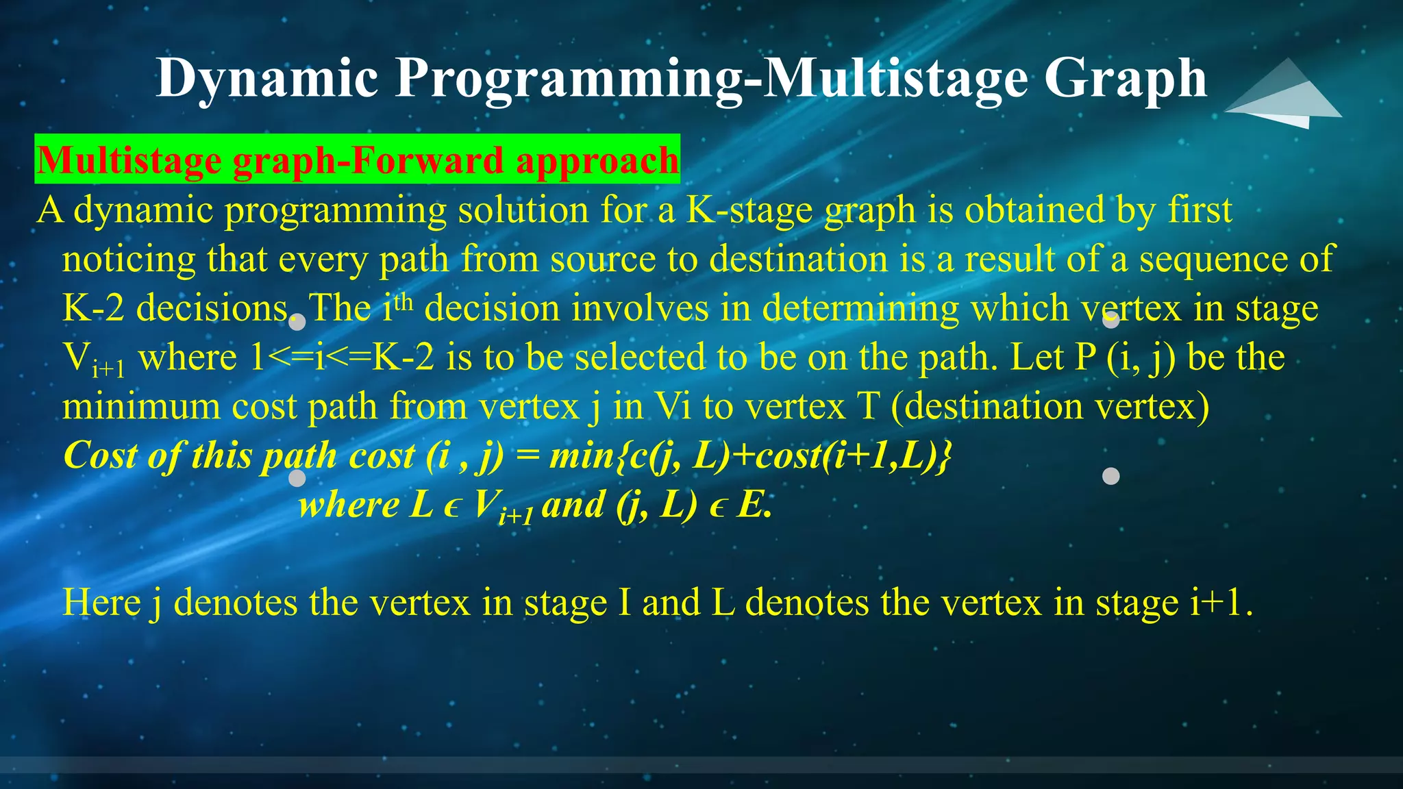
KEMBAR78
Unit 4- Dynamic Programming.pdf
UNIT 4
Dynamic Programming
Ms.Mary Jacob
Assistant Professor , Kristu Jayanti College (Autonomous),
Bangalore
Dynamic Programming
ØAn algorithm design method which can be used when the solution to a
problem may be viewed as the result of a sequence of decisions.
ØDynamic Programming algorithm stores the solutions for small
subproblems and looks them up to the stored results rather than
recomputing them again when it needs later to solve larger subproblems
ØTypically applied to optimiation problems
Dynamic Programming
4-Steps of Developing Dynamic Programming Algorithm
üCharacterize the structure of an optimal solution
üRecursively define the value of an optimal solution
üCompute the value of an optimal solution in a bottom-up fashion
üConstruct an optimal solution from computed nformation
Principle of Optimalilty
Ø Principle of Optimalilty states that a an optimal sequence of decisions has the
property that whatever the initial state of decision is, the remaining decisions must
constitute an optimal decision sequence with regard to that resulting from the first
decision.
Ø In other words this principles states that the optimal solution for a larger
subproblem contains an optimal solution for a smaller subproblem.
Dynamic Programming VS. Greedy Method Vs Divide-and-Conquer
Ø In Greedy Method only one decision sequence is ever genertated
Ø InDynamic Programming has many decision sequences that may be genertated.
Ø In Divide-and-Conquer we partition the problem into independent subproblems,
solve the subproblems recursively, and then combine their solutions to solve the
original problem
Ø Dynamic Programming is applicable when the subproblems are not
independent, that is, when subproblems share subsubproblems. Solves every
subsubproblem just once and then saves its answer in a table, thereby avoiding
the work of recomputing the answer every time the subsubproblem is
encountered
Dynamic Programming-Multistage Graph
Ø A multistage graph is a graph
G= (V, E) with V partitioned into K >= 2 disjoint subsets such that if an
edge (u, v) is in E, then u is in Vi , and v is in Vi+1 where 1<=i<=k, for
some subsets in the partition.
Ø The number of vertices in V1 and Vk is one. i.e) | V1 | = | VK | = 1. The
node in the first set V1 is source and the node in the last set Vk is
destination. Each set Vi is called a stage in the graph.
Ø The "multistage graph problem" is to find the minimum cost path from
the source to the destination. There are two approaches.
1. Multistage graph-Forward approach
2. Multistage graph –Backward approach.
Dynamic Programming-Multistage Graph
Multistage graph-Forward approach
A dynamic programming solution for a K-stage graph is obtained by first
noticing that every path from source to destination is a result of a sequence of
K-2 decisions. The ith decision involves in determining which vertex in stage
Vi+1 where 1<=i<=K-2 is to be selected to be on the path. Let P (i, j) be the
minimum cost path from vertex j in Vi to vertex T (destination vertex)
Cost of this path cost (i , j) = min{c(j, L)+cost(i+1,L)}
where L ϵ Vi+1 and (j, L) ϵ E.
Here j denotes the vertex in stage I and L denotes the vertex in stage i+1.
Dynamic Programming-Multistage Graph
Multistage graph-Backward approach
Multistage graph problem can also be solved using backward approach. Let cost
(i, j ) be the minimum cost path from vertex S(source) to vertex j in Vi. The cost
(i, j) using backward approach is
cost (i , j) = min{ cost (i-1, L) + c(L, j) }
Where L ϵ Vi -1 and (L, j) ϵ E.
Here j denotes the vertex in stage i and L denotes the vertex in stage i - 1.
All Pairs shortest Path – FLOYD Warshall Algorithm
Ø Used for solving the All Pairs Shortest Path problem.
Ø The problem is to find shortest distances between every pair of vertices in a given
edge.
Ø The solution matrix is initialized using the given graph . Then the solution matrix
is updated by considering all the vertices as an intermediate vertex.
Ø We have to pick one by one all the vertices and updates all shortest paths which
include the picked vertex as an intermediate vertex in the shortest path. When we
pick vertex number k as an intermediate vertex, we already have considered
vertices {0, 1, 2, .. k-1} as intermediate vertices. For every pair (i, j) of the source
and destination vertices, there are two possible cases1) k is not an intermediate
vertex in shortest path from i to j. We keep the value of dist[i][j] as it is2) k is an
intermediate vertex in shortest path from i to j. We update the value of dist[i][j] as
dist[i][k] + dist[k][j] if dist[i][j] > dist[i][k] + dist[k][j]
All Pairs shortest Path – FLOYD Warshall Algorithm
Formula:
Dk [i, j] =min {Dk-1[i, j], Dk-1[i, k] +Dk-1[k, j]}
Where Dk represents the matrix D after kth iteration. Initially D0=C (cost matrix). i
is the source vertex , j is the destination vertex and k represents the intermediate
vertex used.
THANK YOU

Unit 4- Dynamic Programming.pdf

  • 1.
    UNIT 4 Dynamic Programming Ms.MaryJacob Assistant Professor , Kristu Jayanti College (Autonomous), Bangalore
  • 2.
    Dynamic Programming ØAn algorithmdesign method which can be used when the solution to a problem may be viewed as the result of a sequence of decisions. ØDynamic Programming algorithm stores the solutions for small subproblems and looks them up to the stored results rather than recomputing them again when it needs later to solve larger subproblems ØTypically applied to optimiation problems
  • 3.
    Dynamic Programming 4-Steps ofDeveloping Dynamic Programming Algorithm üCharacterize the structure of an optimal solution üRecursively define the value of an optimal solution üCompute the value of an optimal solution in a bottom-up fashion üConstruct an optimal solution from computed nformation
  • 4.
    Principle of Optimalilty ØPrinciple of Optimalilty states that a an optimal sequence of decisions has the property that whatever the initial state of decision is, the remaining decisions must constitute an optimal decision sequence with regard to that resulting from the first decision. Ø In other words this principles states that the optimal solution for a larger subproblem contains an optimal solution for a smaller subproblem.
  • 5.
    Dynamic Programming VS.Greedy Method Vs Divide-and-Conquer Ø In Greedy Method only one decision sequence is ever genertated Ø InDynamic Programming has many decision sequences that may be genertated. Ø In Divide-and-Conquer we partition the problem into independent subproblems, solve the subproblems recursively, and then combine their solutions to solve the original problem Ø Dynamic Programming is applicable when the subproblems are not independent, that is, when subproblems share subsubproblems. Solves every subsubproblem just once and then saves its answer in a table, thereby avoiding the work of recomputing the answer every time the subsubproblem is encountered
  • 6.
    Dynamic Programming-Multistage Graph ØA multistage graph is a graph G= (V, E) with V partitioned into K >= 2 disjoint subsets such that if an edge (u, v) is in E, then u is in Vi , and v is in Vi+1 where 1<=i<=k, for some subsets in the partition. Ø The number of vertices in V1 and Vk is one. i.e) | V1 | = | VK | = 1. The node in the first set V1 is source and the node in the last set Vk is destination. Each set Vi is called a stage in the graph. Ø The "multistage graph problem" is to find the minimum cost path from the source to the destination. There are two approaches. 1. Multistage graph-Forward approach 2. Multistage graph –Backward approach.
  • 7.
    Dynamic Programming-Multistage Graph Multistagegraph-Forward approach A dynamic programming solution for a K-stage graph is obtained by first noticing that every path from source to destination is a result of a sequence of K-2 decisions. The ith decision involves in determining which vertex in stage Vi+1 where 1<=i<=K-2 is to be selected to be on the path. Let P (i, j) be the minimum cost path from vertex j in Vi to vertex T (destination vertex) Cost of this path cost (i , j) = min{c(j, L)+cost(i+1,L)} where L ϵ Vi+1 and (j, L) ϵ E. Here j denotes the vertex in stage I and L denotes the vertex in stage i+1.
  • 8.
    Dynamic Programming-Multistage Graph Multistagegraph-Backward approach Multistage graph problem can also be solved using backward approach. Let cost (i, j ) be the minimum cost path from vertex S(source) to vertex j in Vi. The cost (i, j) using backward approach is cost (i , j) = min{ cost (i-1, L) + c(L, j) } Where L ϵ Vi -1 and (L, j) ϵ E. Here j denotes the vertex in stage i and L denotes the vertex in stage i - 1.
  • 9.
    All Pairs shortestPath – FLOYD Warshall Algorithm Ø Used for solving the All Pairs Shortest Path problem. Ø The problem is to find shortest distances between every pair of vertices in a given edge. Ø The solution matrix is initialized using the given graph . Then the solution matrix is updated by considering all the vertices as an intermediate vertex. Ø We have to pick one by one all the vertices and updates all shortest paths which include the picked vertex as an intermediate vertex in the shortest path. When we pick vertex number k as an intermediate vertex, we already have considered vertices {0, 1, 2, .. k-1} as intermediate vertices. For every pair (i, j) of the source and destination vertices, there are two possible cases1) k is not an intermediate vertex in shortest path from i to j. We keep the value of dist[i][j] as it is2) k is an intermediate vertex in shortest path from i to j. We update the value of dist[i][j] as dist[i][k] + dist[k][j] if dist[i][j] > dist[i][k] + dist[k][j]
  • 10.
    All Pairs shortestPath – FLOYD Warshall Algorithm Formula: Dk [i, j] =min {Dk-1[i, j], Dk-1[i, k] +Dk-1[k, j]} Where Dk represents the matrix D after kth iteration. Initially D0=C (cost matrix). i is the source vertex , j is the destination vertex and k represents the intermediate vertex used.
  • 11.