Download as PDF, PPTX

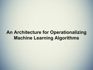


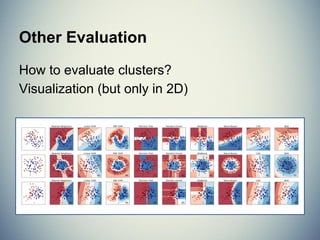


![MSE & Coefficient of Determination
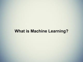
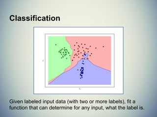
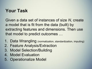
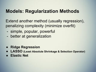
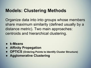
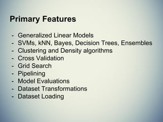
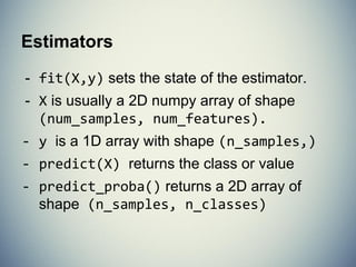
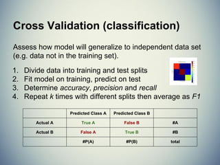
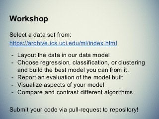
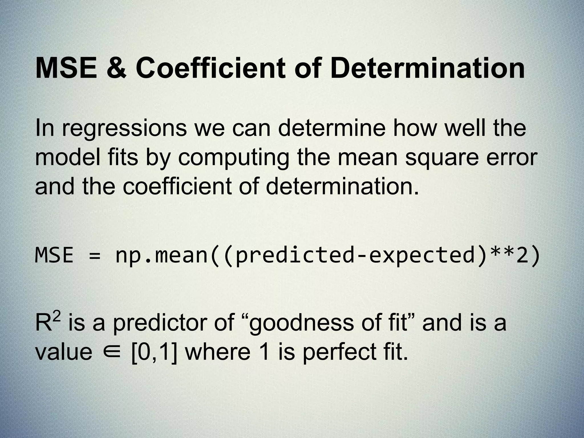
In regressions we can determine how well the
model fits by computing the mean square error
and the coefficient of determination.
MSE = np.mean((predicted-expected)**2)
R2
is a predictor of “goodness of fit” and is a
value ∈ [0,1] where 1 is perfect fit.](https://image.slidesharecdn.com/introductiontomachinelearningwithscikit-learn-150227223526-conversion-gate01/85/Introduction-to-Machine-Learning-with-SciKit-Learn-60-320.jpg)


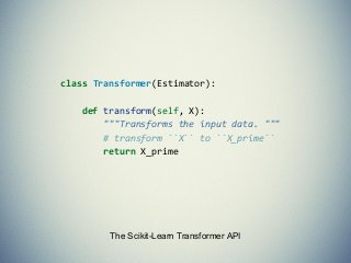
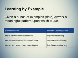
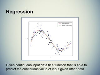
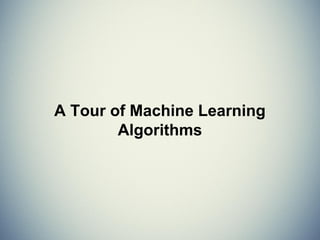
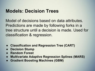
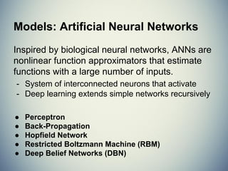
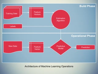
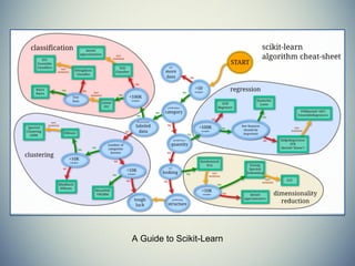
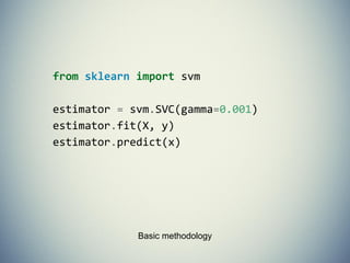
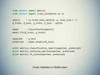
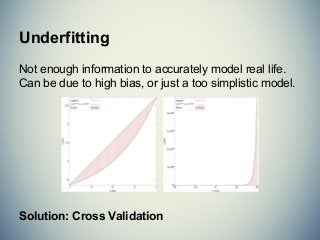
![Pipelined Model
>>> from sklearn.preprocessing import PolynomialFeatures
>>> from sklearn.pipeline import make_pipeline
>>> model = make_pipeline(PolynomialFeatures(2), linear_model.
Ridge())
>>> model.fit(X_train, y_train)
Pipeline(steps=[('polynomialfeatures', PolynomialFeatures(degree=2,
include_bias=True, interaction_only=False)), ('ridge', Ridge
(alpha=1.0, copy_X=True, fit_intercept=True, max_iter=None,
normalize=False, solver='auto', tol=0.001))])
>>> mean_squared_error(y_test, model.predict(X_test))
3.1498887586451594
>>> model.score(X_test, y_test)
0.97090576345108104](https://image.slidesharecdn.com/introductiontomachinelearningwithscikit-learn-150227223526-conversion-gate01/85/Introduction-to-Machine-Learning-with-SciKit-Learn-72-320.jpg)

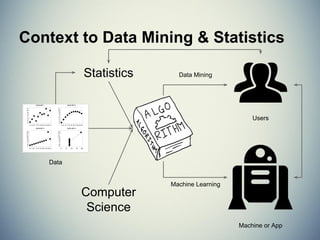
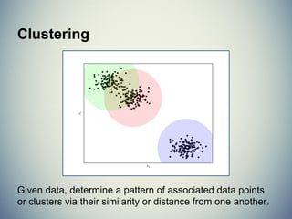
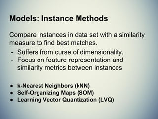
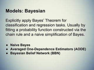
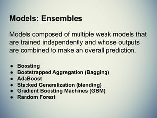
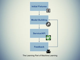
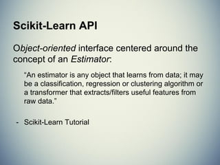
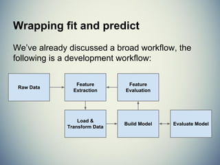
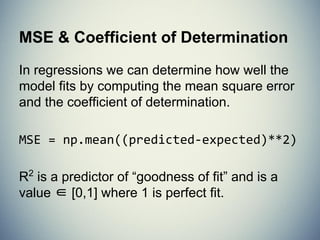
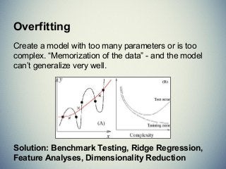
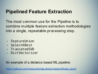
![Error as a function of alpha
>>> clf = linear_model.Ridge(fit_intercept=False)
>>> errors = []
>>> for alpha in alphas:
... splits = tts(dataset.data, dataset.target('Y1'), test_size=0.2)
... X_train, X_test, y_train, y_test = splits
... clf.set_params(alpha=alpha)
... clf.fit(X_train, y_train)
... error = mean_squared_error(y_test, clf.predict(X_test))
... errors.append(error)
...
>>> axe = plt.gca()
>>> axe.plot(alphas, errors)
>>> plt.show()](https://image.slidesharecdn.com/introductiontomachinelearningwithscikit-learn-150227223526-conversion-gate01/85/Introduction-to-Machine-Learning-with-SciKit-Learn-77-320.jpg)


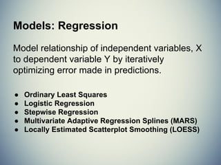
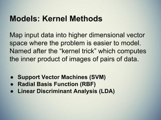
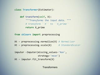
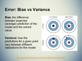
![MSE & Coefficient of Determination
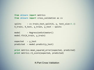
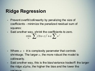
In regressions we can determine how well the
model fits by computing the mean square error
and the coefficient of determination.
MSE = np.mean((predicted-expected)**2)
R2
is a predictor of “goodness of fit” and is a
value ∈ [0,1] where 1 is perfect fit.](https://image.slidesharecdn.com/introductiontomachinelearningwithscikit-learn-150227223526-conversion-gate01/75/Introduction-to-Machine-Learning-with-SciKit-Learn-60-2048.jpg)


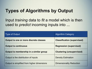
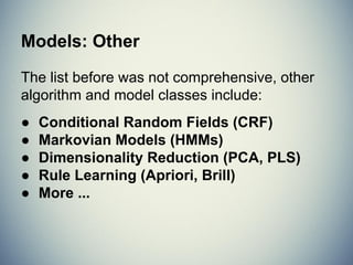
![Pipelined Model
>>> from sklearn.preprocessing import PolynomialFeatures
>>> from sklearn.pipeline import make_pipeline
>>> model = make_pipeline(PolynomialFeatures(2), linear_model.
Ridge())
>>> model.fit(X_train, y_train)
Pipeline(steps=[('polynomialfeatures', PolynomialFeatures(degree=2,
include_bias=True, interaction_only=False)), ('ridge', Ridge
(alpha=1.0, copy_X=True, fit_intercept=True, max_iter=None,
normalize=False, solver='auto', tol=0.001))])
>>> mean_squared_error(y_test, model.predict(X_test))
3.1498887586451594
>>> model.score(X_test, y_test)
0.97090576345108104](https://image.slidesharecdn.com/introductiontomachinelearningwithscikit-learn-150227223526-conversion-gate01/75/Introduction-to-Machine-Learning-with-SciKit-Learn-72-2048.jpg)


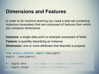
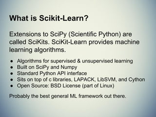
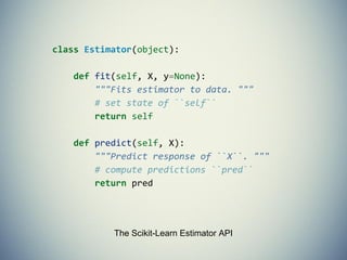
![Error as a function of alpha
>>> clf = linear_model.Ridge(fit_intercept=False)
>>> errors = []
>>> for alpha in alphas:
... splits = tts(dataset.data, dataset.target('Y1'), test_size=0.2)
... X_train, X_test, y_train, y_test = splits
... clf.set_params(alpha=alpha)
... clf.fit(X_train, y_train)
... error = mean_squared_error(y_test, clf.predict(X_test))
... errors.append(error)
...
>>> axe = plt.gca()
>>> axe.plot(alphas, errors)
>>> plt.show()](https://image.slidesharecdn.com/introductiontomachinelearningwithscikit-learn-150227223526-conversion-gate01/75/Introduction-to-Machine-Learning-with-SciKit-Learn-77-2048.jpg)


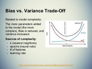
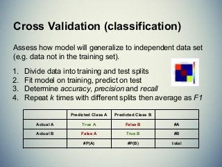
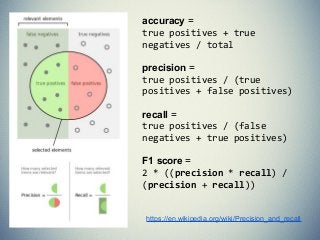
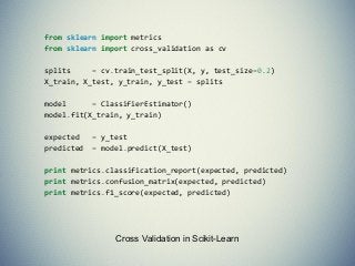
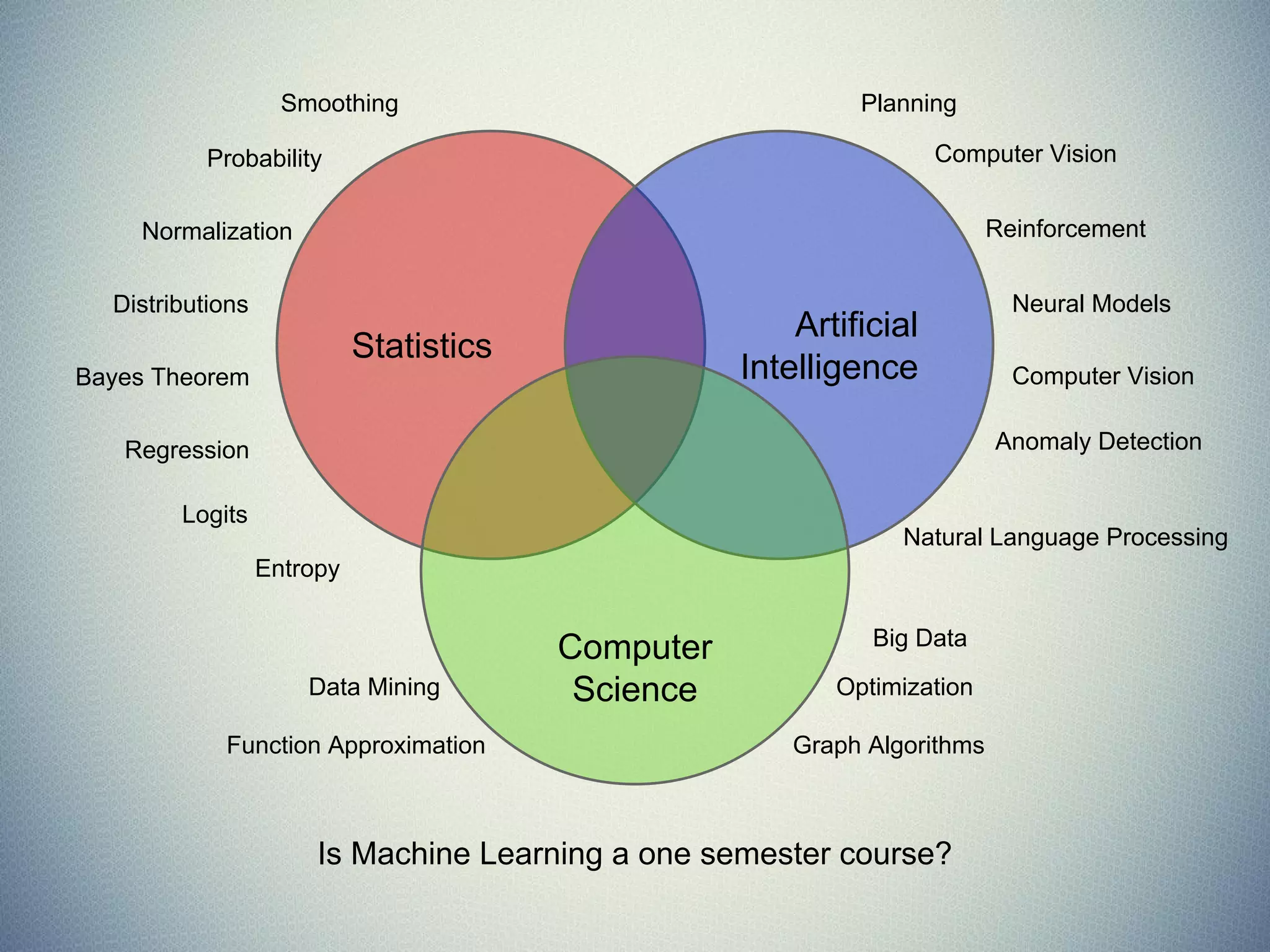
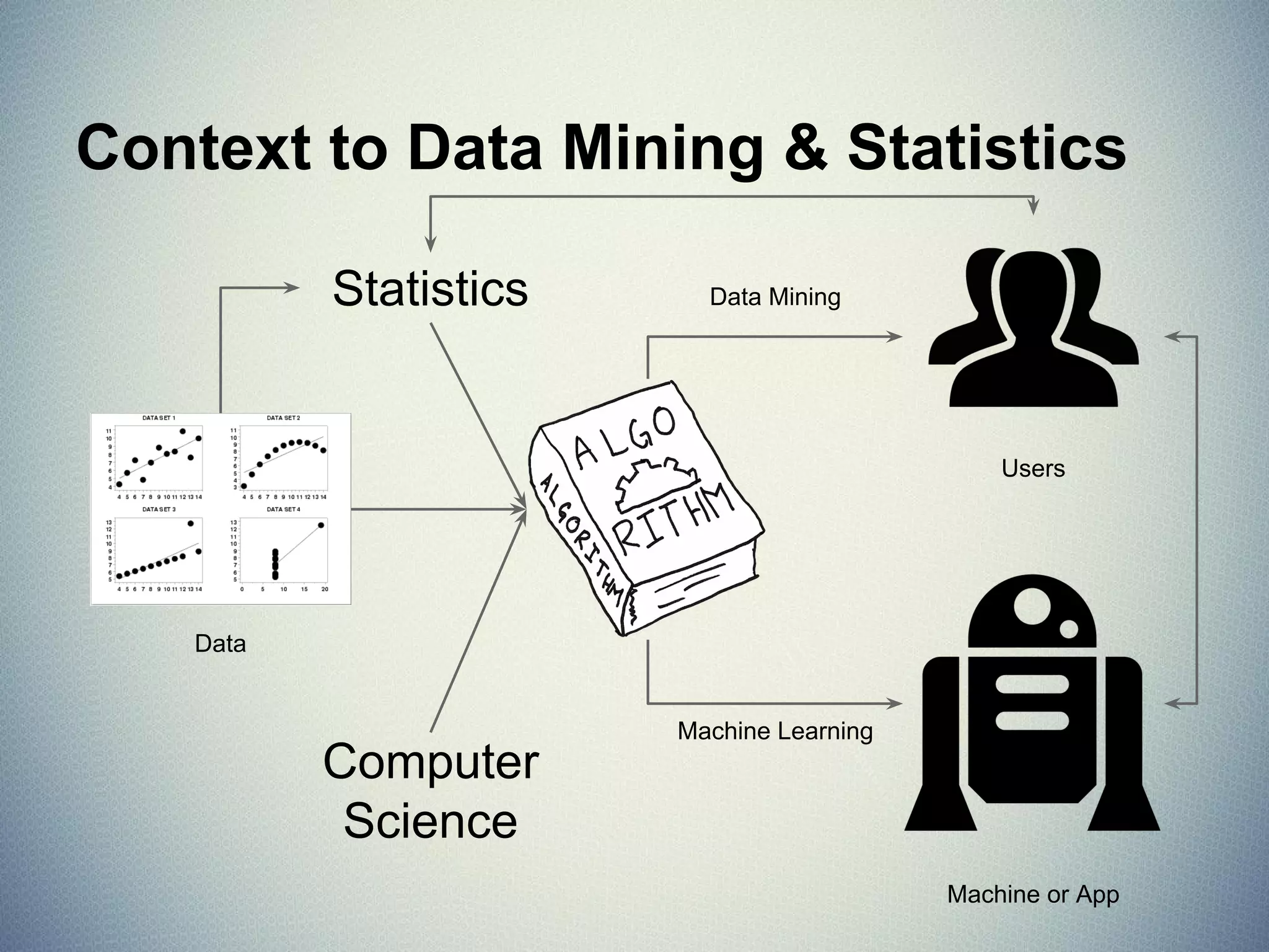
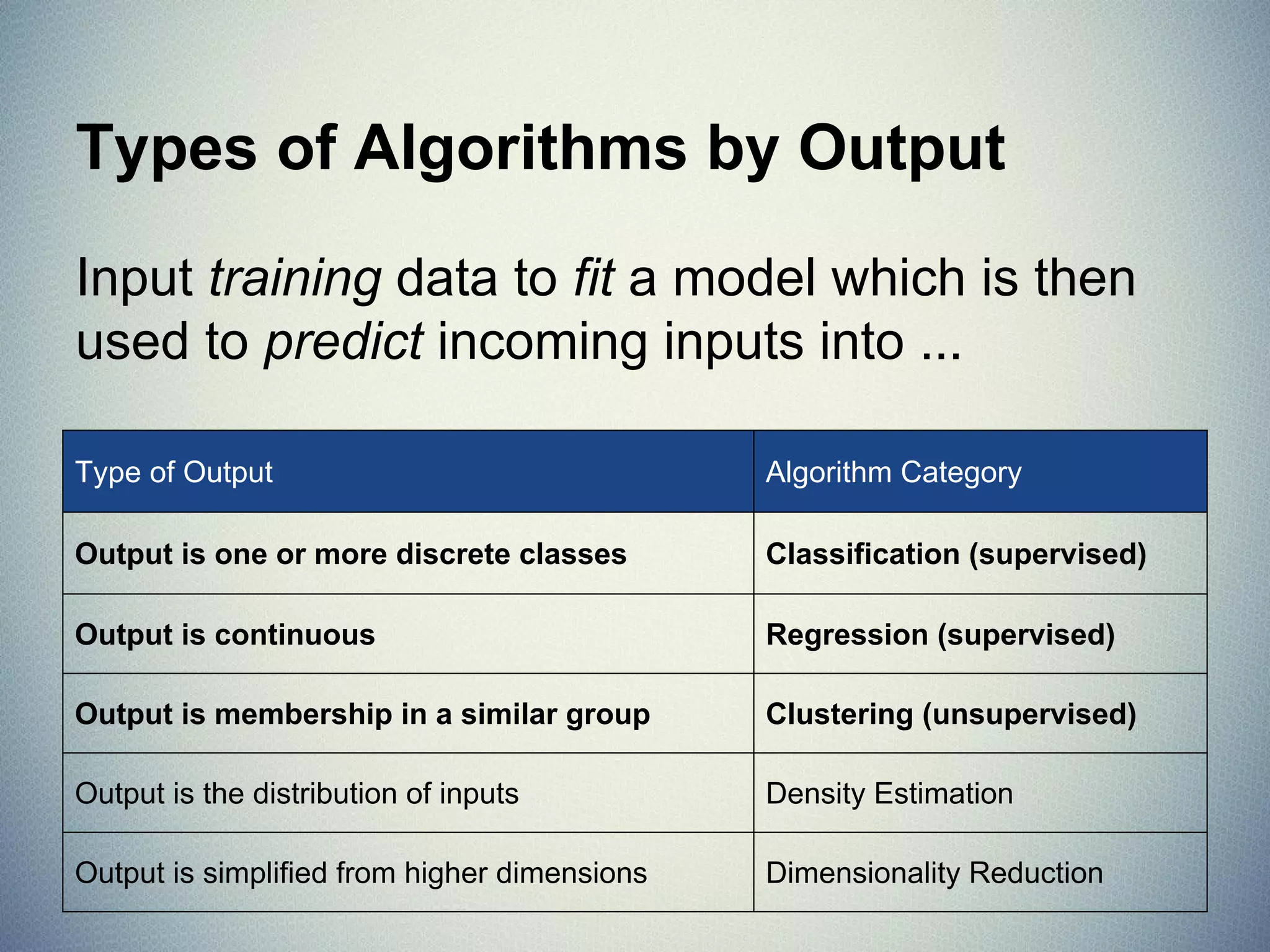
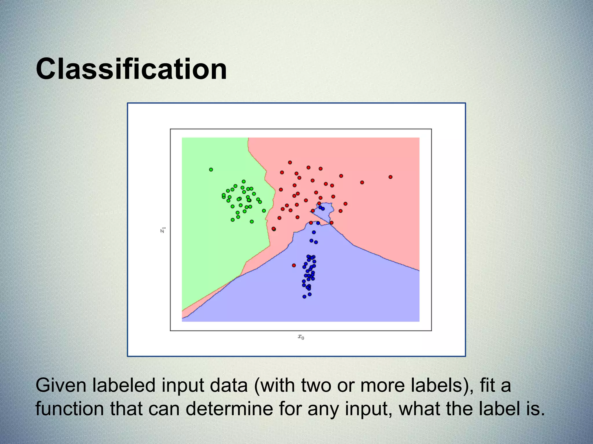
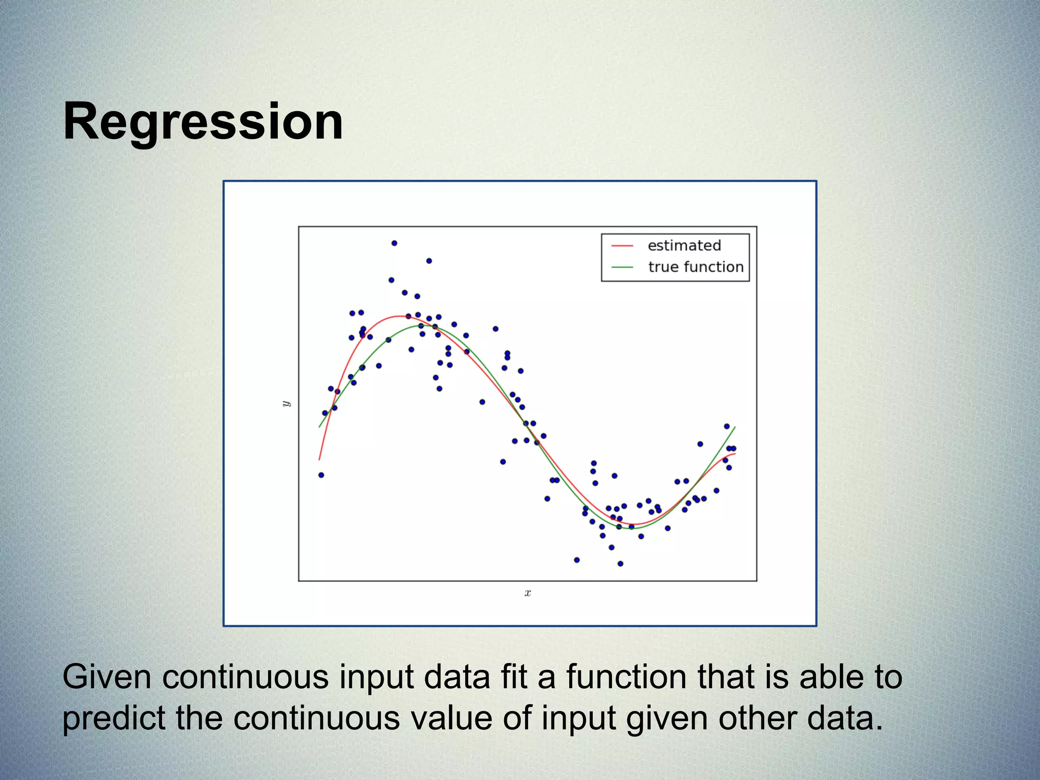
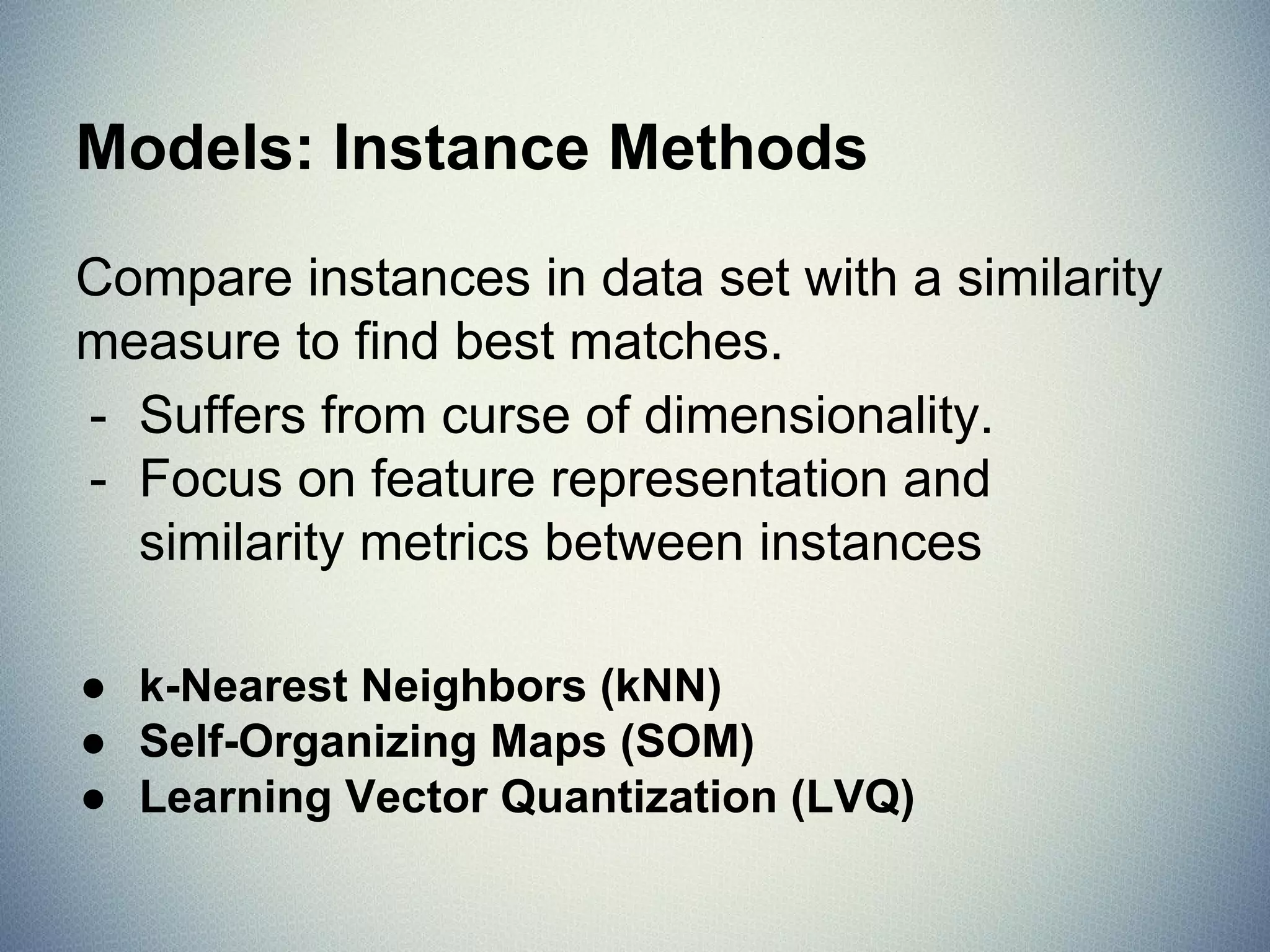
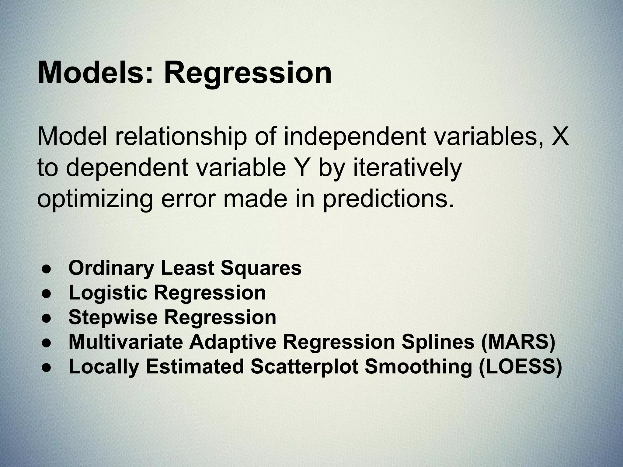
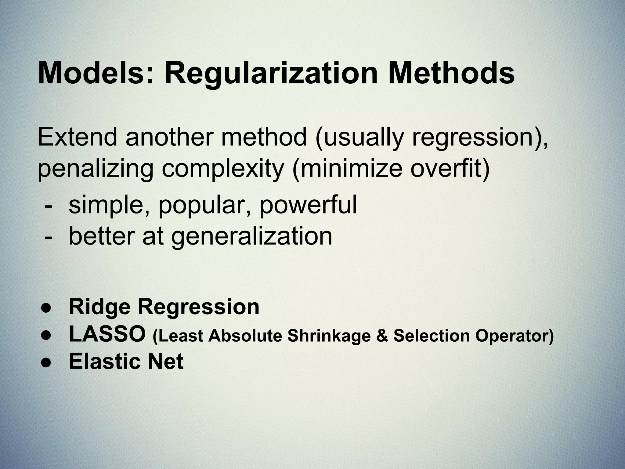
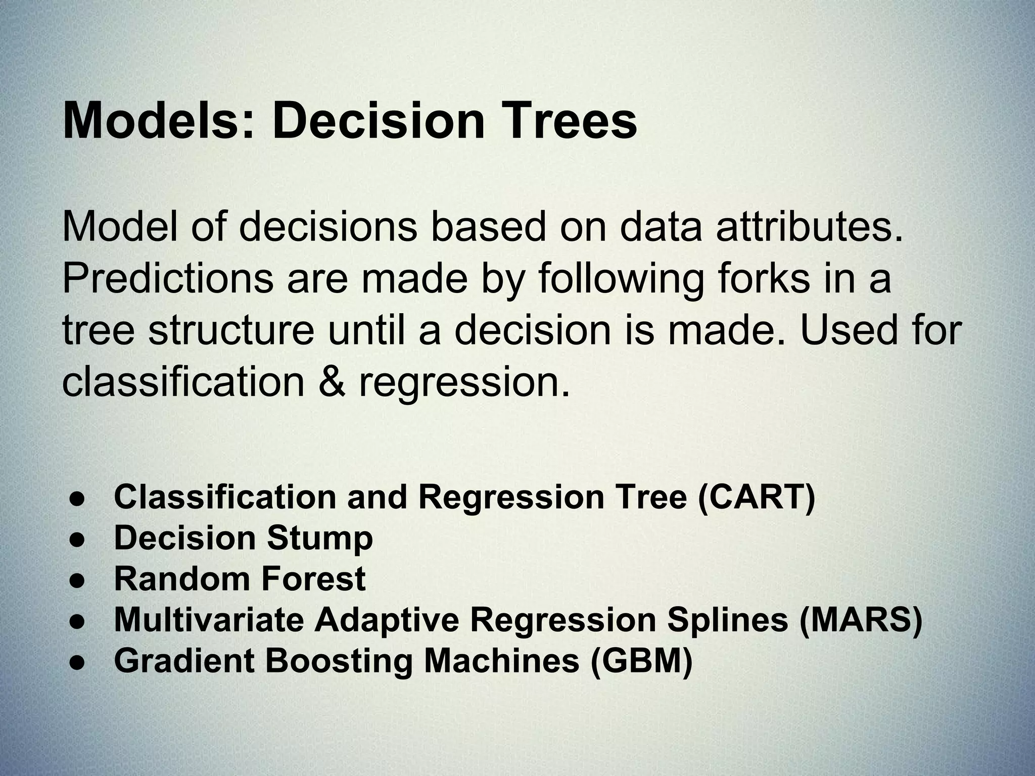
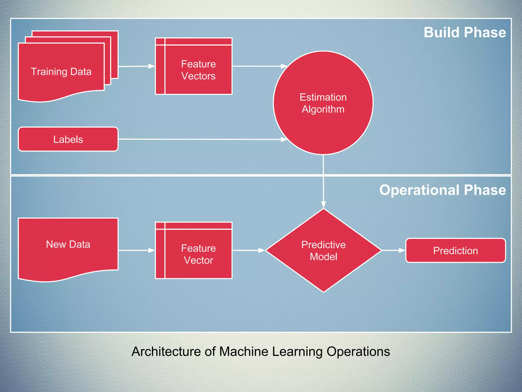
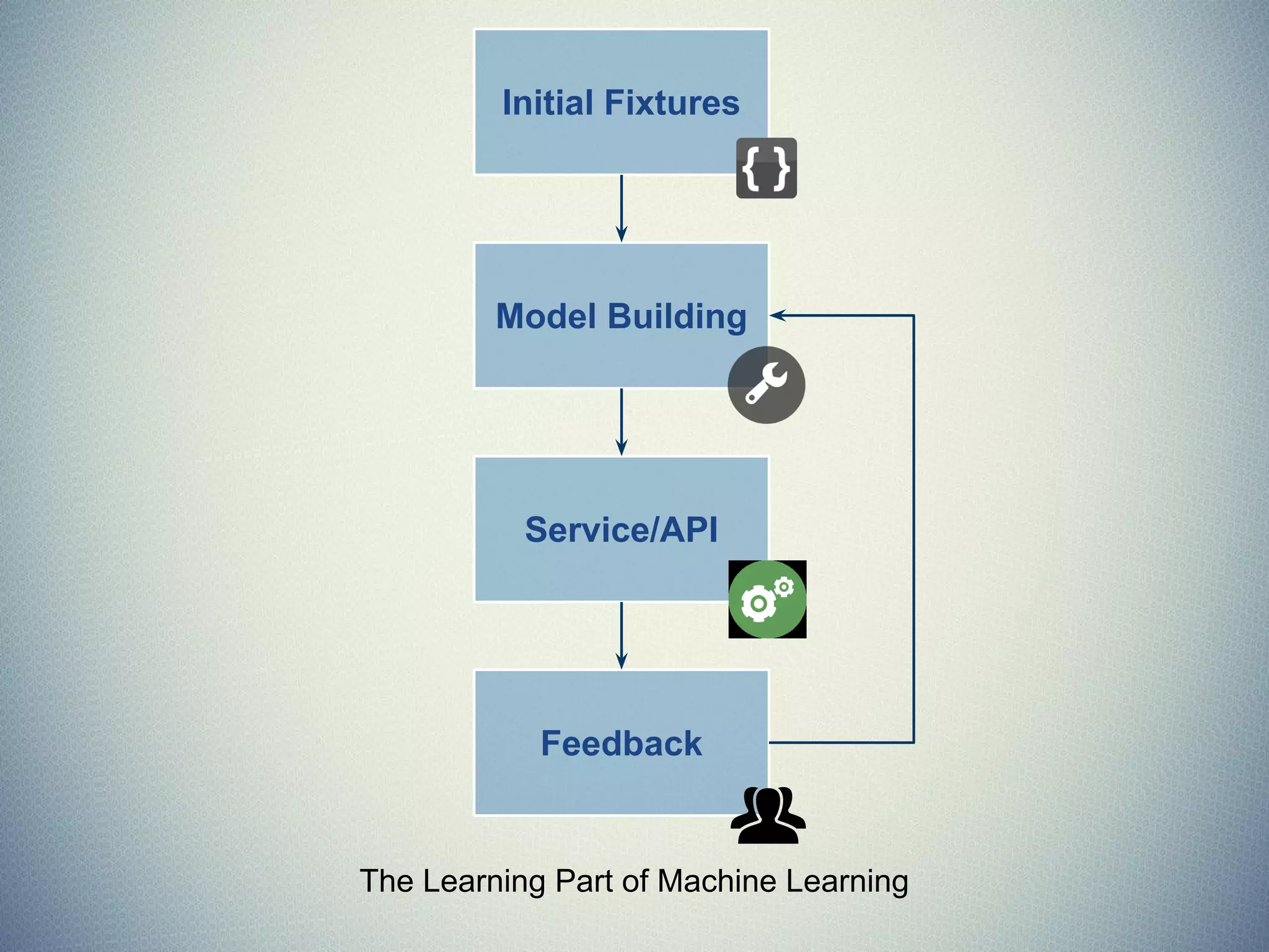
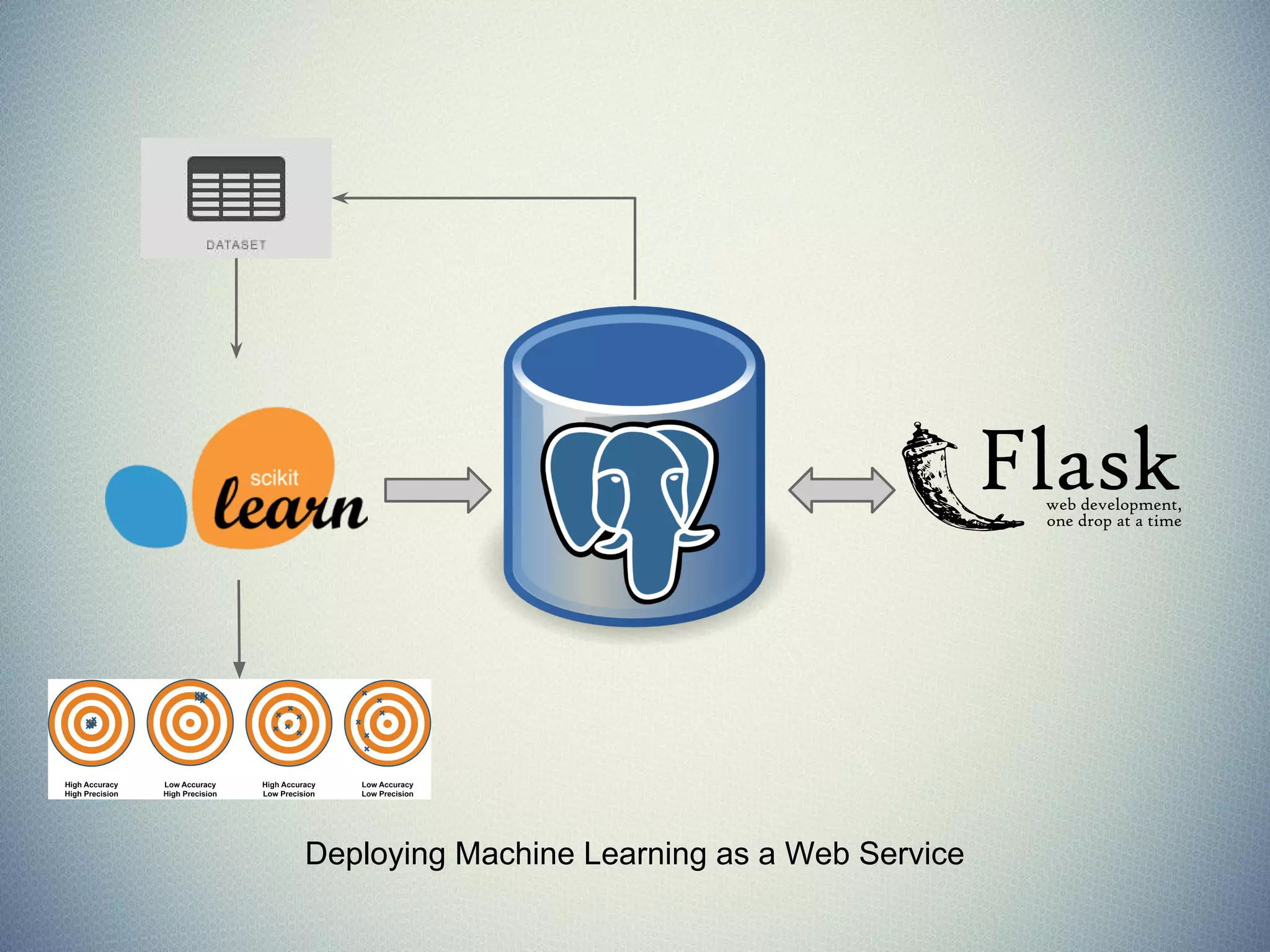
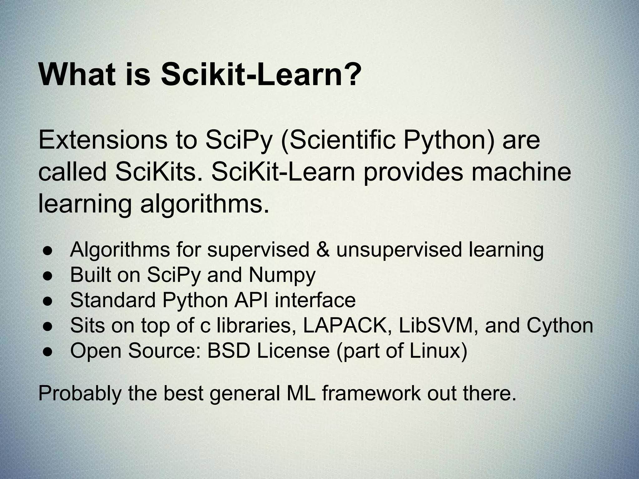
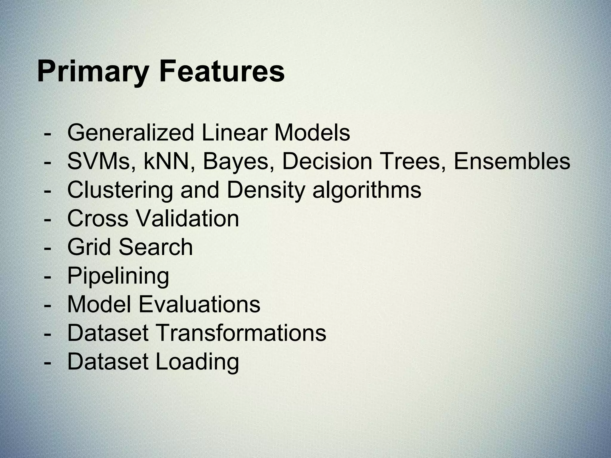
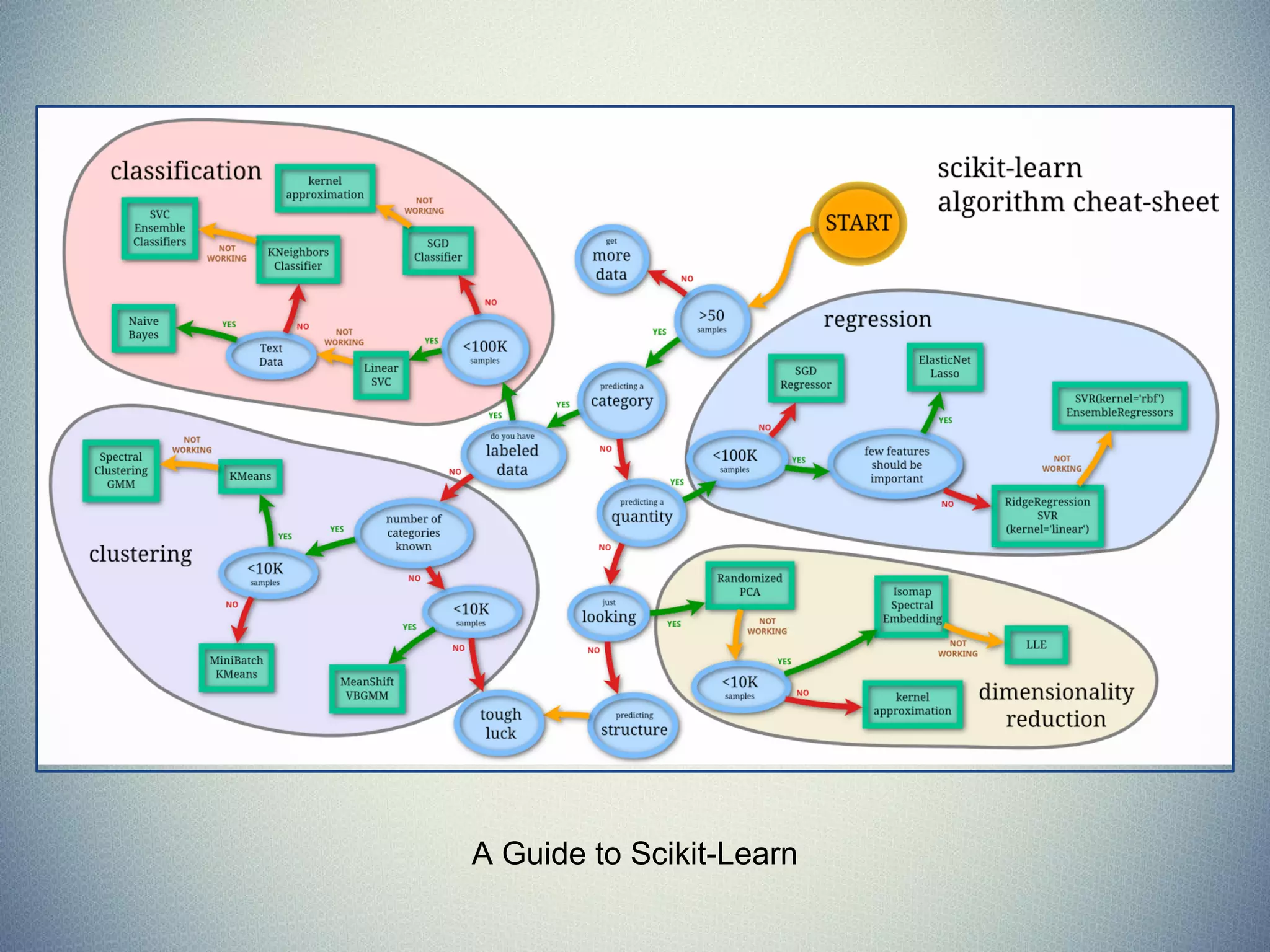
The document provides an extensive overview of machine learning concepts, particularly using the scikit-learn library, covering topics such as supervised and unsupervised learning, model evaluation, and various algorithms. It outlines the process of building machine learning models, including data handling, feature extraction, and evaluation metrics, as well as discussing the architecture for operationalizing these models. Additionally, it introduces scikit-learn, its features, and the importance of proper methodology to avoid overfitting and underfitting in machine learning applications.


