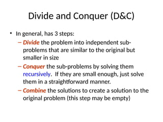
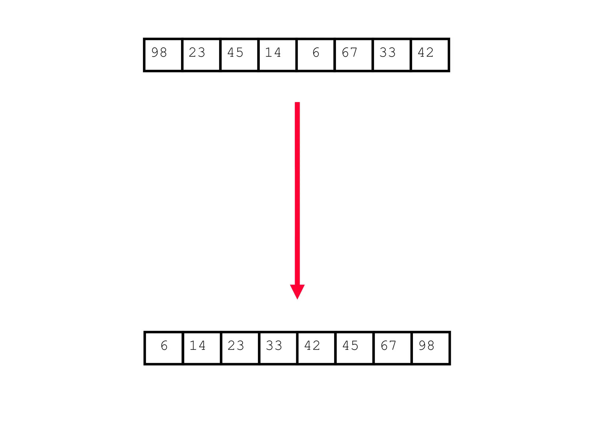
The document discusses divide and conquer algorithms, focusing on binary search and merge sort. It explains the recursive steps of the binary search algorithm to locate an item in a sorted array and the merge sort process for sorting a sequence of elements. The time complexity for binary search is given as θ(lg n), and for merge sort, the overall time complexity is θ(n).

![A motivating Example of D&C Algorithm
Binary Search (recursive)
// Returns location of x in the sorted array A[first..last] if x is in A, otherwise returns -1
Algorithm BinarySearch(A, first, last, x)
if last ≥ first then
mid = first + (last - first)/2
// If the element is present at the middle itself
if A[mid] = x then
return mid
// If element is smaller than mid, then it can only be present in left sub-array
else if A[mid] > x then
return BinarySearch(A, first, mid-1, x)
// Otherwise the element can only be present in the right sub-array
else
return BinarySearch(A, mid+1, last, x);
Initial call: BinarySearch(A,1,n,key) where key is an user input which is to be sought in A](https://image.slidesharecdn.com/l2divideconquer-241117011201-6376395f/85/L2_DatabAlgorithm-Basics-with-Design-Analysis-pptx-2-320.jpg)

![Binary Search (recursive) Algorithm
// Returns location of x in the sorted array A[first..last] if x is in A, otherwise returns -1
Algorithm BinarySearch(A, p, q, x)
if last ≥ first then
mid (p+q)/2
// If the element is present at the middle itself
if A[mid] = x then
return mid
// If element is smaller than mid, then it can only be present in left sub-array
if A[mid] > x then
return BinarySearch(A, p, mid-1, x)
// Otherwise the element can only be present in the right sub-array
else
return BinarySearch(A, mid+1, q, x)
return -1 // We reach here when element is not present in A
Initial call: BinarySearch(A,1,n,key) where key is an user input which is to be sought in A
Time: Θ(lg n), why?](https://image.slidesharecdn.com/l2divideconquer-241117011201-6376395f/85/L2_DatabAlgorithm-Basics-with-Design-Analysis-pptx-15-320.jpg)
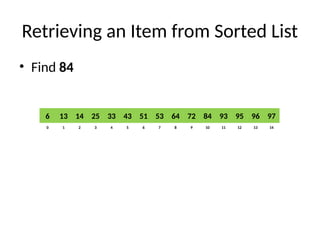
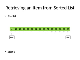
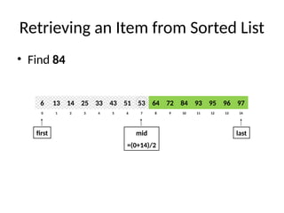
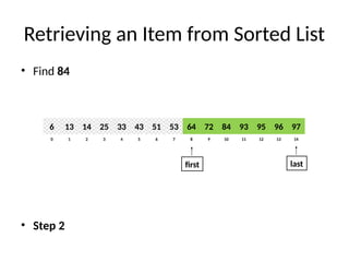
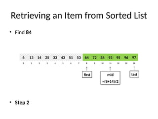
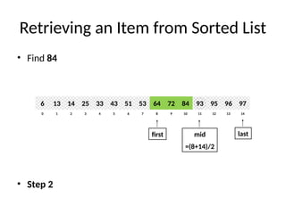
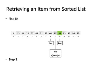
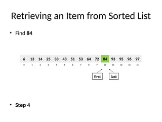
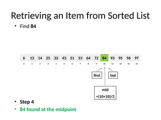
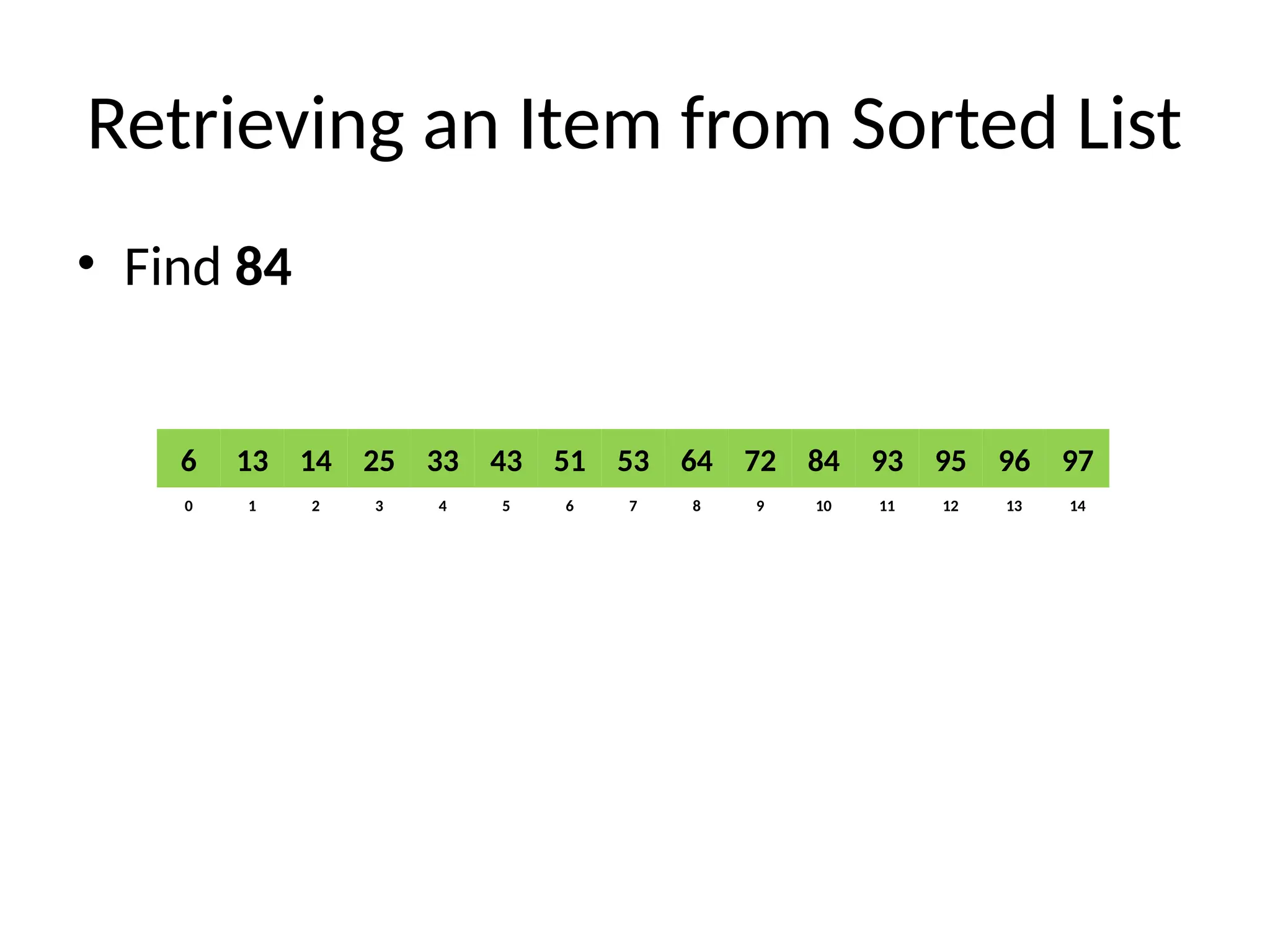
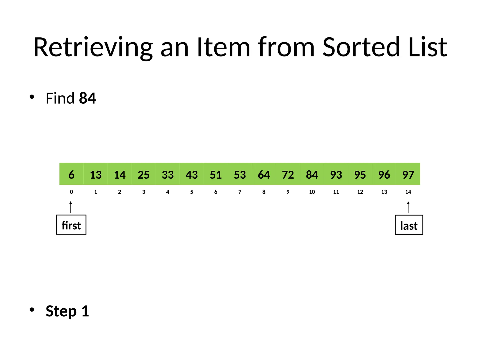
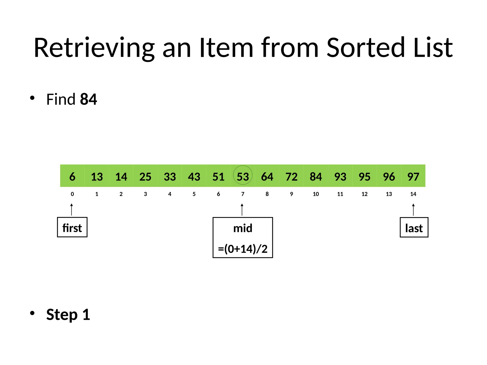
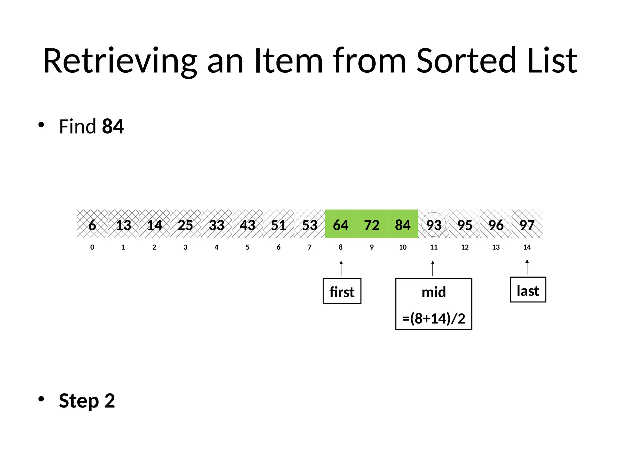
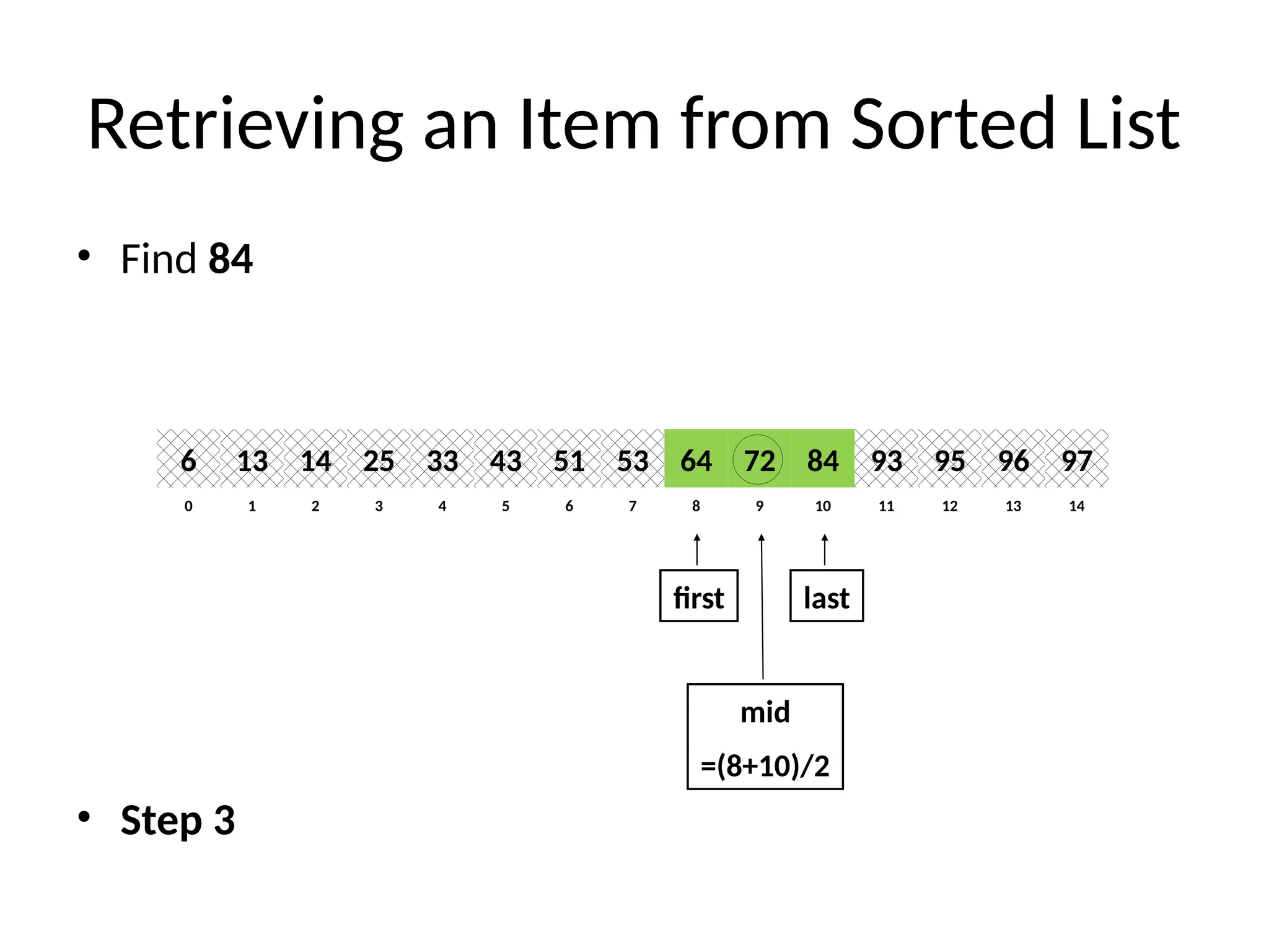
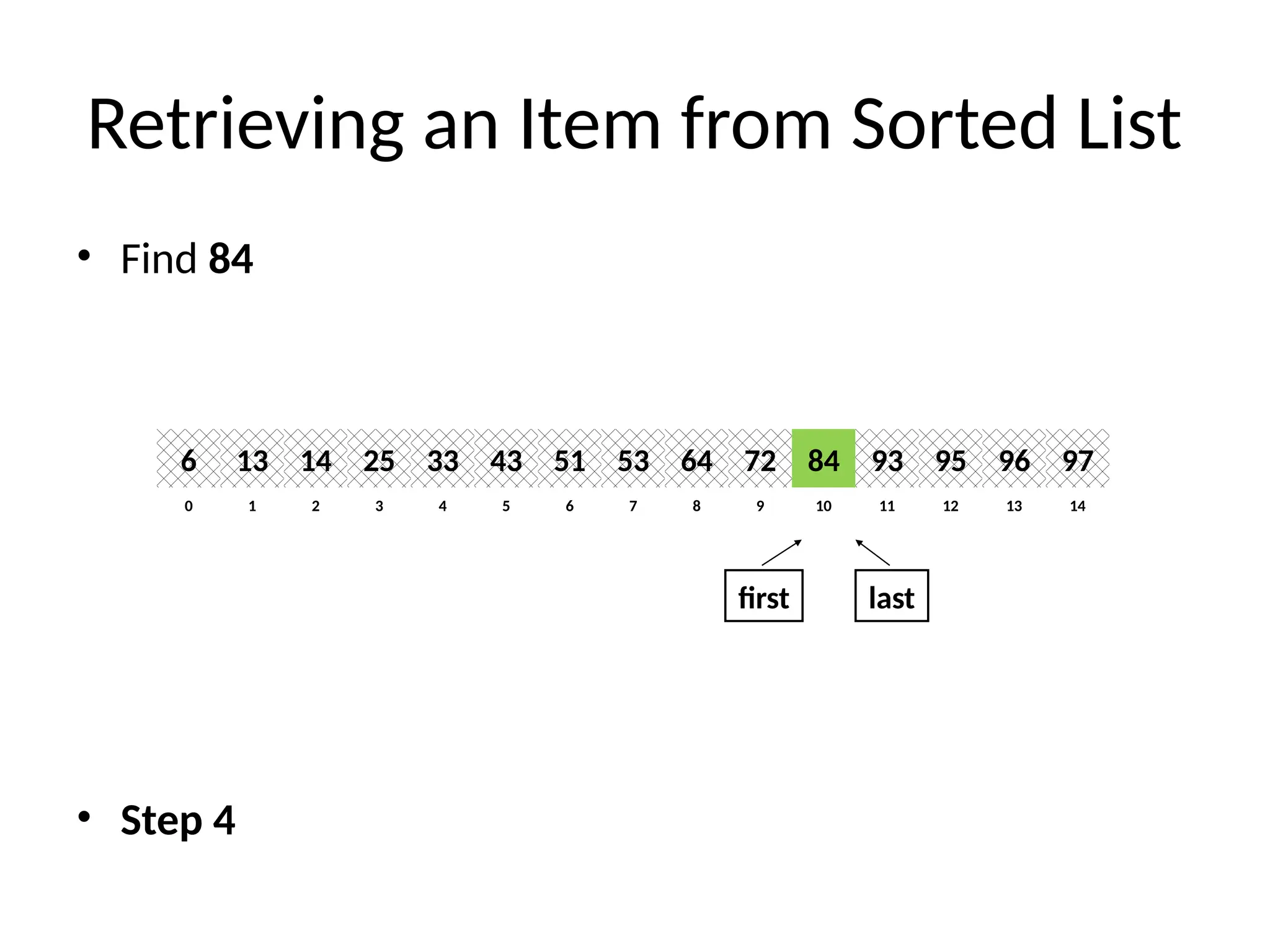
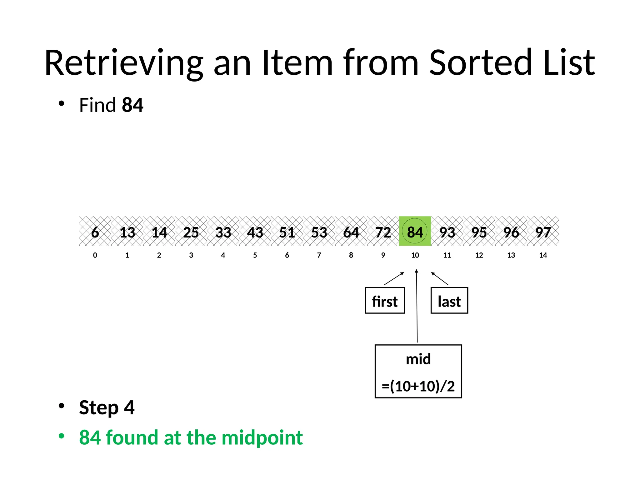
![D&C Algorithm Example: Binary Search
Searching Problem: Search for item in a sorted sequence A of n elements
Divide: Divide the n-element input array into two subarray of ≈ n/2 elements
each:
m (p+q)/2
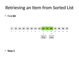
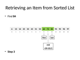
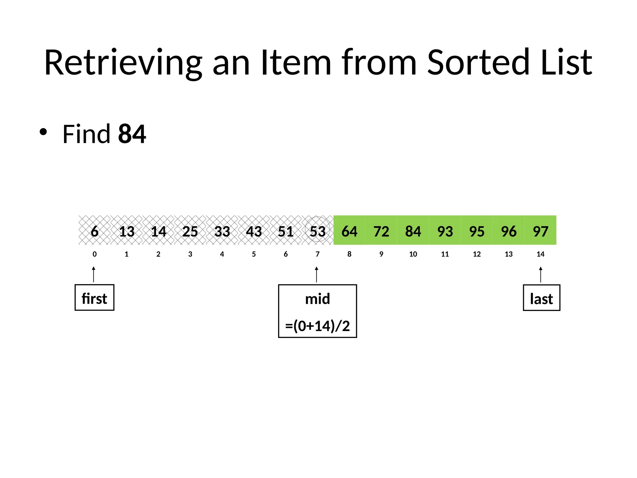
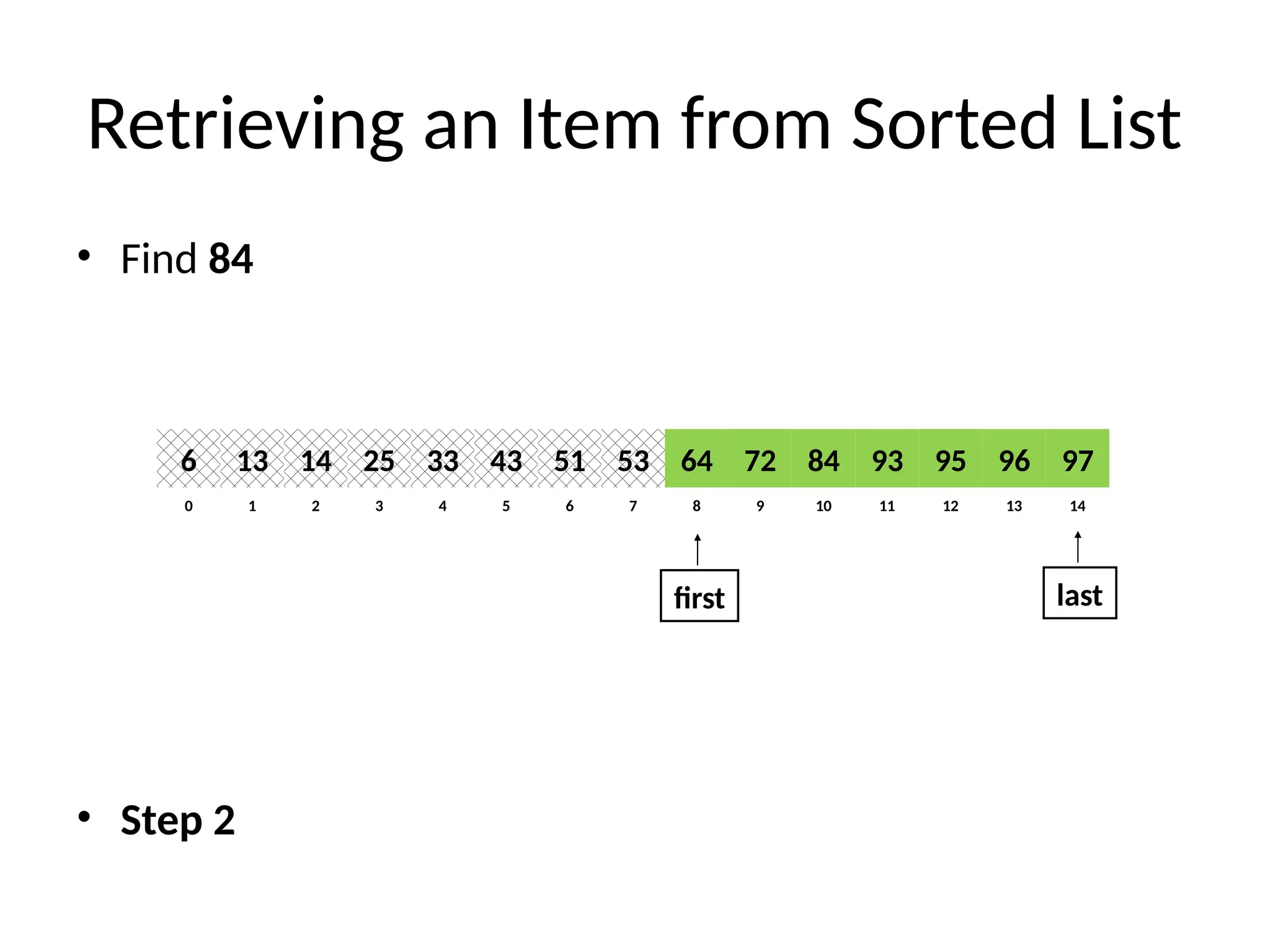
Conquer: Search either of the subarrays recursively by calling BinarySearch on
the appropriate subarray:
if A[m] > x then
return BinarySearch(A, p, m-1, x)
else
return BinarySearch(A, m+1, q, x)
Combine: Nothing to be done](https://image.slidesharecdn.com/l2divideconquer-241117011201-6376395f/85/L2_DatabAlgorithm-Basics-with-Design-Analysis-pptx-17-320.jpg)
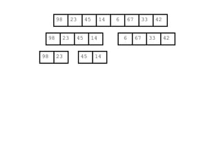
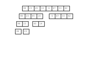
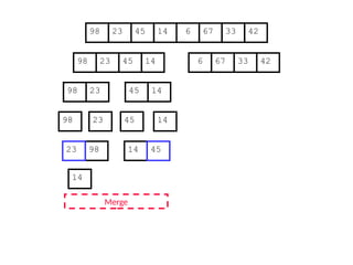
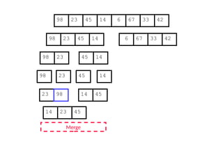
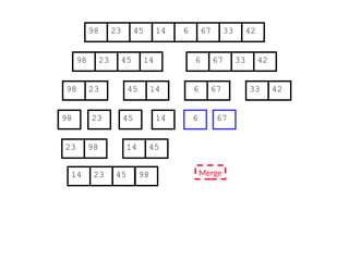
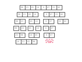
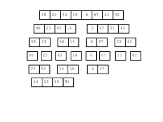
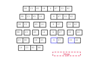
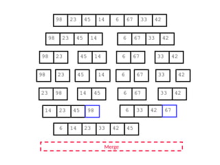
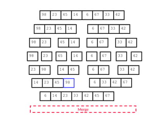
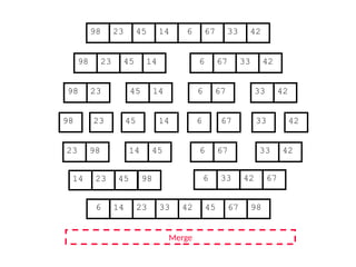
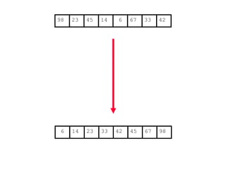
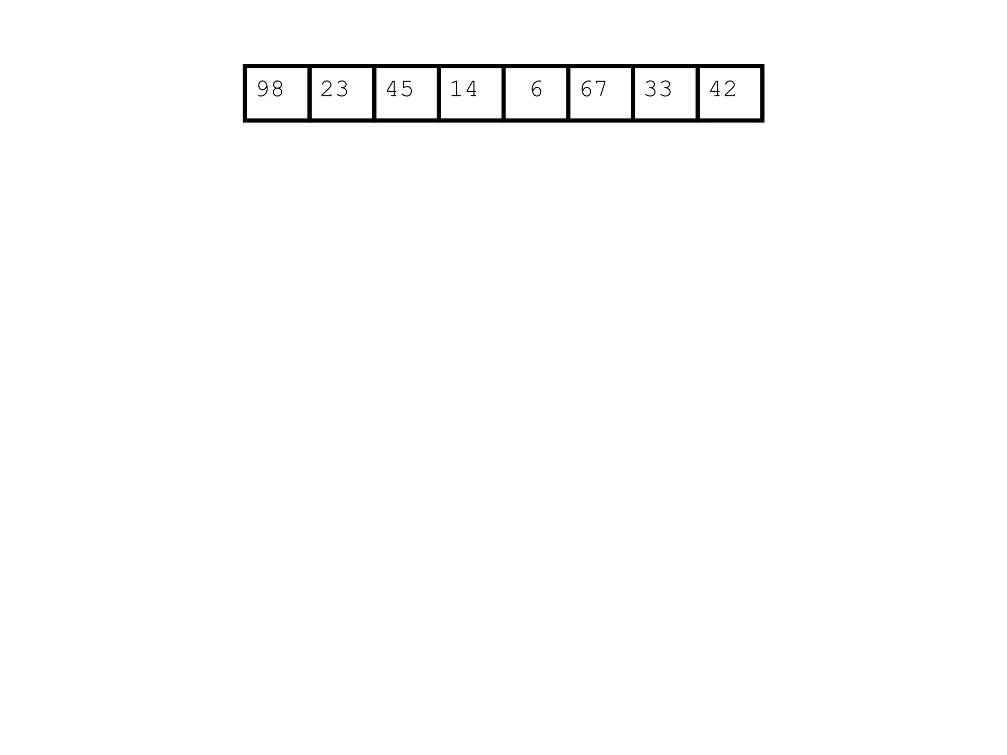
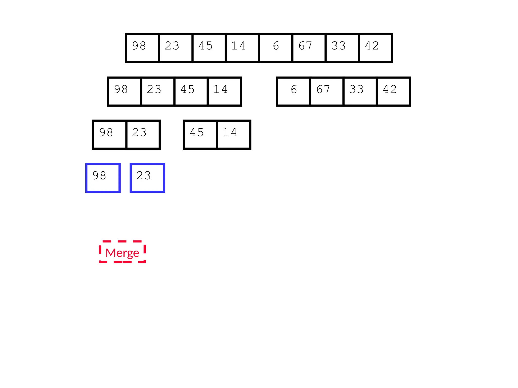
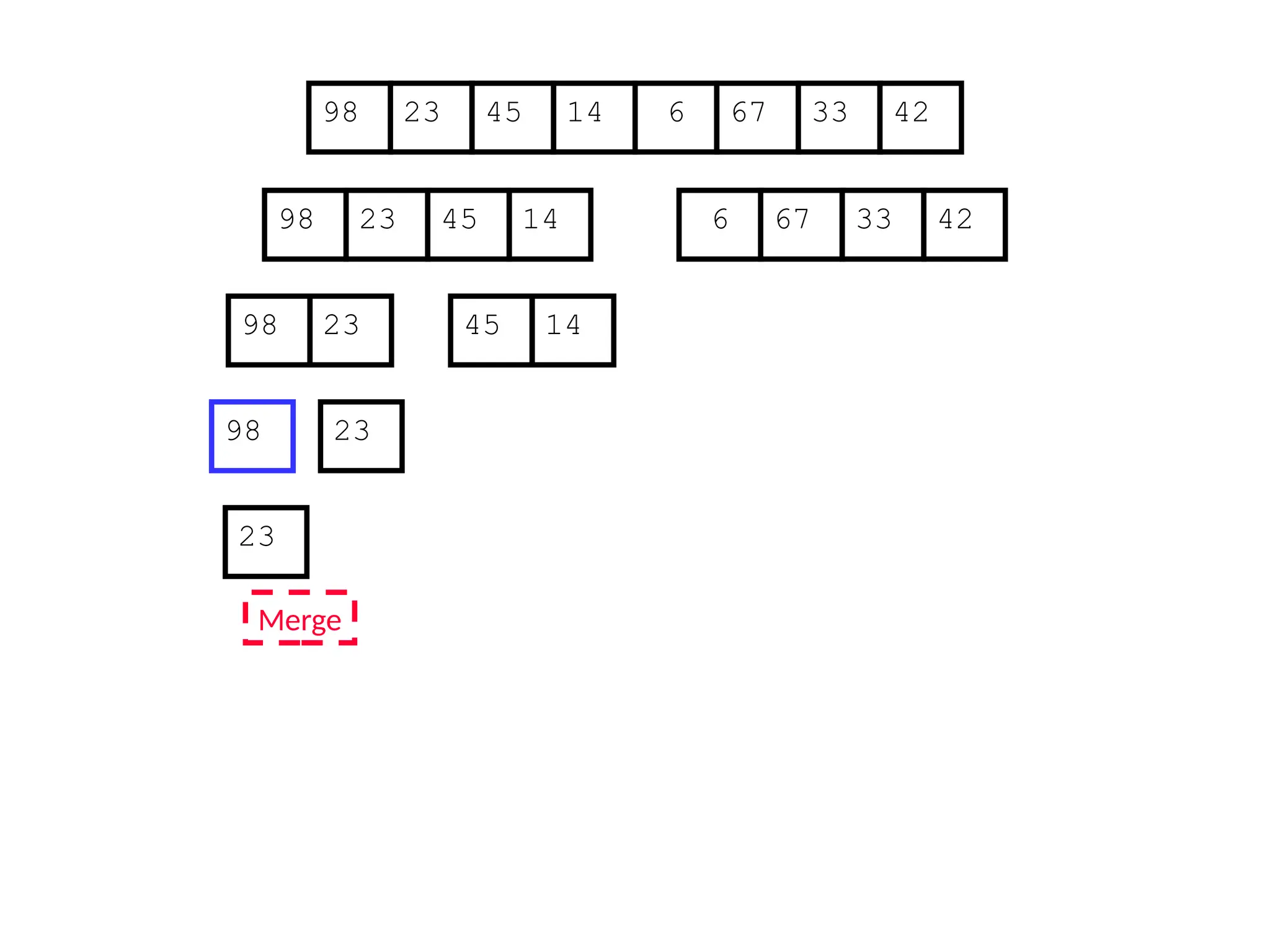
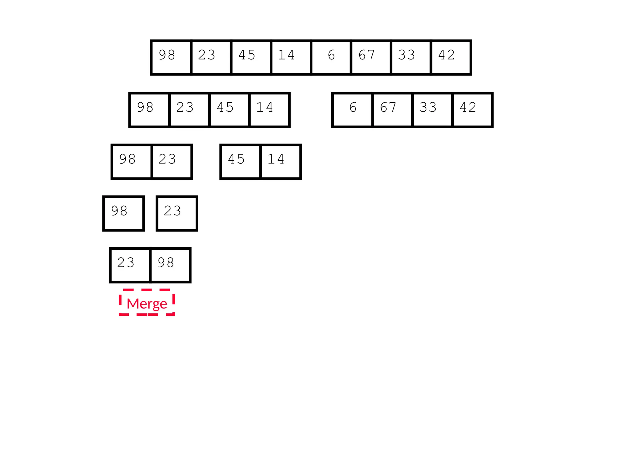
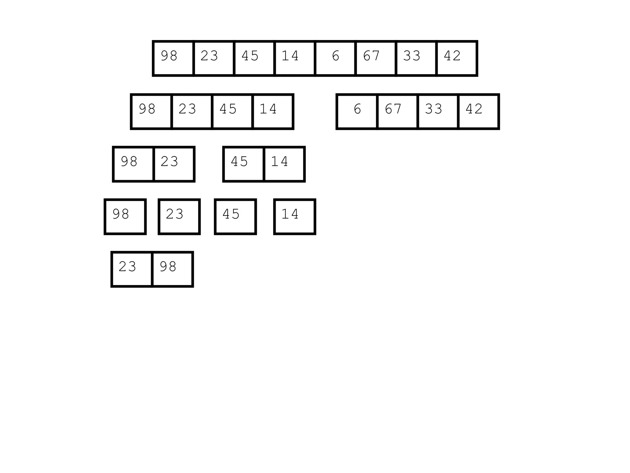
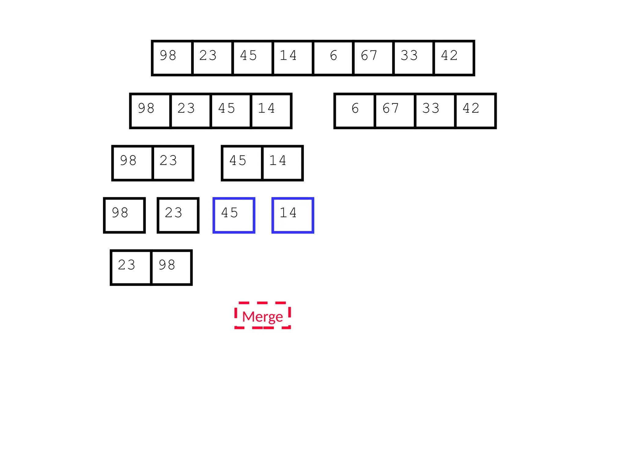
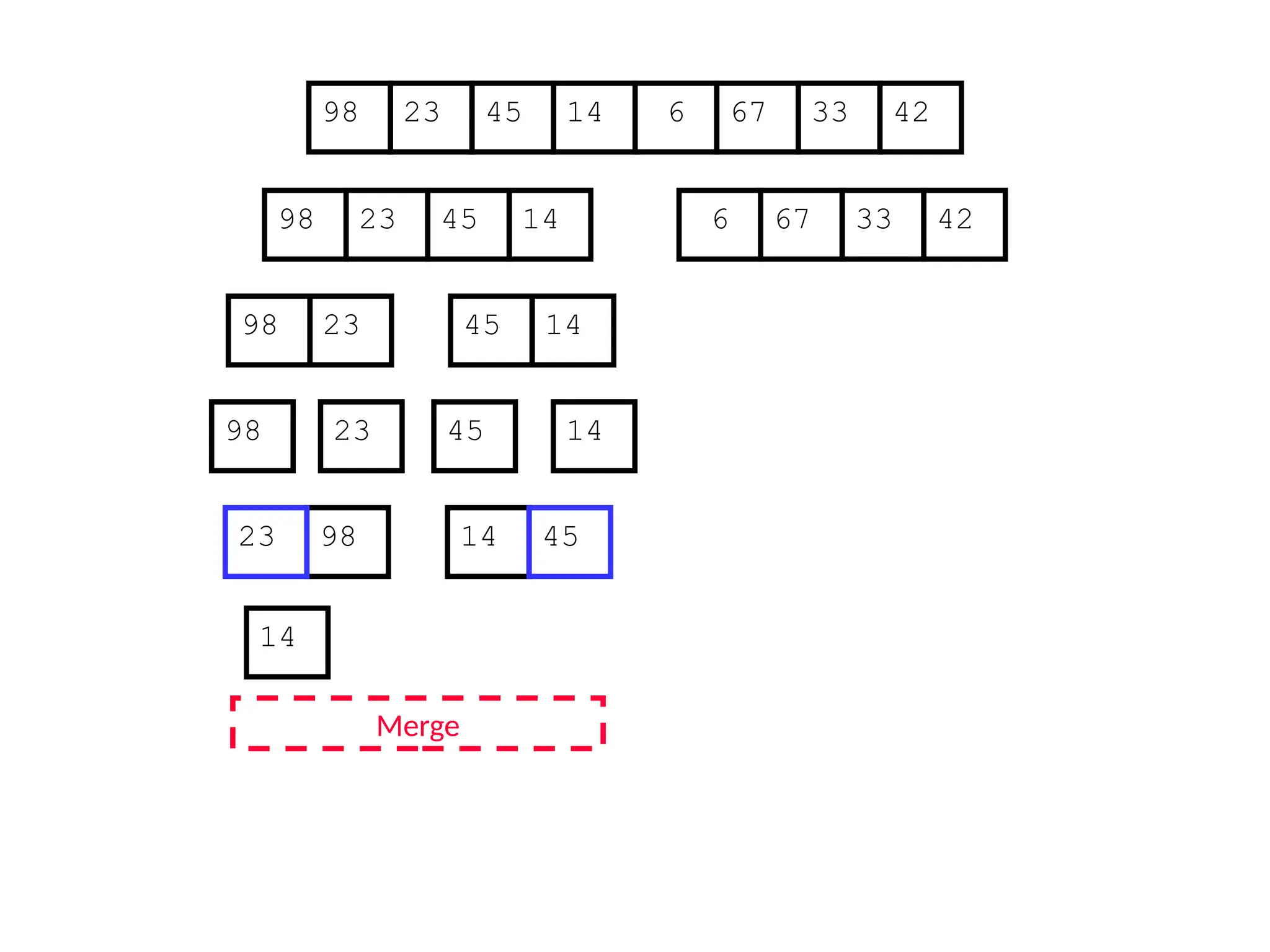
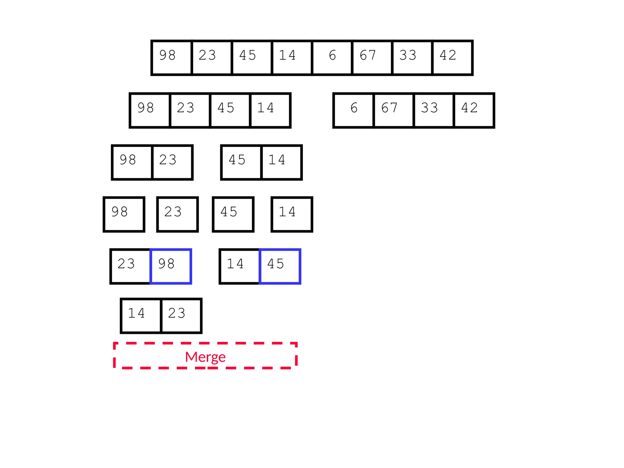
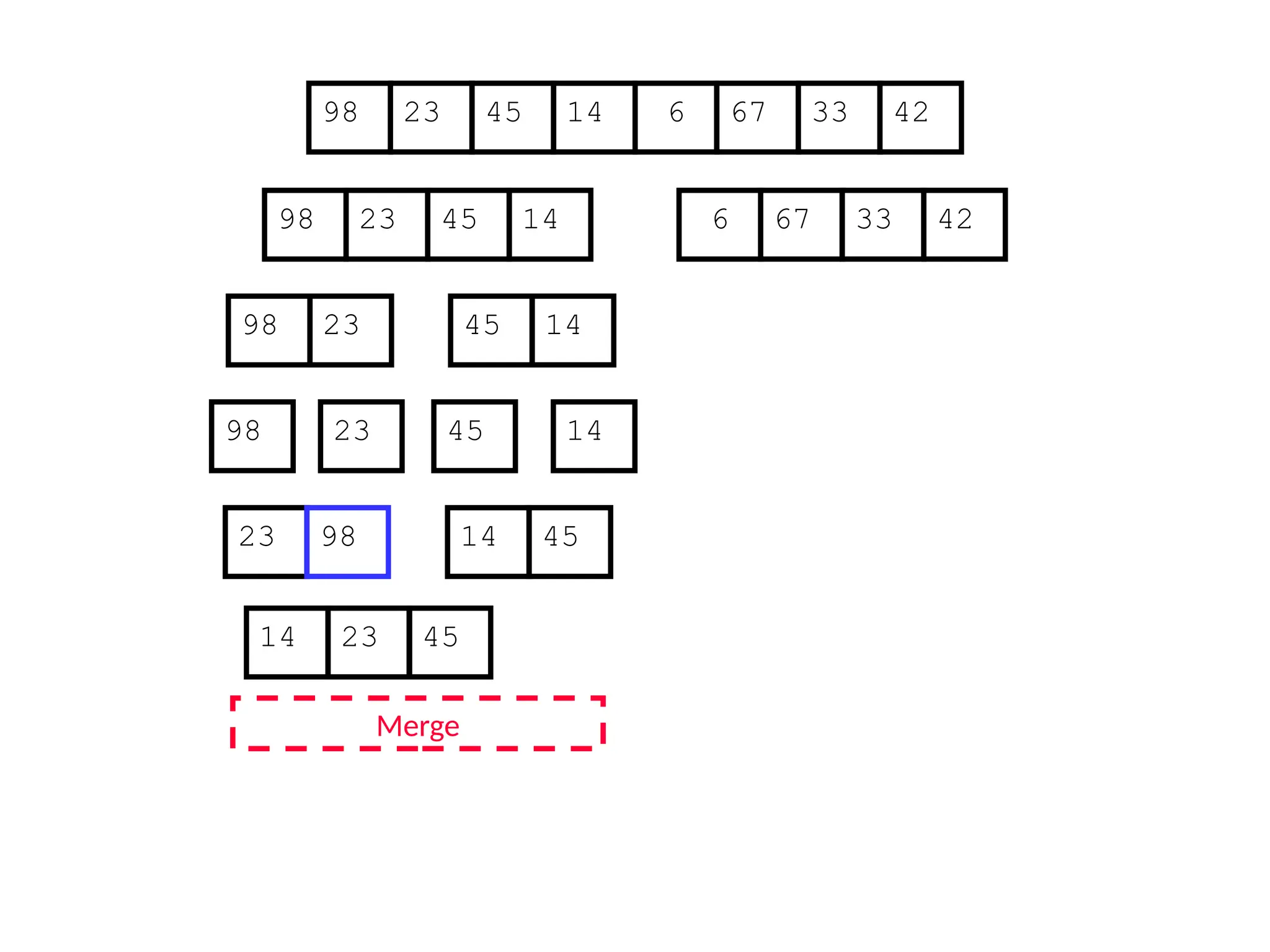
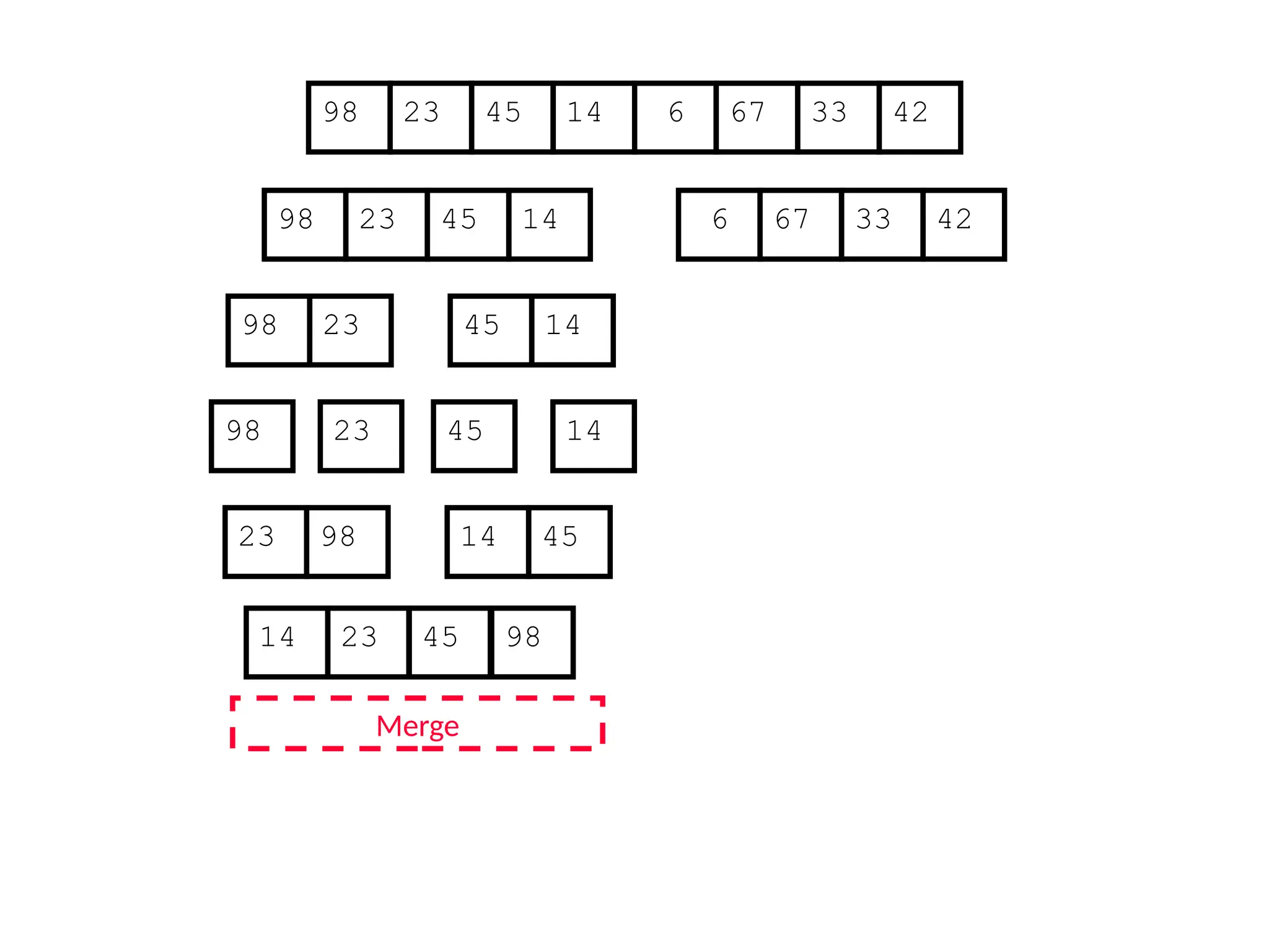
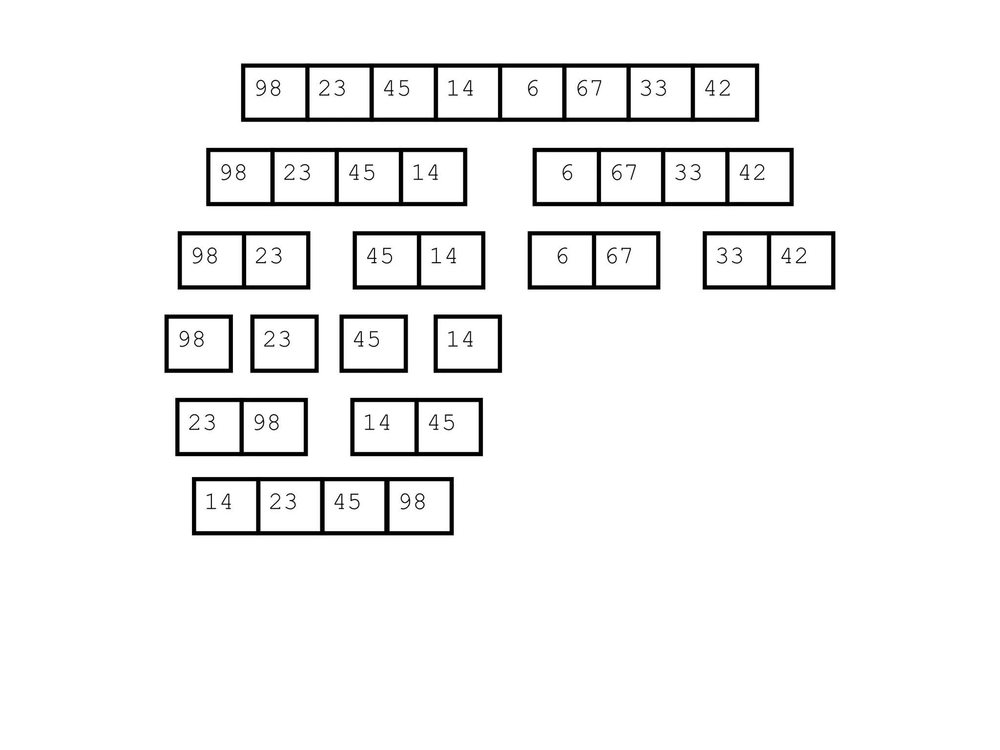
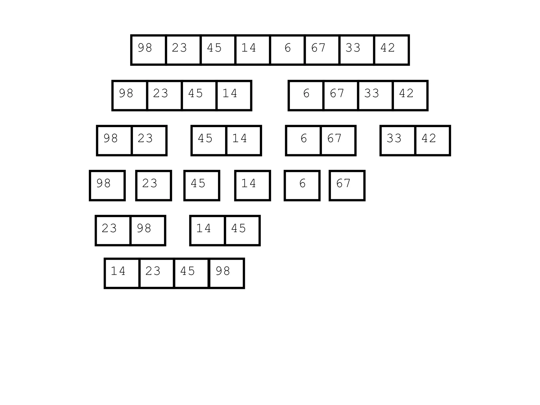
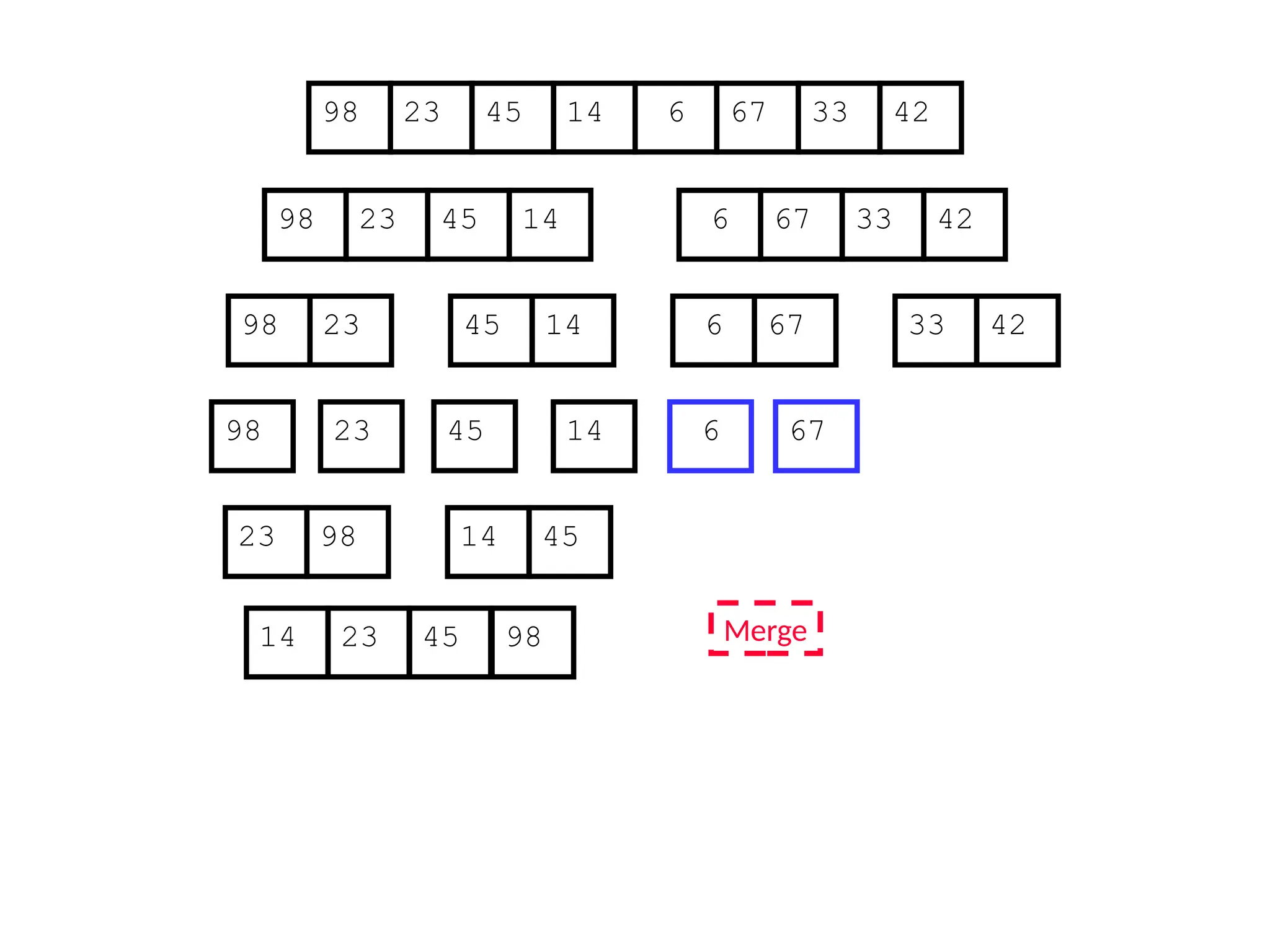
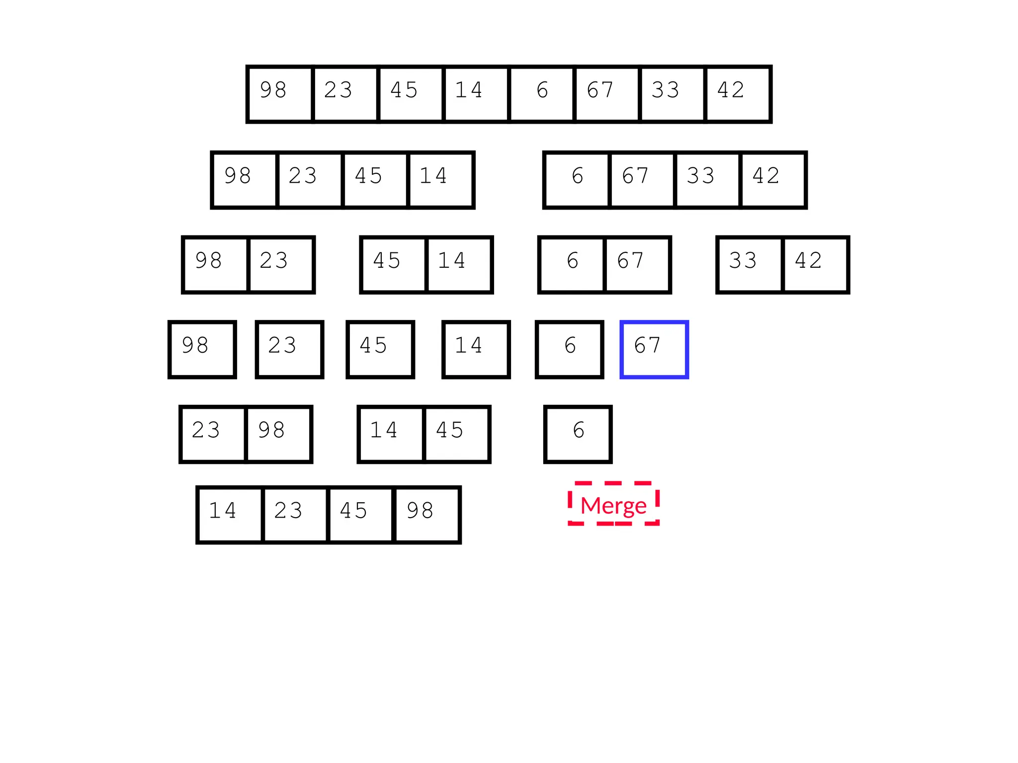
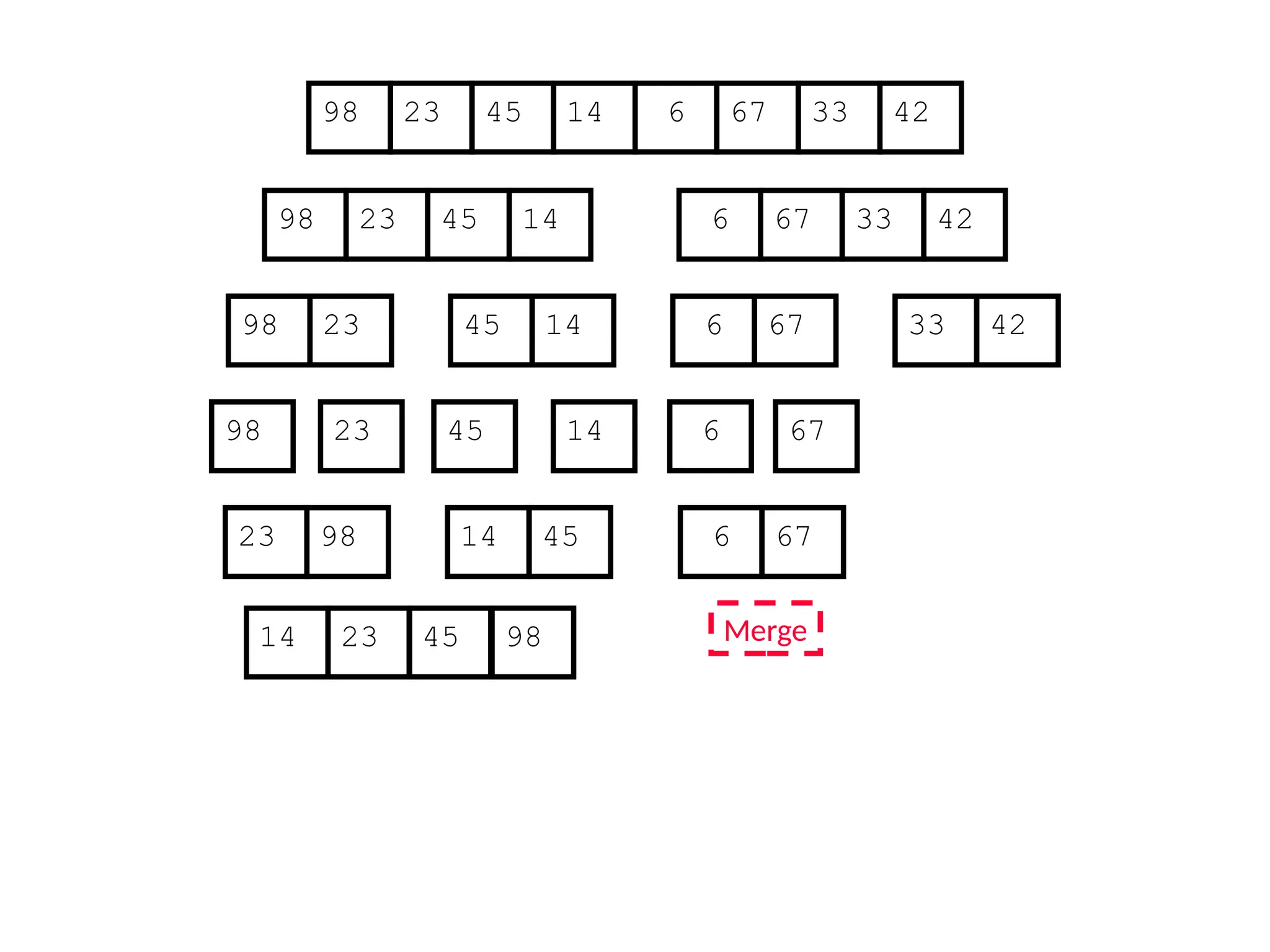
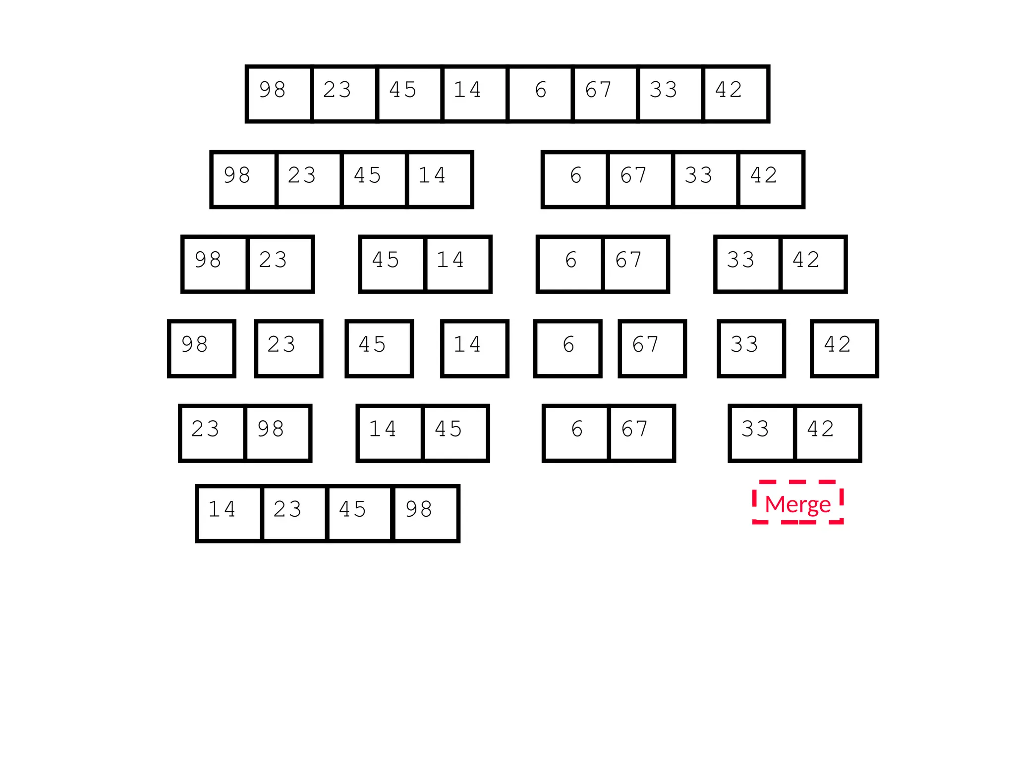
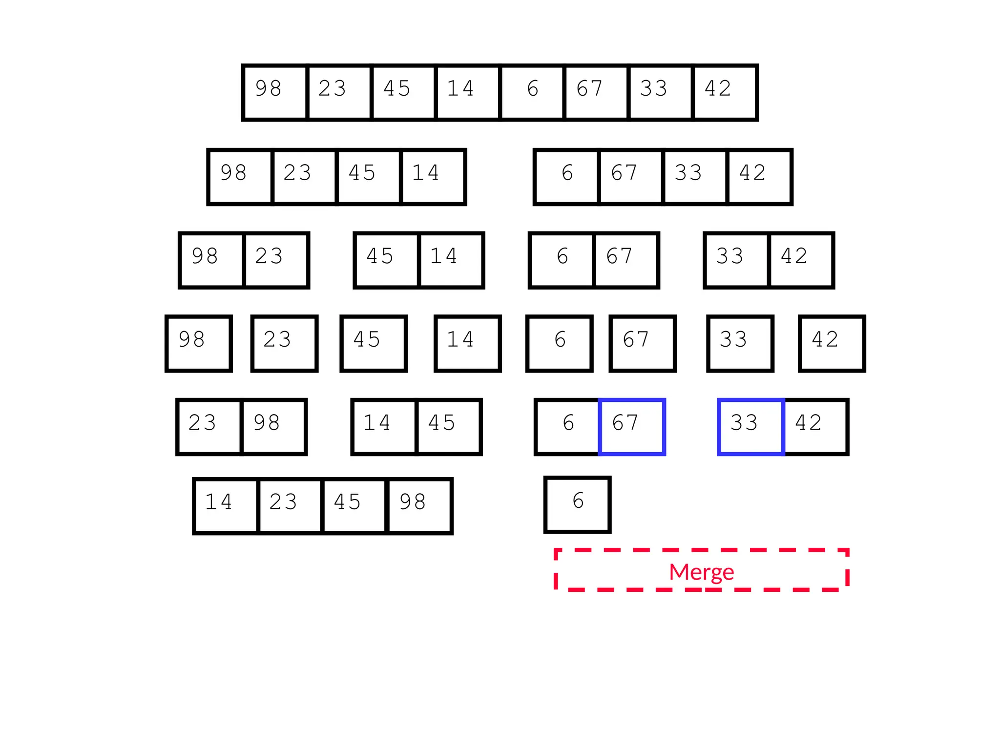
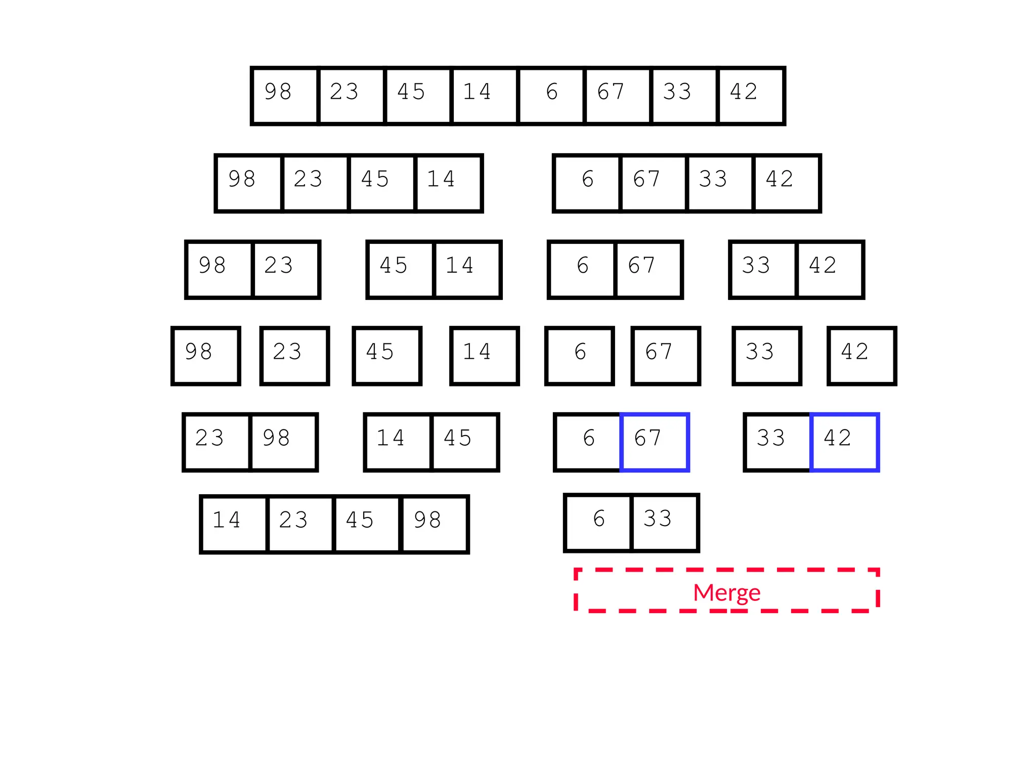
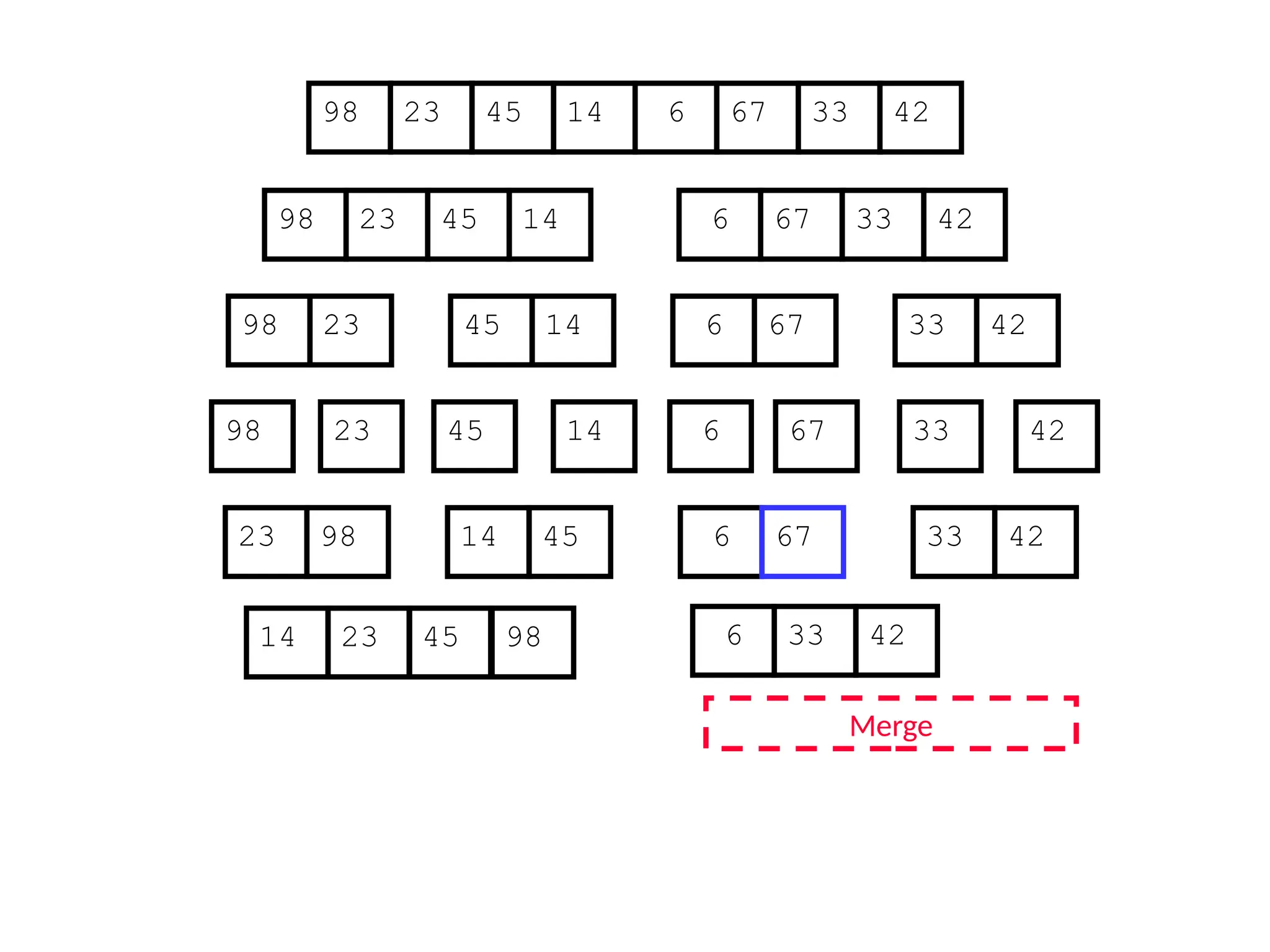
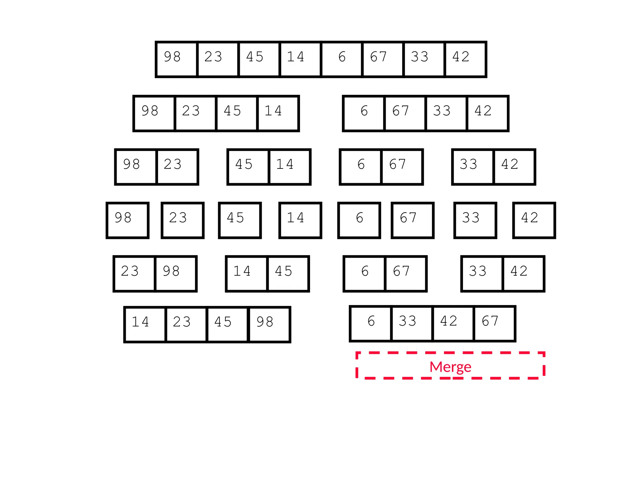
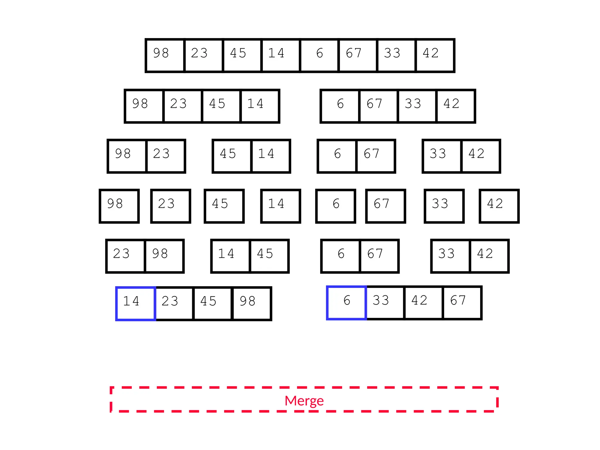
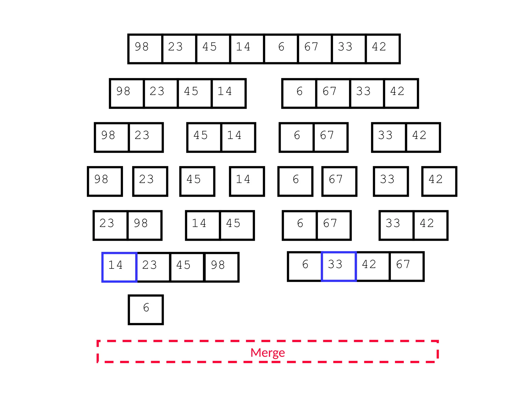
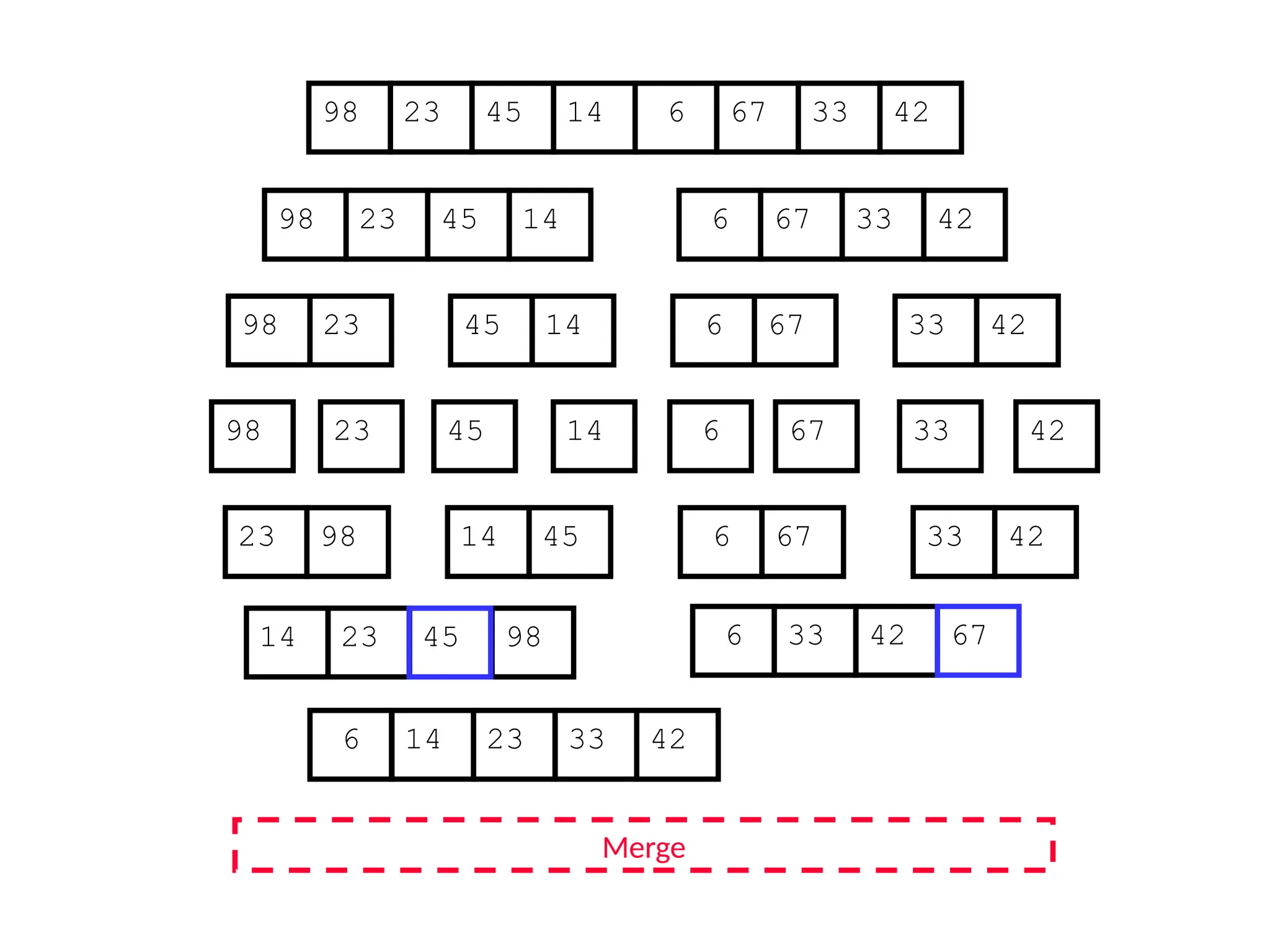
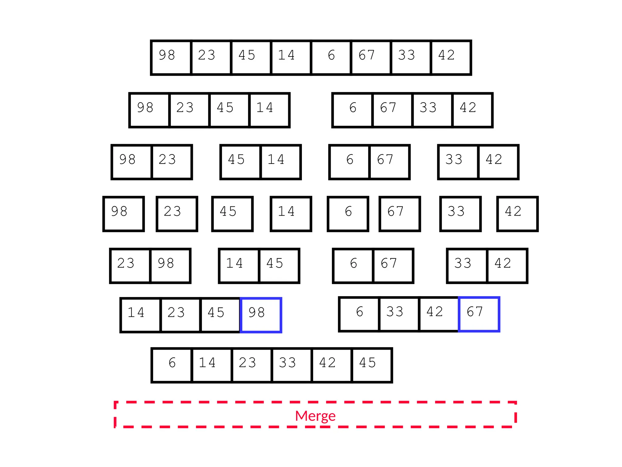
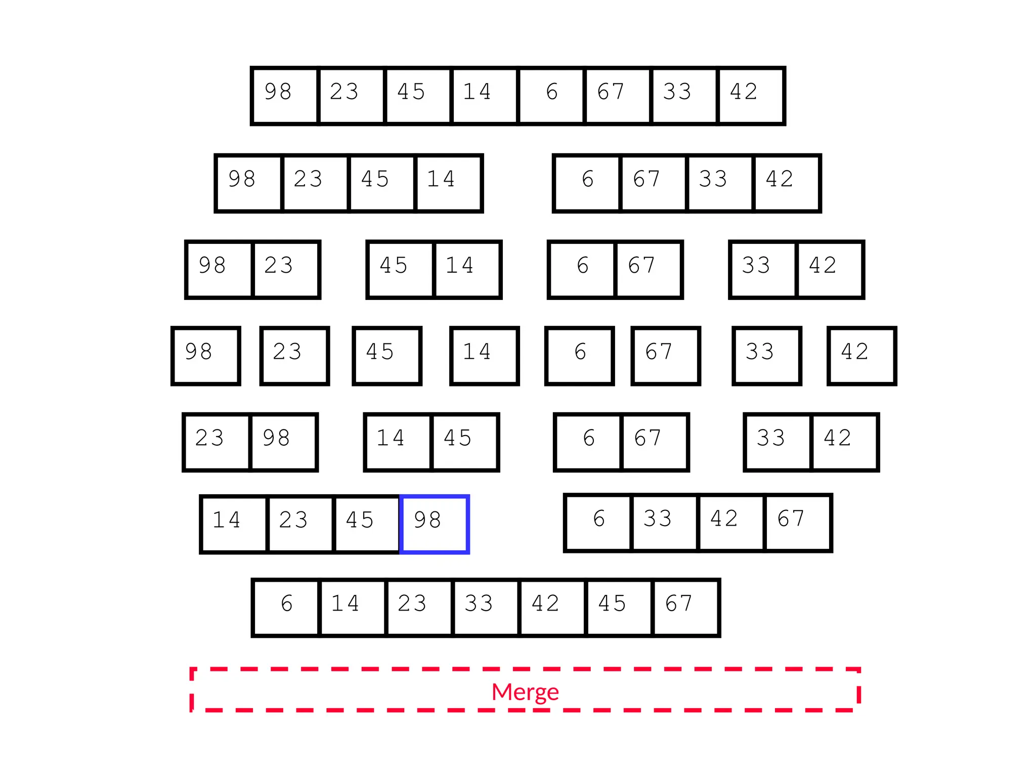
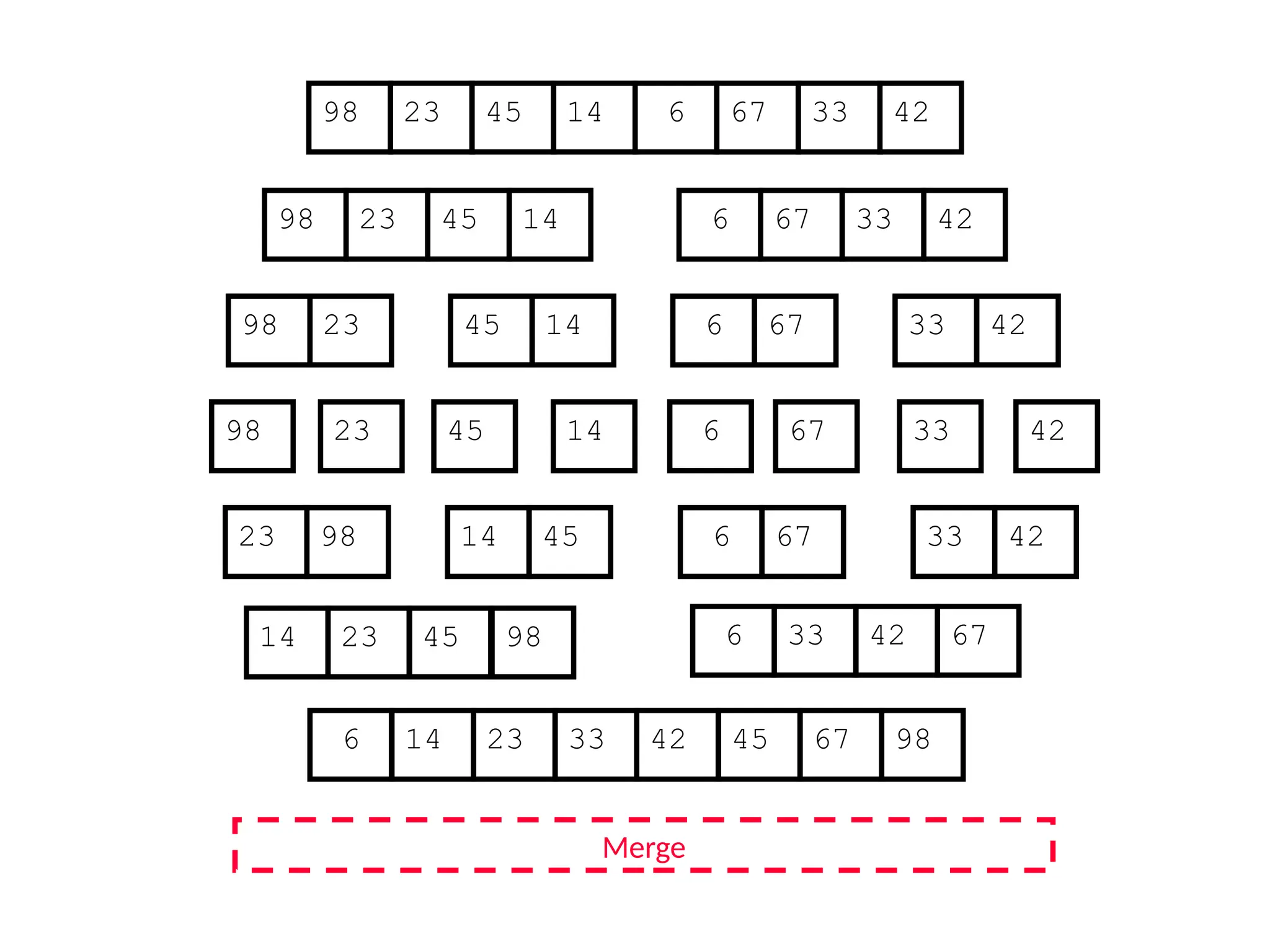
![D&C Example: Merge Sort (Section 2.3)
Sorting Problem: Sort a sequence A of n elements into non-decreasing order:
MergeSort (A[p..r]) //sort A[p..r]
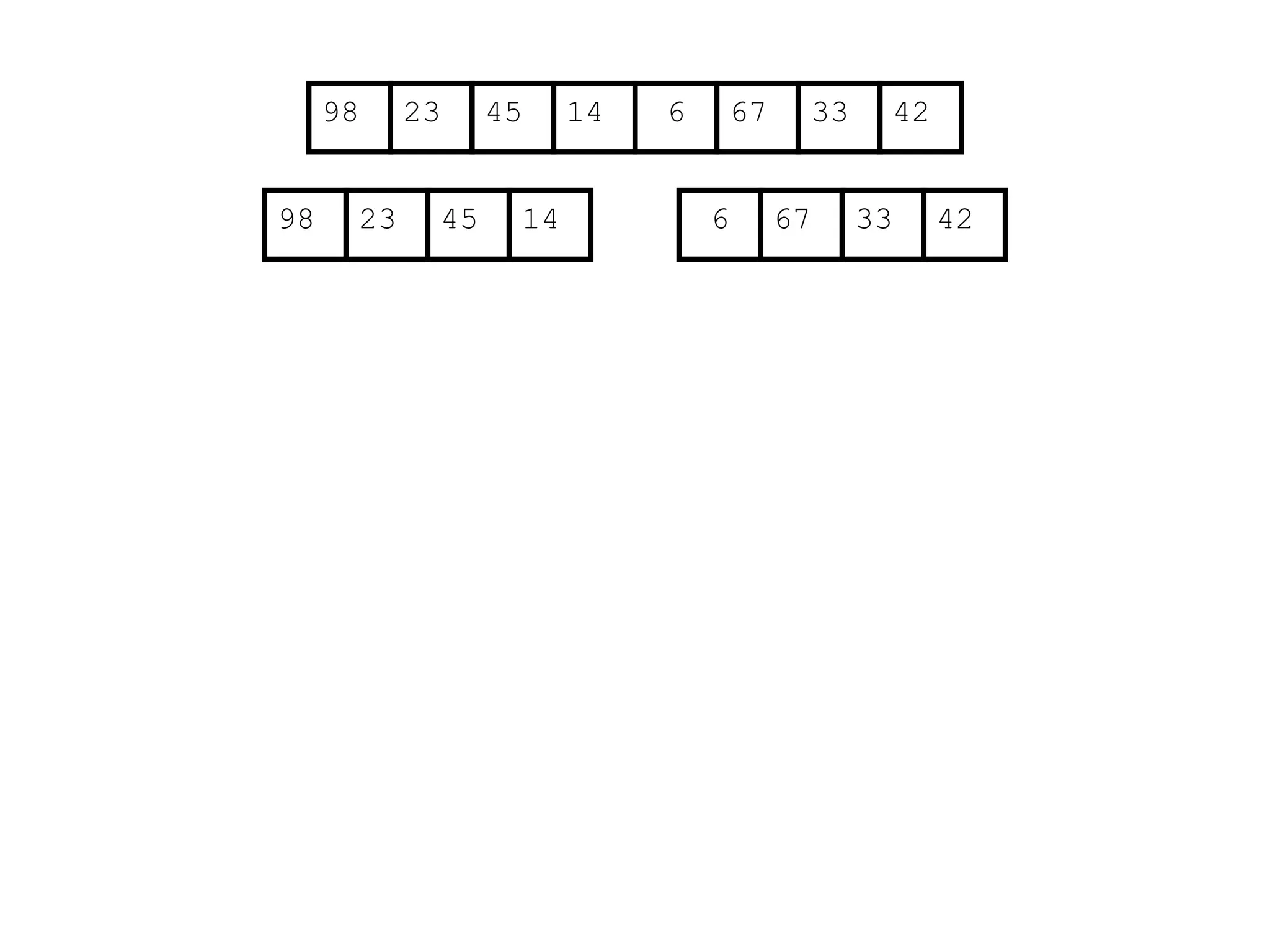
Divide: Divide the n-element input array into two subarray of ≈ n/2 elements
each [easy]:
q (p+r)/2
Conquer: Sort the two subsequences recursively by calling merge sort on
each subsequence [easy]:
MergeSort (A[p .. q]) // A[p .. q] becomes sorted after this call
MergeSort (A[q+1 .. r]) //A[q+1..r] becomes sorted after this call
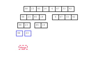
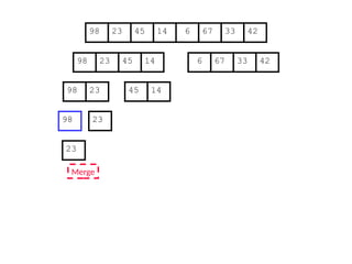
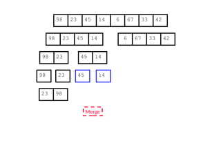
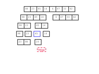
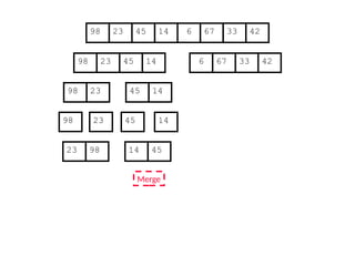
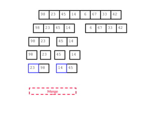
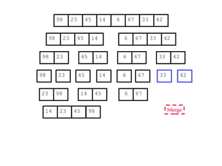
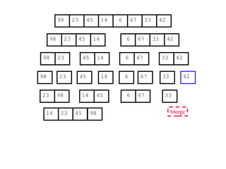
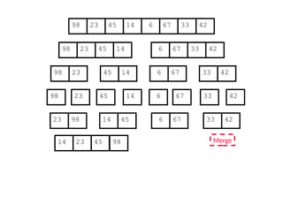
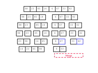
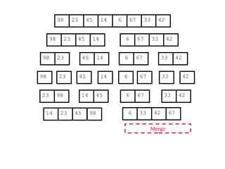
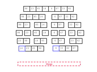
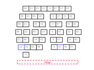
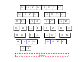
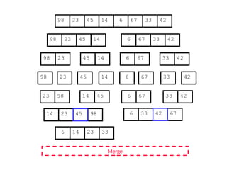
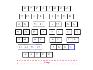
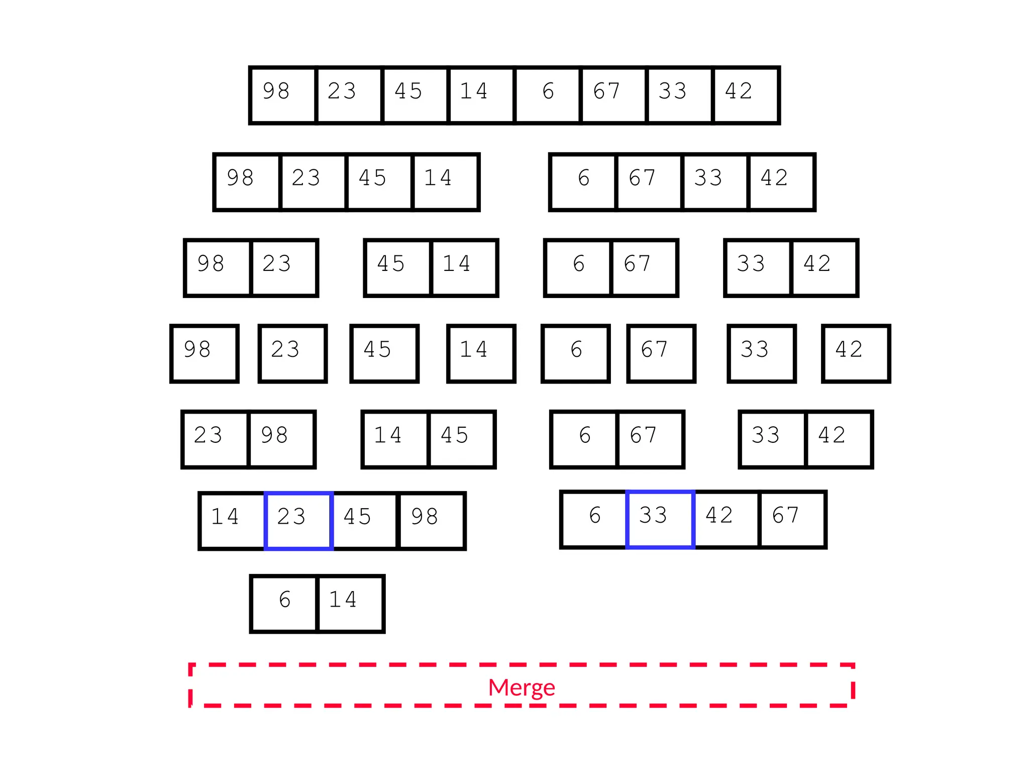
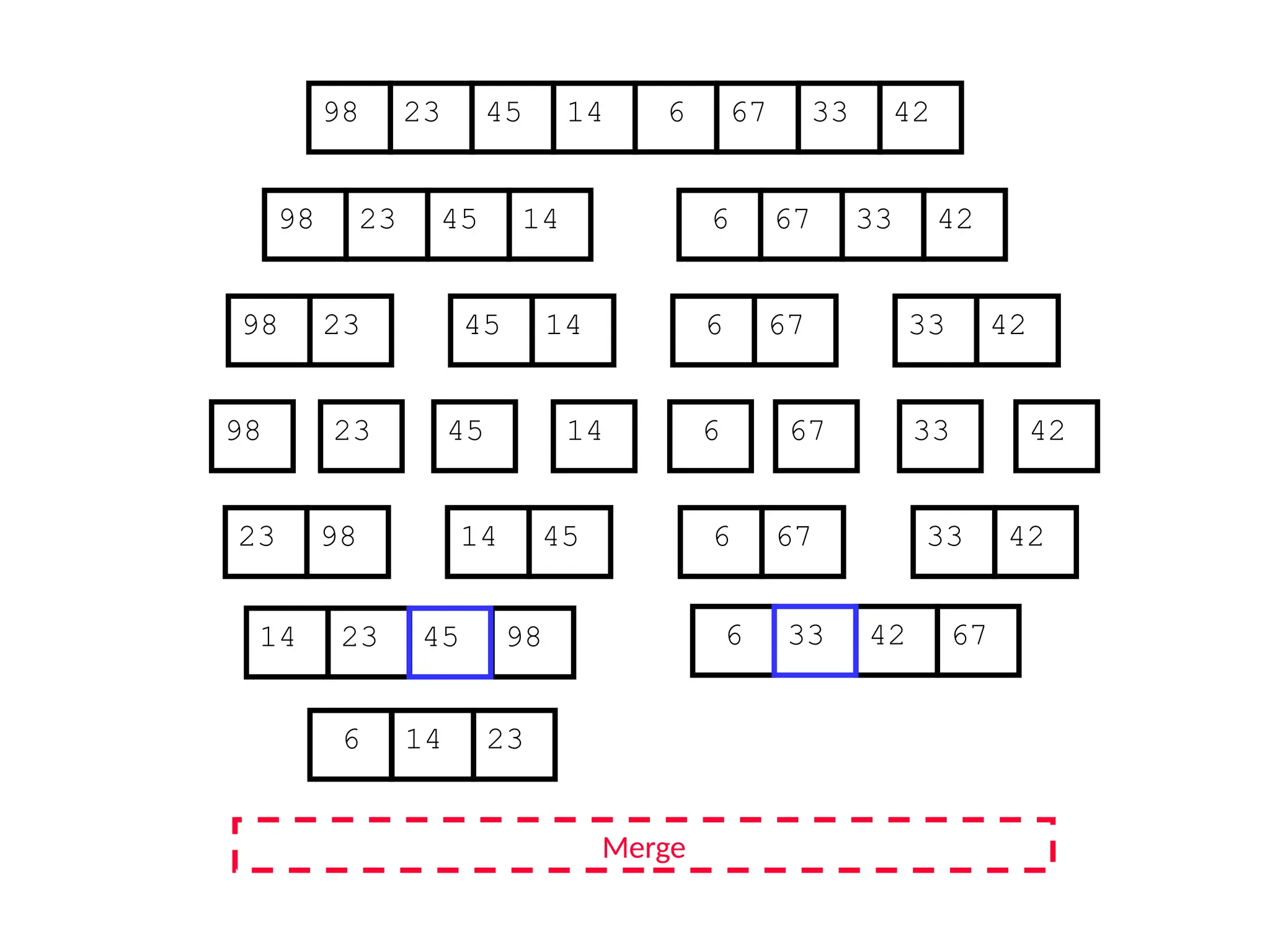
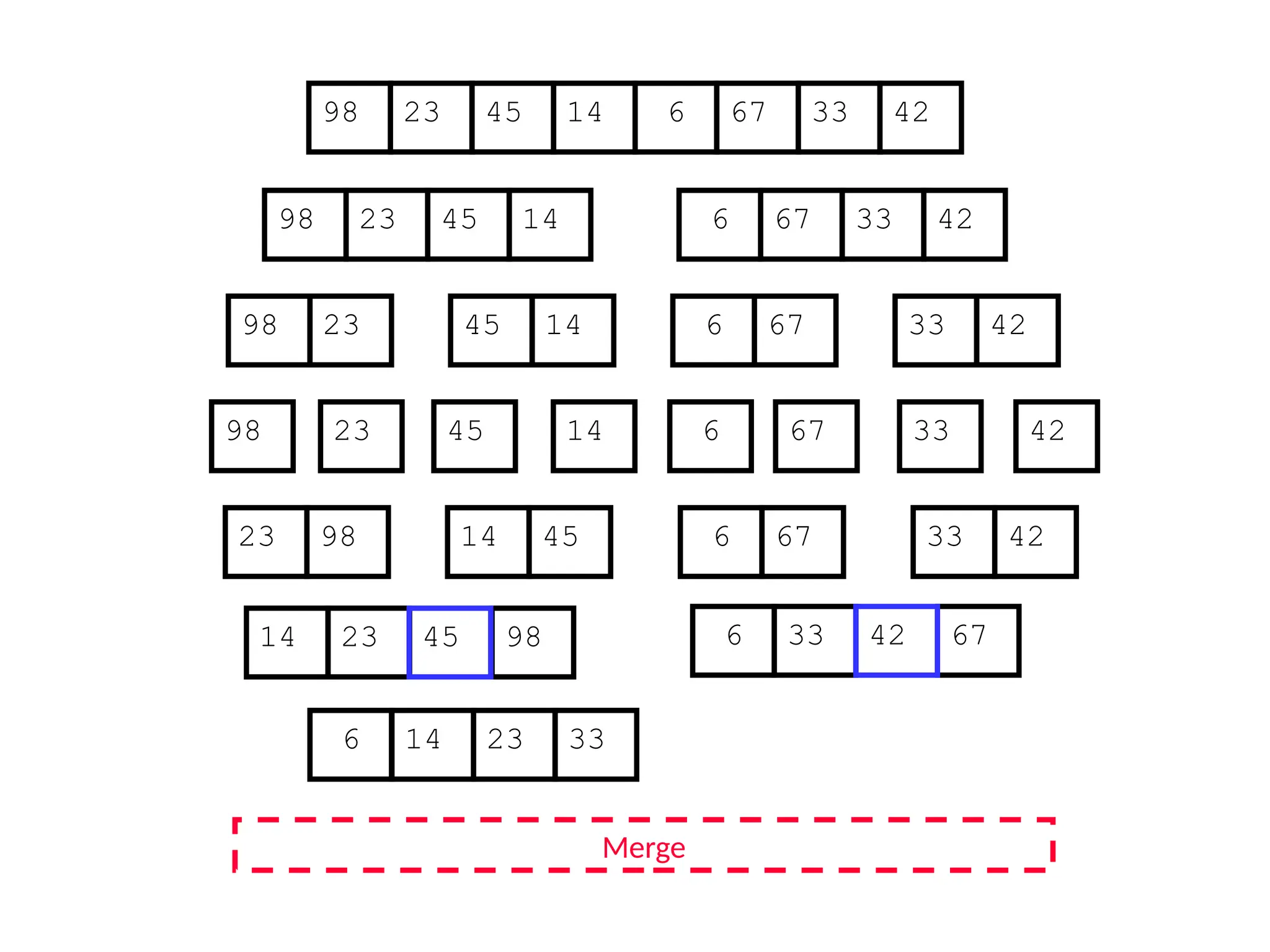
Combine: Merge the two sorted subsequences to produce the sorted
sequence [how?]](https://image.slidesharecdn.com/l2divideconquer-241117011201-6376395f/85/L2_DatabAlgorithm-Basics-with-Design-Analysis-pptx-18-320.jpg)

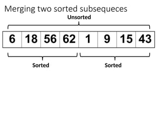
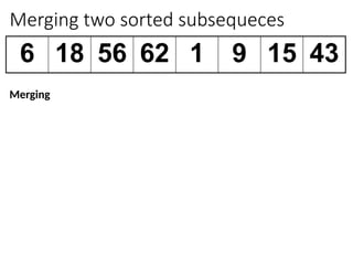
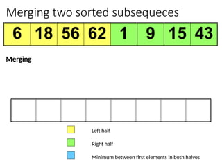
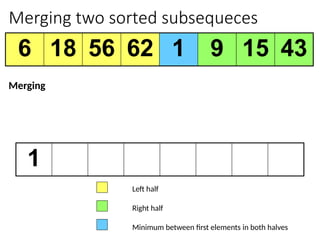
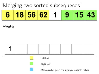
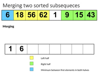
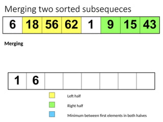
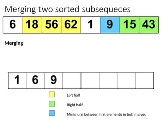
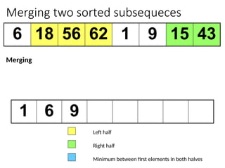
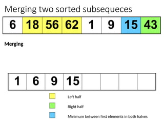
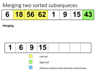
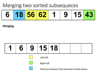
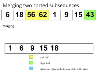
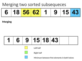
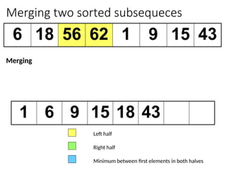
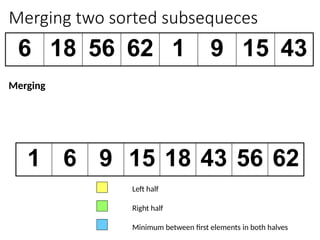
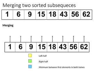
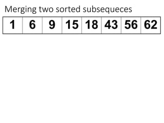
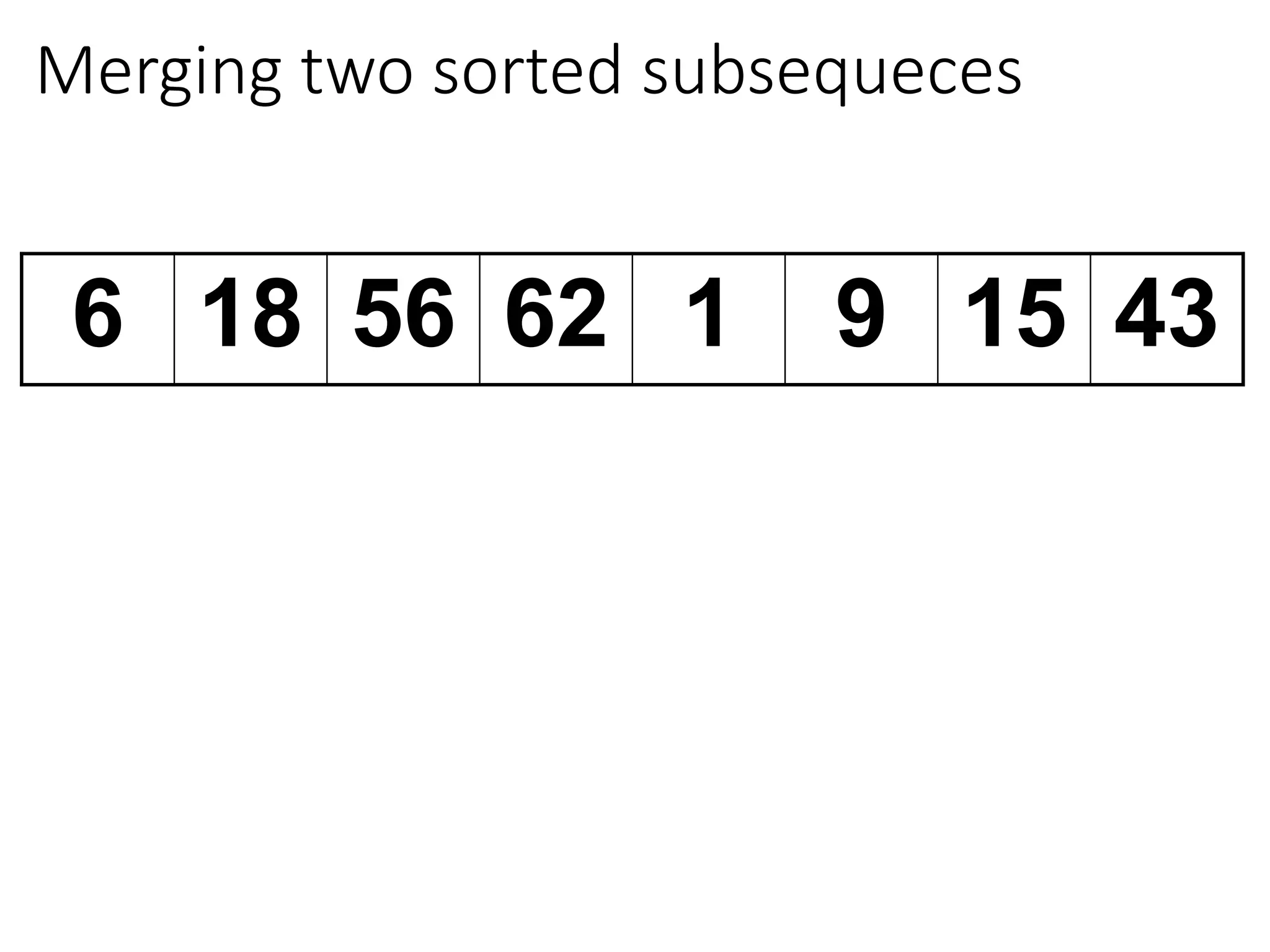
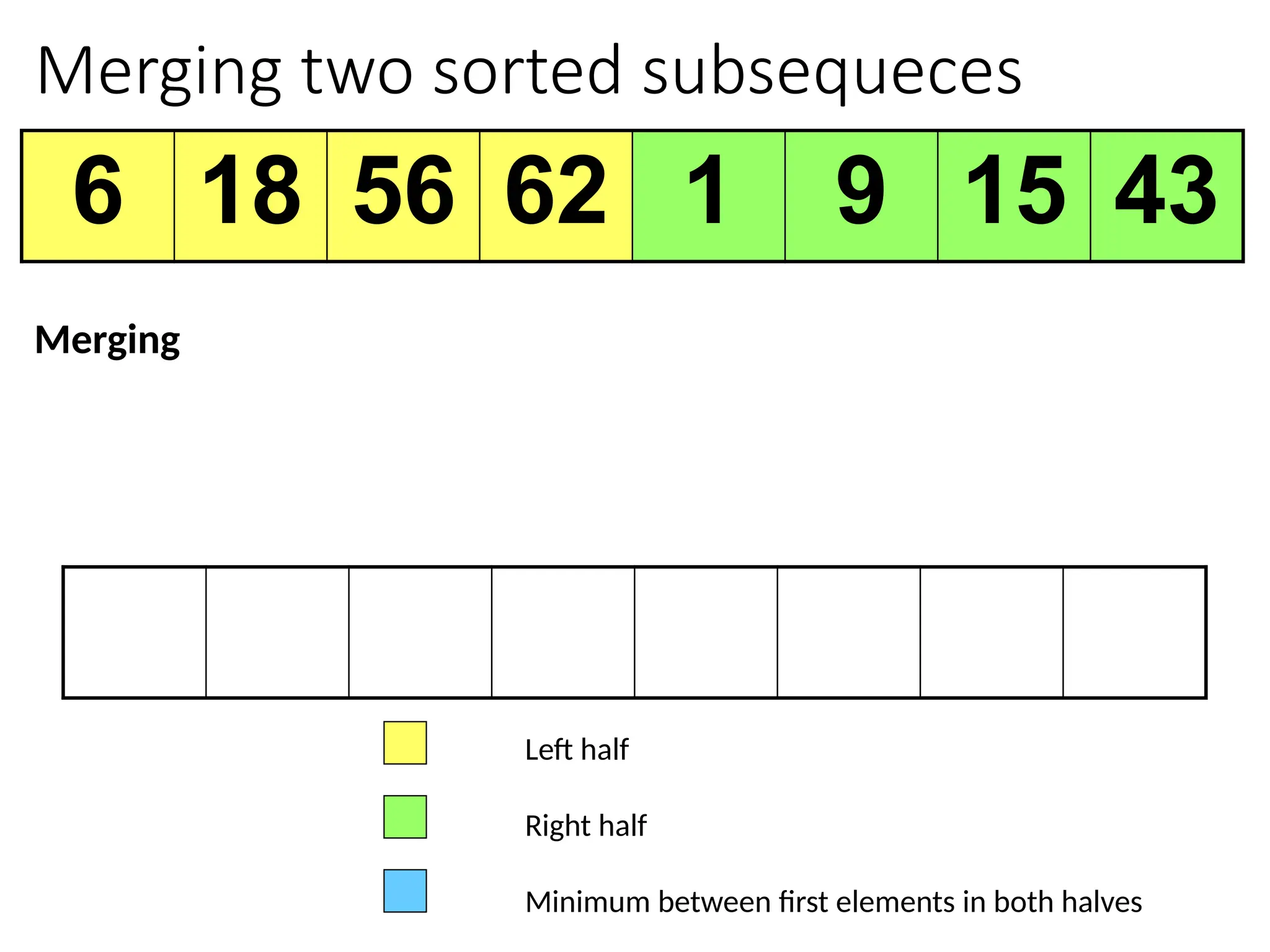
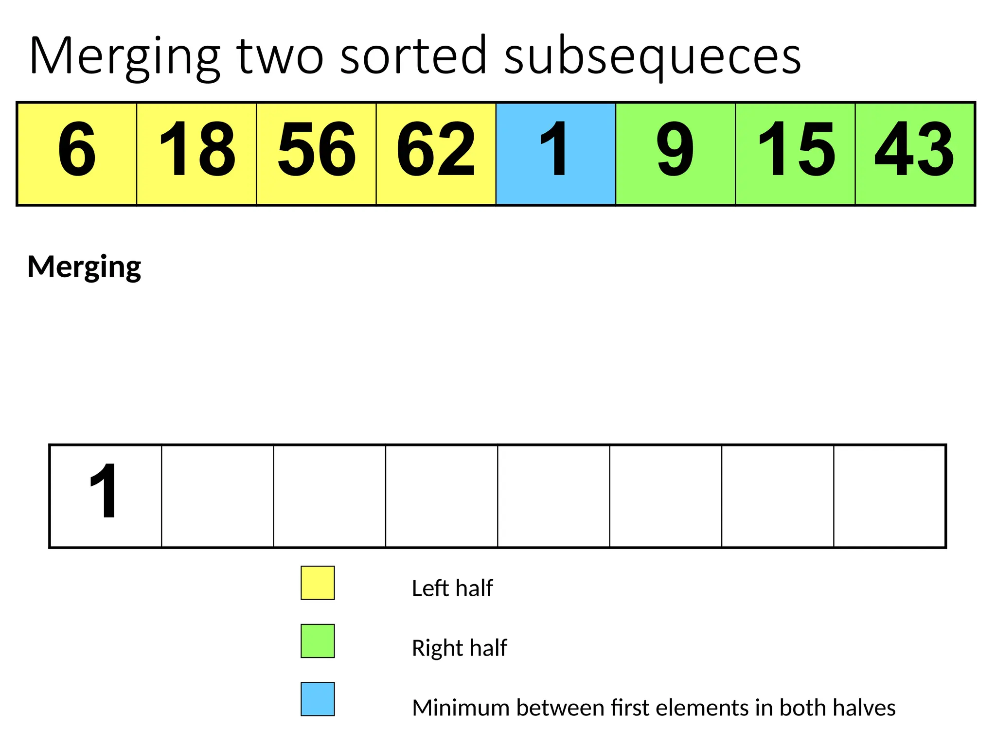
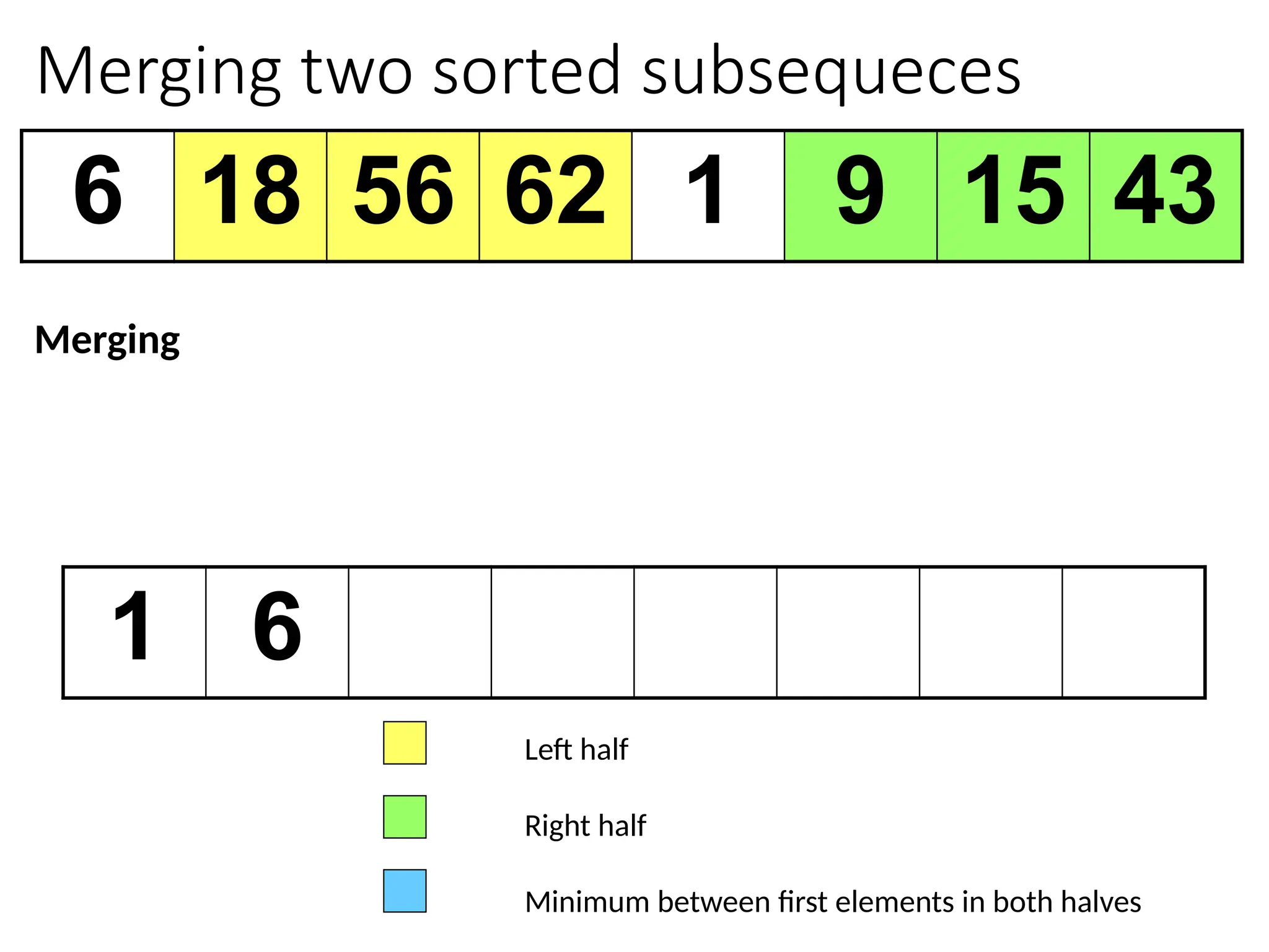
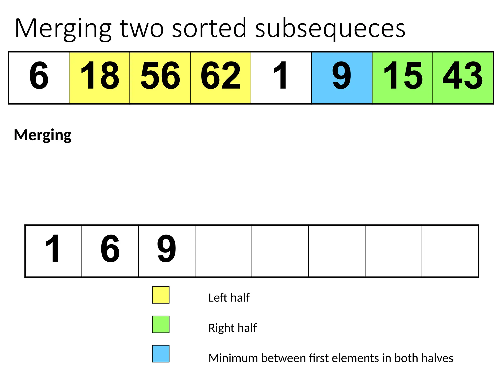
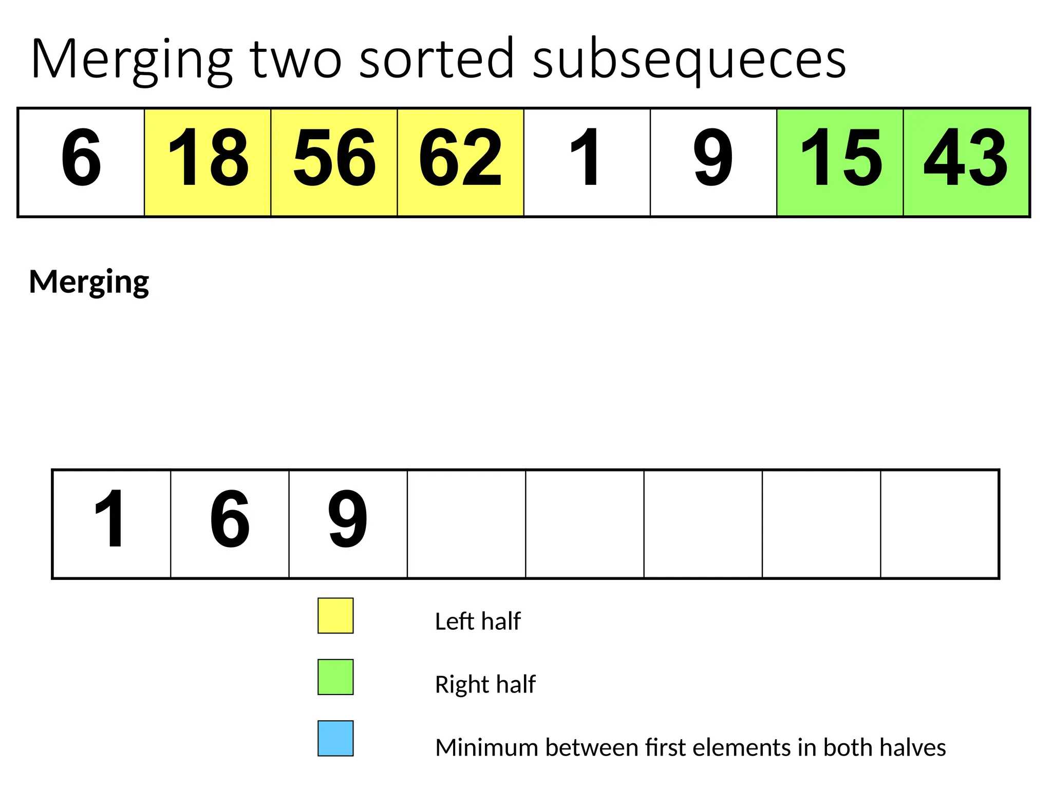
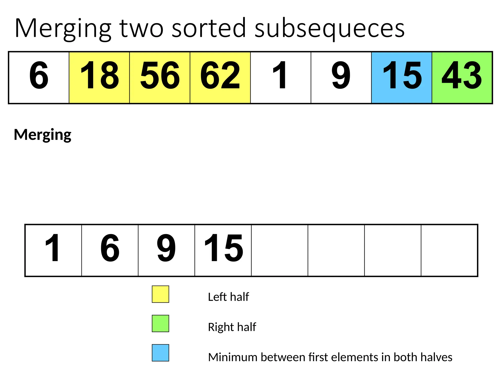
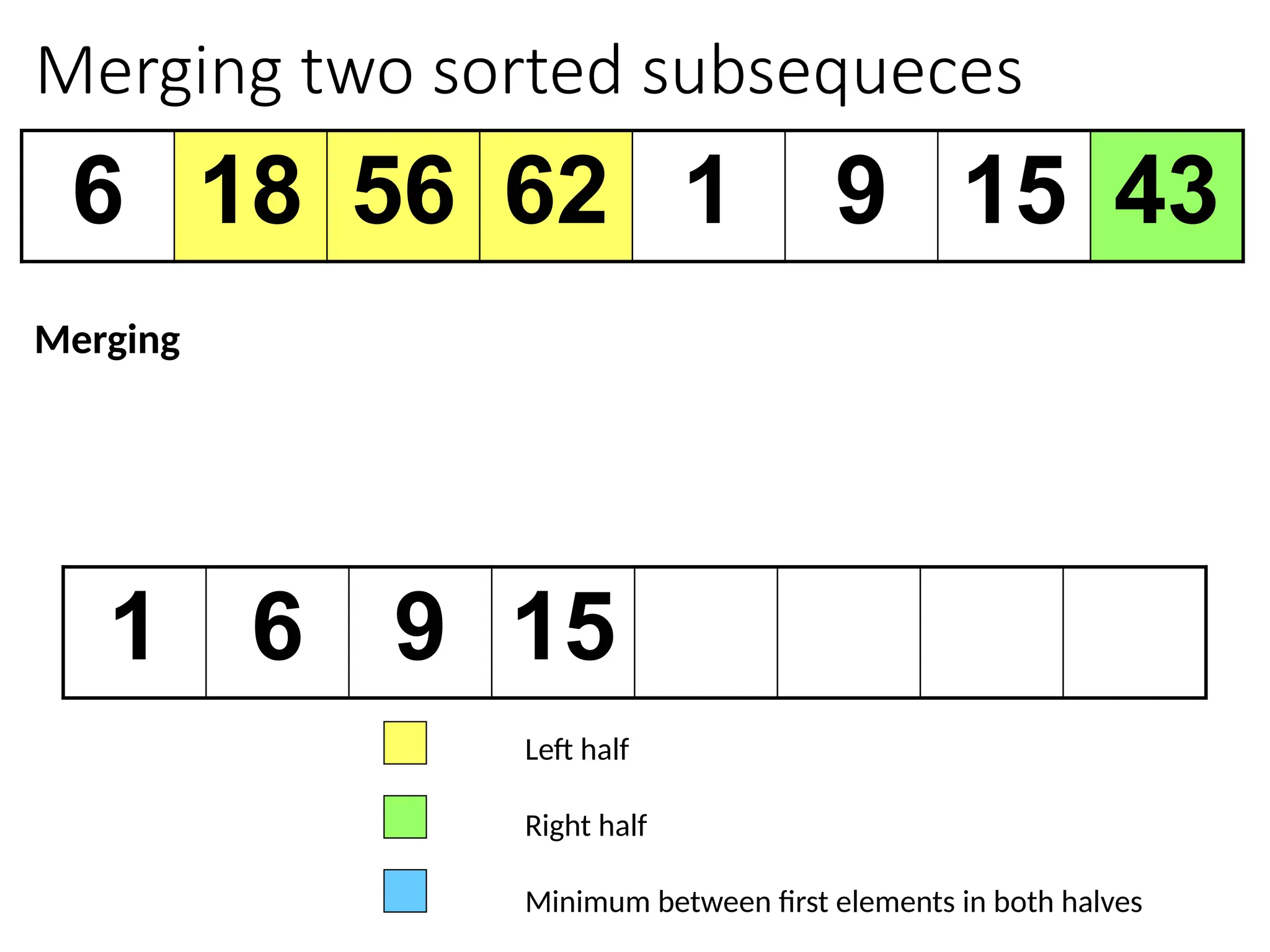
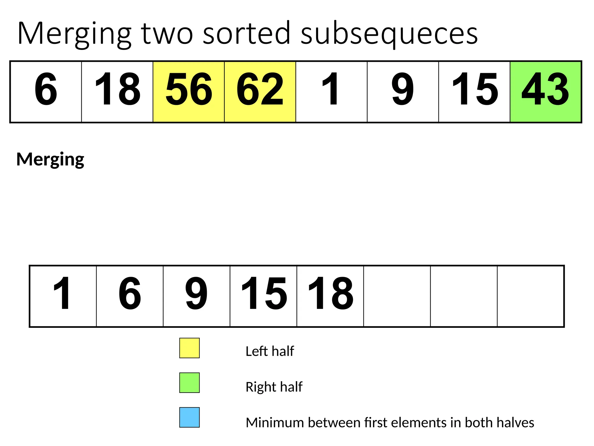
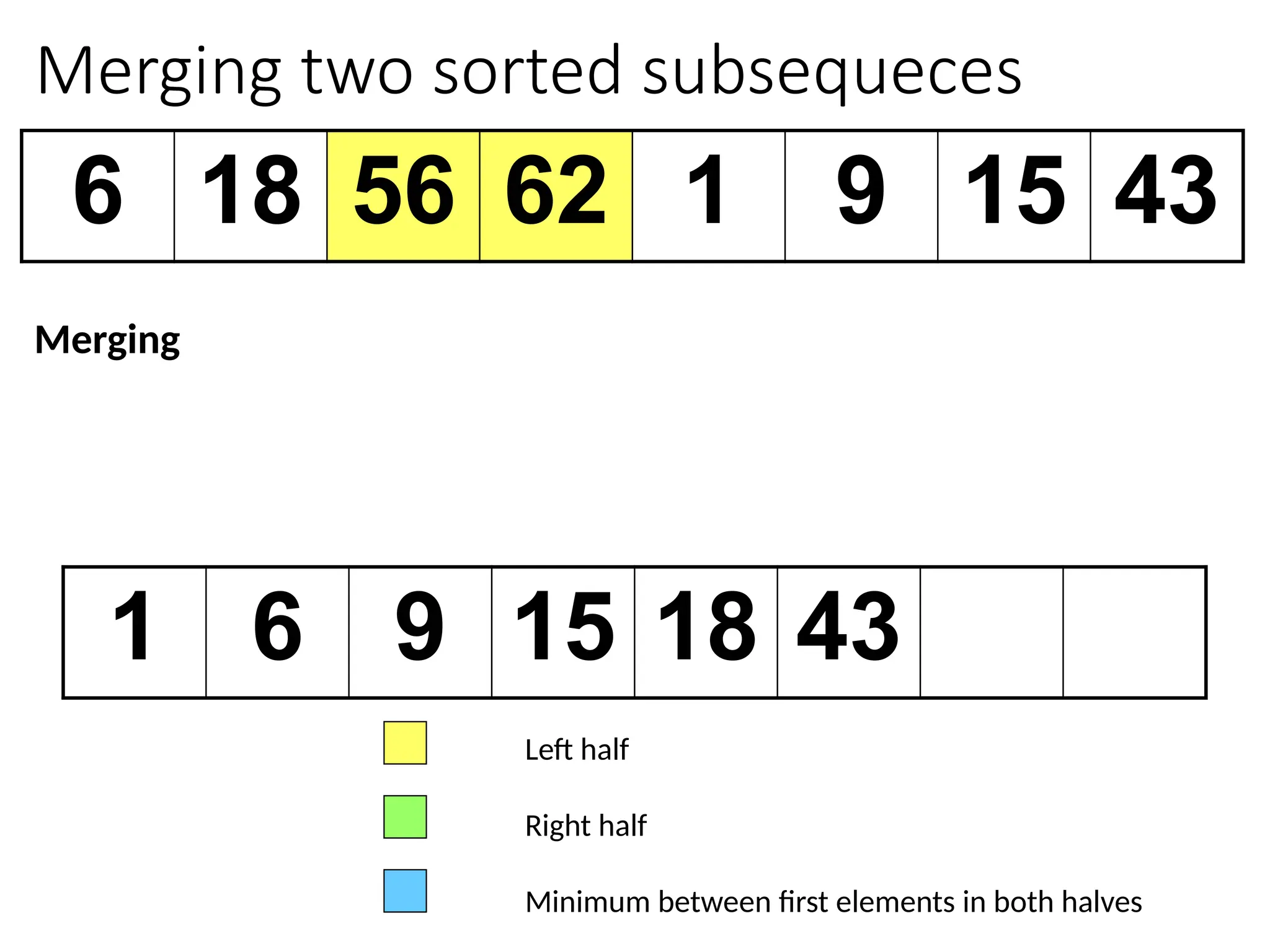
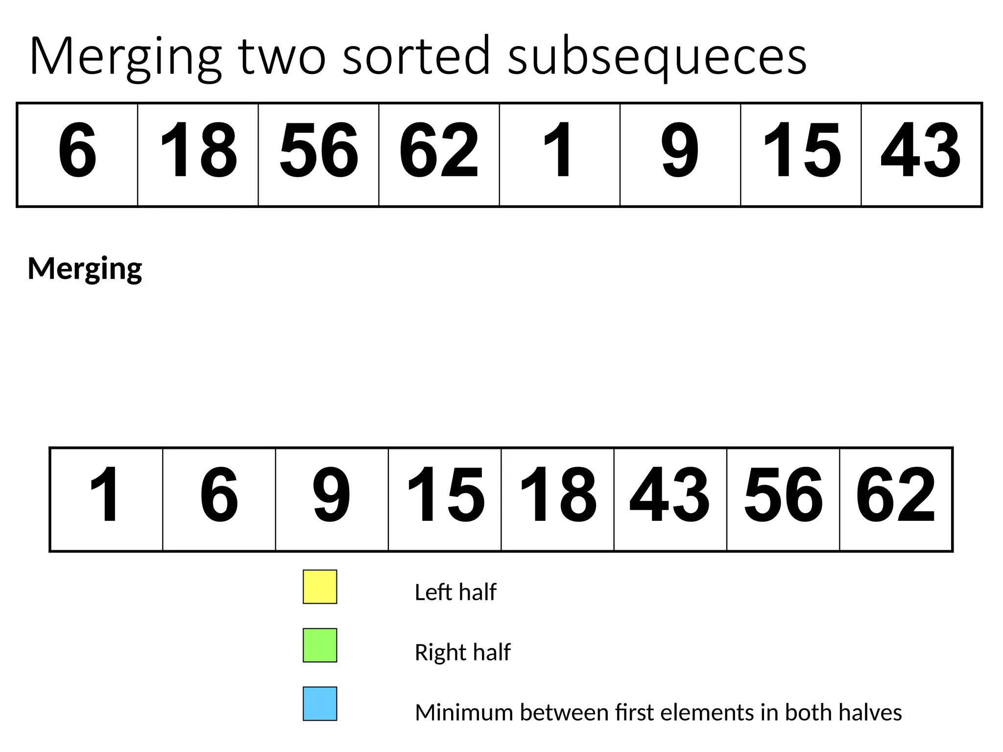
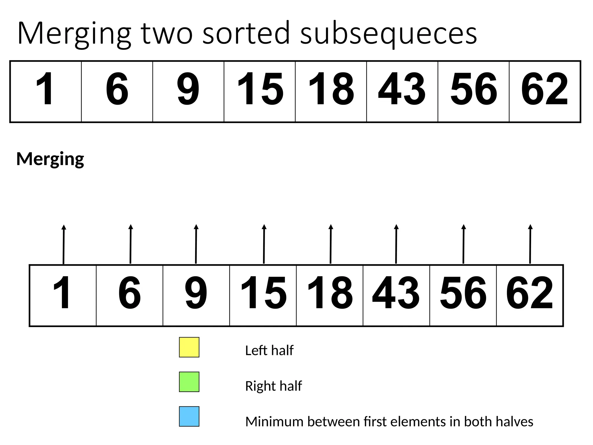
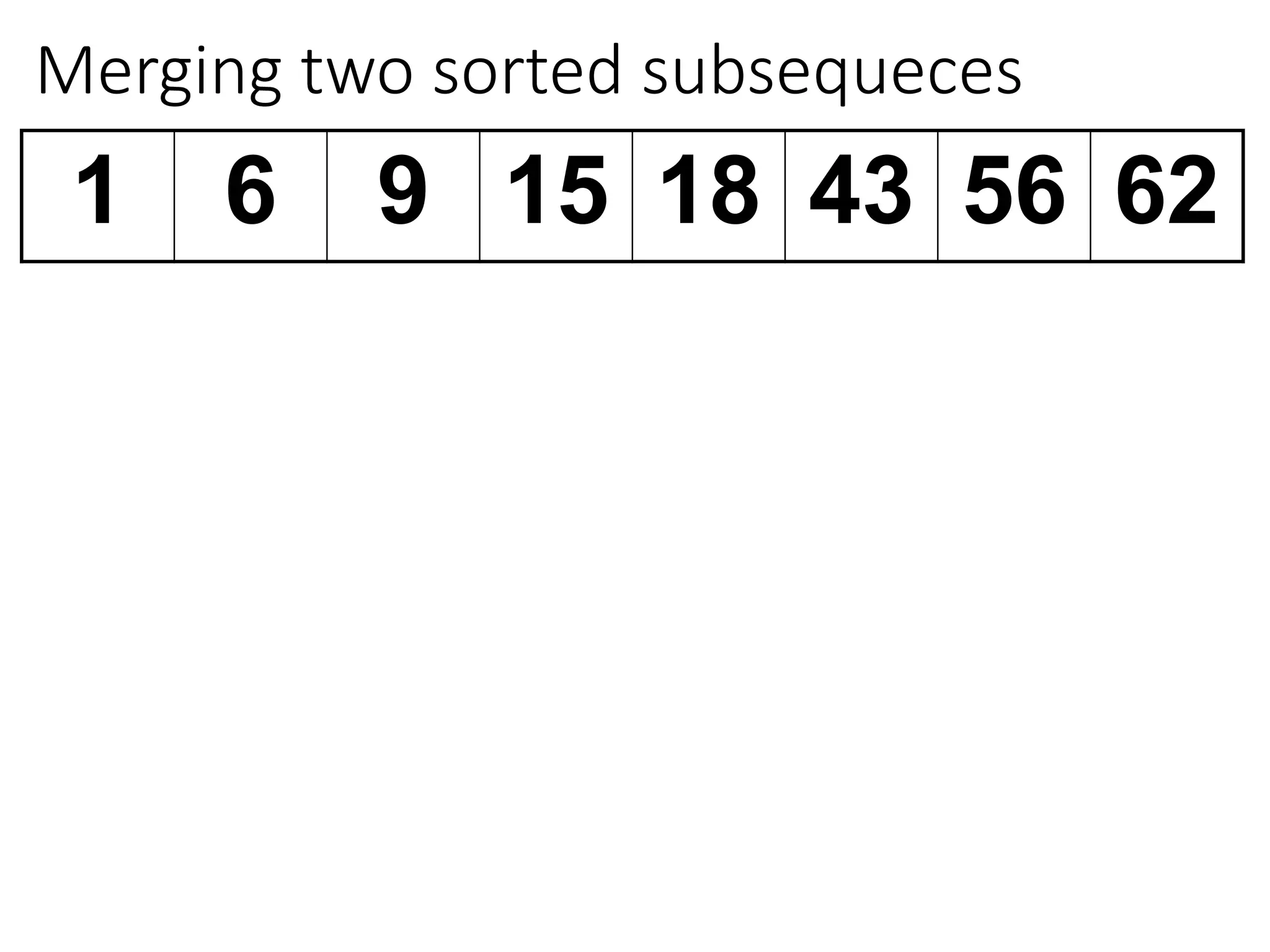
![Merging two sorted subsequeces
Merge(A, p, q, r)
1 n1 q – p + 1
2 n2 r – q
3 for i 1 to n1
4 do L[i] A[p + i – 1]
5 for j 1 to n2
6 do R[j] A[q + j]
7 L[n1+1]
8 R[n2+1]
9 i 1
10 j 1
11 for k p to r
12 do if L[i] R[j]
13 then A[k] L[i]
14 i i + 1
15 else A[k] R[j]
16 j j + 1
Sentinels, to avoid having to
check if either subarray is
fully copied at each step.
Input: Array containing
sorted subarrays A[p..q] and
A[q+1..r].
Output: Merged sorted
subarray in A[p..r].](https://image.slidesharecdn.com/l2divideconquer-241117011201-6376395f/85/L2_DatabAlgorithm-Basics-with-Design-Analysis-pptx-38-320.jpg)
![Time complexity of Merge
Merge(A, p, q, r) //Let r-p+1 = n
1 n1 q – p + 1 //Θ(1)
2 n2 r – q //Θ(1)
3 for i 1 to n1 //Θ(q-p+1)
4 do L[i] A[p + i – 1]
5 for j 1 to n2 //Θ(r-q)
6 do R[j] A[q + j]
7 L[n1+1]
8 R[n2+1]
9 i 1
10 j 1
11 for k p to r //Θ(r-p+1) = Θ(n)
12 do if L[i] R[j]
13 then A[k] L[i]
14 i i + 1
15 else A[k] R[j]
16 j j + 1
//Total time: Θ(n)
Input: Array containing
sorted subarrays A[p..q] and
A[q+1..r].
Output: Merged sorted
subarray in A[p..r].](https://image.slidesharecdn.com/l2divideconquer-241117011201-6376395f/85/L2_DatabAlgorithm-Basics-with-Design-Analysis-pptx-39-320.jpg)
![Merge Sort (recursive/D&C version)
MergeSort (A, p, r) // sort A[p..r] via merge sort
1 if p < r
2 then q (p+r)/2 //divide
3 MergeSort (A, p, q) //conquer
4 MergeSort (A, q+1, r) //conquer
5 Merge (A, p, q, r) //combine: merge A[p..q] with A[q+1..r]
Initial Call: MergeSort(A, 1, n)](https://image.slidesharecdn.com/l2divideconquer-241117011201-6376395f/85/L2_DatabAlgorithm-Basics-with-Design-Analysis-pptx-40-320.jpg)


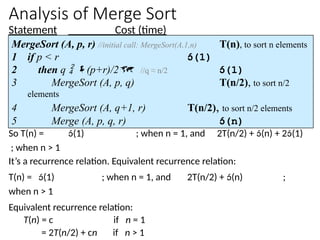
![Analysis of Merge Sort
Statement Cost
MergeSort (A, p, r) //initial call: MergeSort(A,1,n) T(n) [let]
1 if p < r
2 then q (p+r)/2
3 MergeSort (A, p, q)
4 MergeSort (A, q+1, r)
5 Merge (A, p, q, r)](https://image.slidesharecdn.com/l2divideconquer-241117011201-6376395f/85/L2_DatabAlgorithm-Basics-with-Design-Analysis-pptx-81-320.jpg)
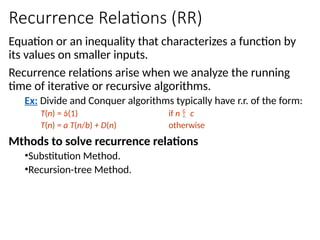
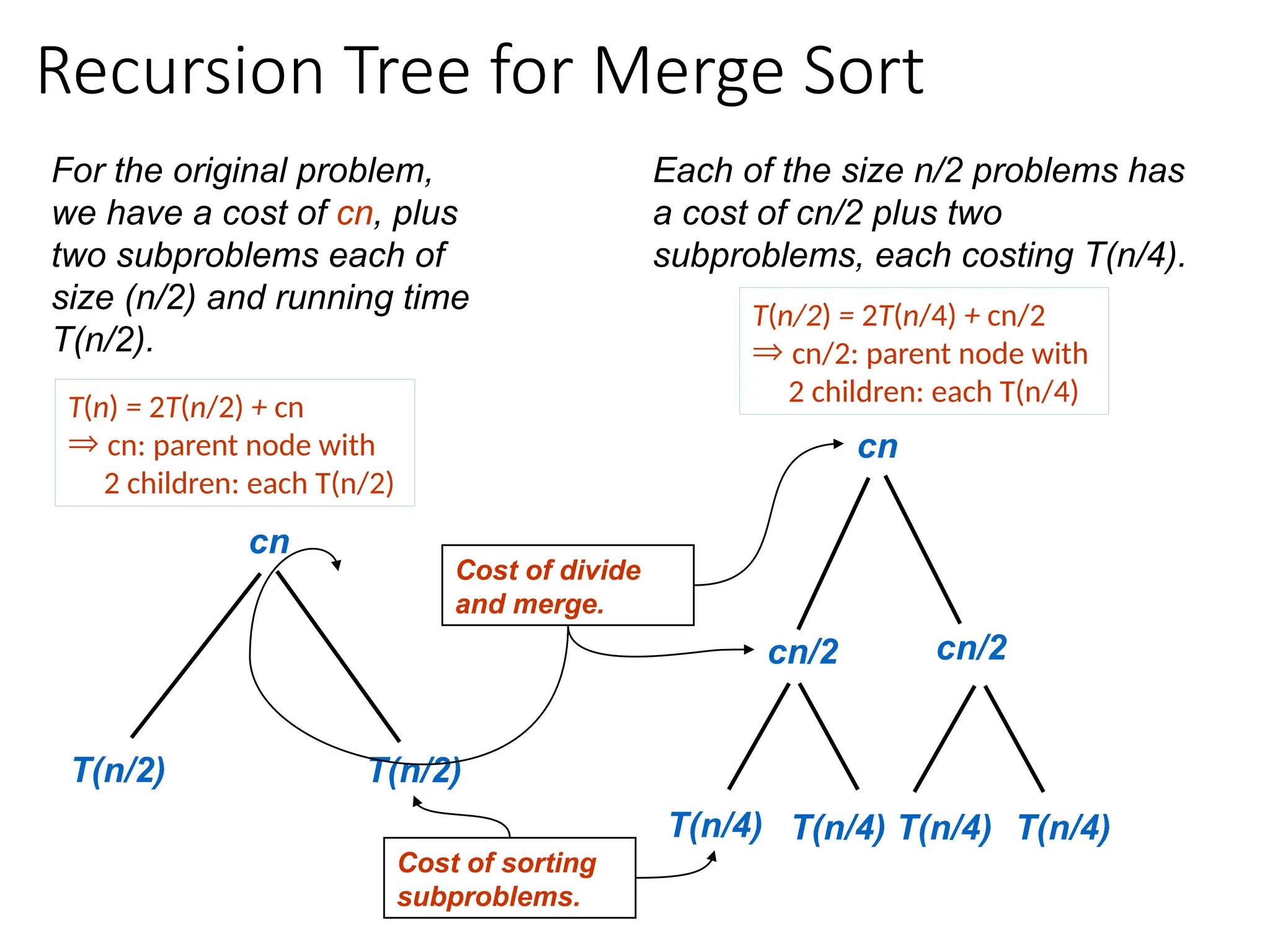
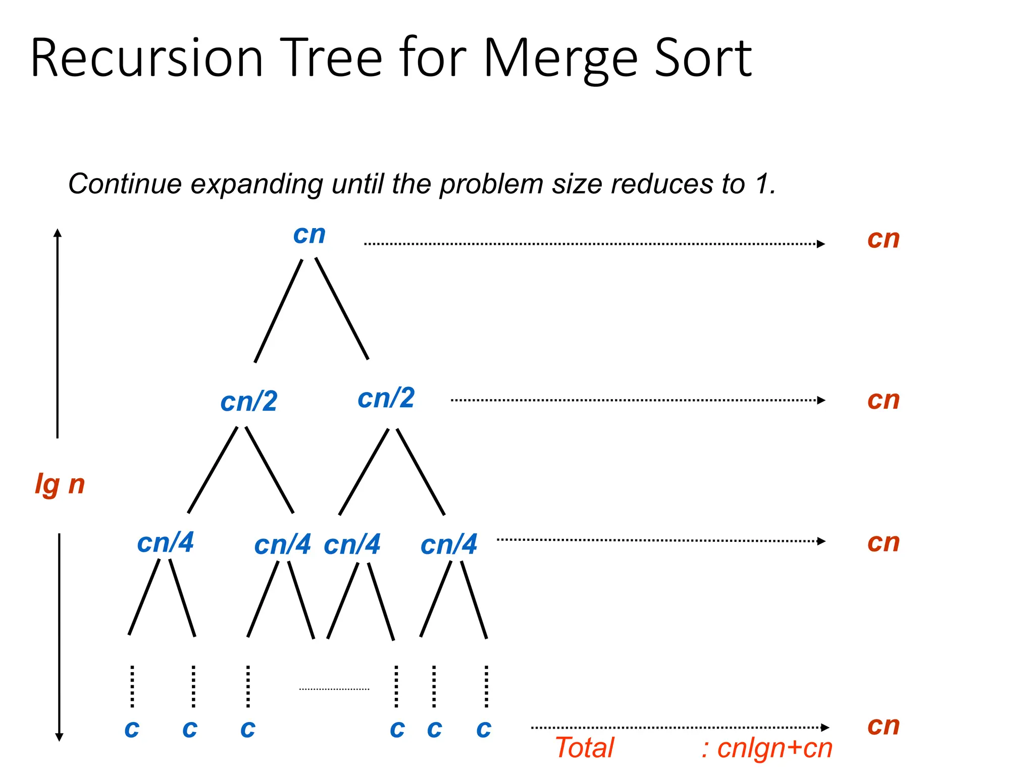
![Substitution Method
Illustration of guessing solution of a r.r. (representing time
complexity of MergeSort) via substitution method:
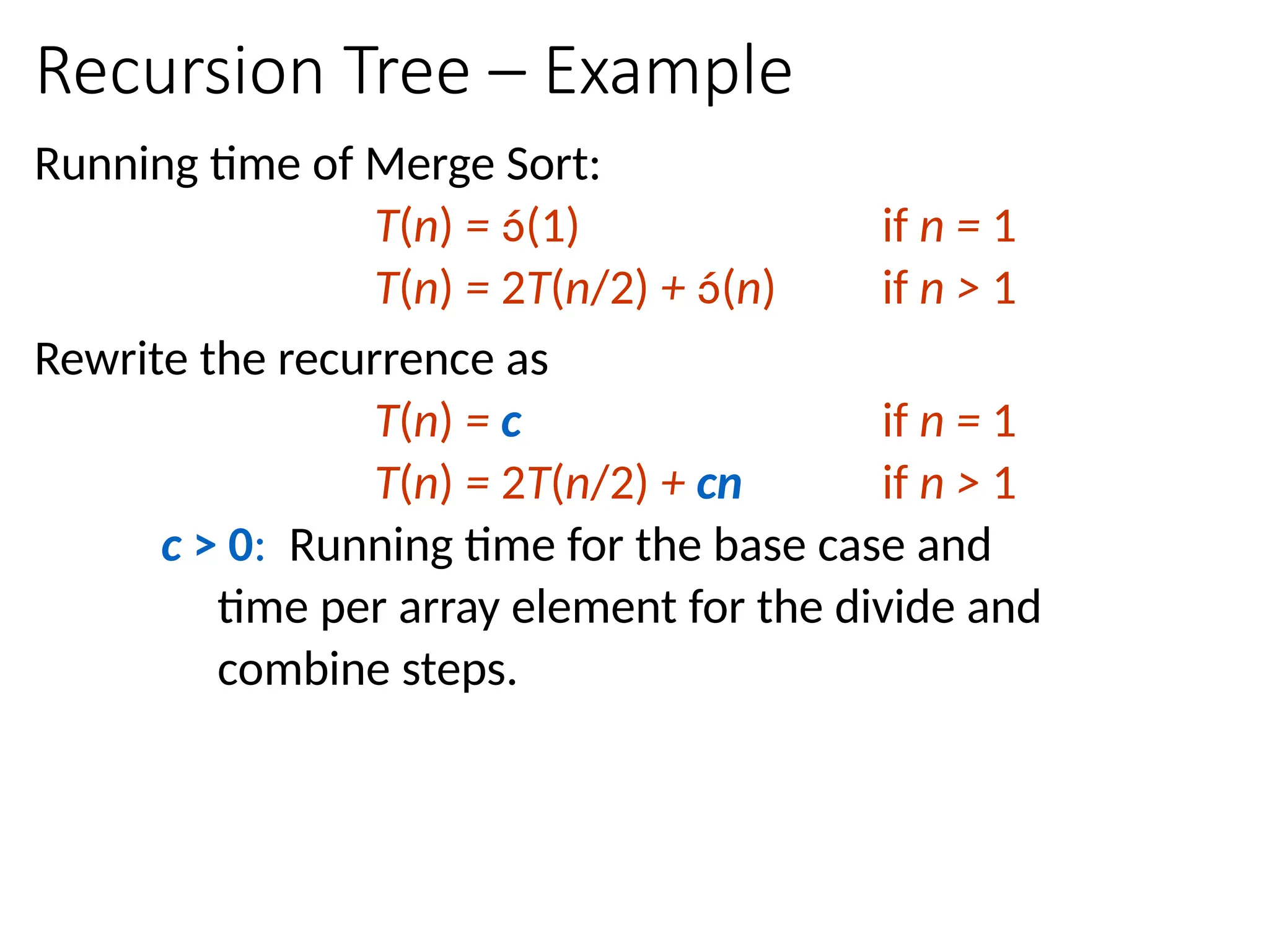
T(n) = 2T(n/2) + cn
= 2(2T(n/4)+cn/2) + cn = 22
T(n/22
) + 2cn
= 22
(2T(n/8)+cn/4) + 2cn = 23
T(n/23
) + 3cn
…
= 2k
T(n/2k
) + kcn [guess the pattern from previous equations]
Let 2k
= n (so that we get T(n/2k
) = T(1) which is known to us)
⸫ T(n) = n T(n/n) + (lg n) cn
= n T(1) + (lg n) cn
= n T(1) + cn lg n
= cn + (lg n) cn which is (n lg n)](https://image.slidesharecdn.com/l2divideconquer-241117011201-6376395f/85/L2_DatabAlgorithm-Basics-with-Design-Analysis-pptx-84-320.jpg)


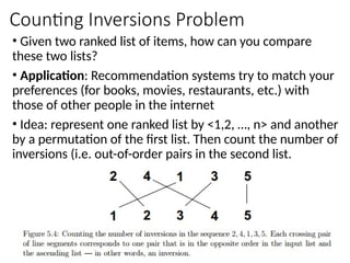
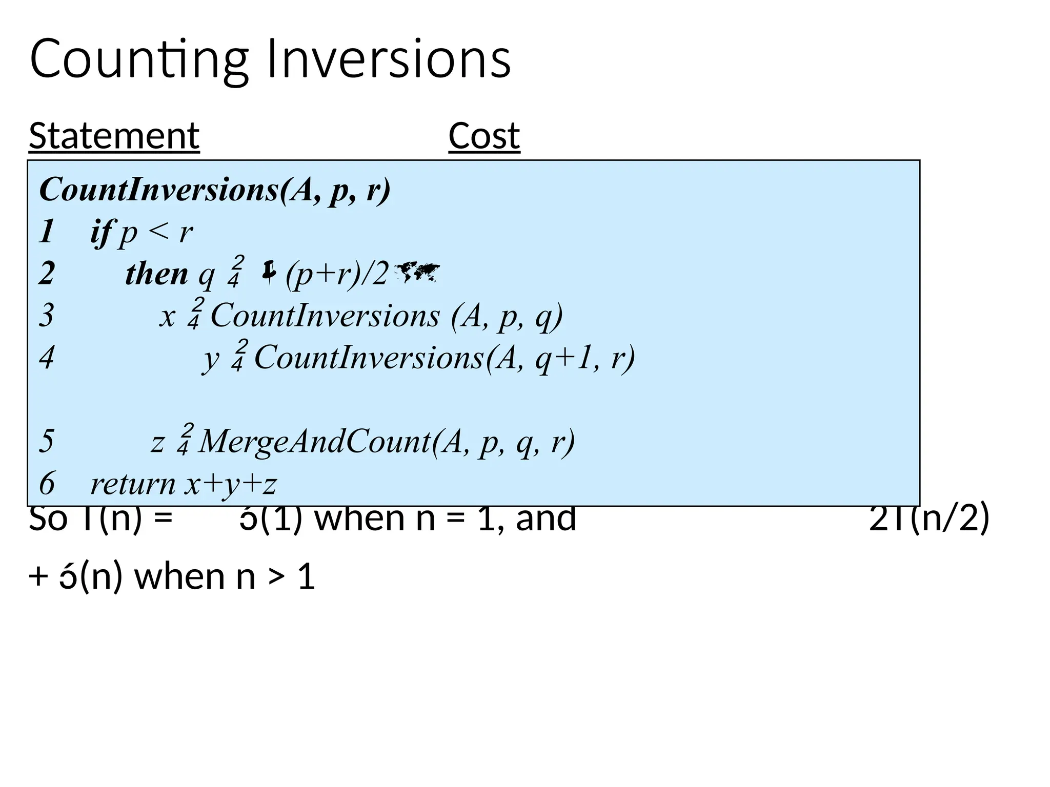
![Merging & Counting Inversions
MergeAndCount(A, p, q, r)
1 n1 q – p + 1
2 n2 r – q
3 for i 1 to n1
4 do L[i] A[p + i – 1]
5 for j 1 to n2
6 do R[j] A[q + j]
7 L[n1+1]
8 R[n2+1]
9 i 1
10 j 1
11 cnt 0
12 for k p to r
13 do if L[i] R[j]
14 then A[k] L[i]
15 i i + 1
16 else A[k] R[j]
17 j j + 1
18 cnt cnt + n1-i+1
19 return cnt
Input: Array containing
sorted subarrays A[p..q] and
A[q+1..r].
Output: Merged sorted
subarray in A[p..r].](https://image.slidesharecdn.com/l2divideconquer-241117011201-6376395f/85/L2_DatabAlgorithm-Basics-with-Design-Analysis-pptx-90-320.jpg)
![A motivating Example of D&C Algorithm
Binary Search (recursive)
// Returns location of x in the sorted array A[first..last] if x is in A, otherwise returns -1
Algorithm BinarySearch(A, first, last, x)
if last ≥ first then
mid = first + (last - first)/2
// If the element is present at the middle itself
if A[mid] = x then
return mid
// If element is smaller than mid, then it can only be present in left sub-array
else if A[mid] > x then
return BinarySearch(A, first, mid-1, x)
// Otherwise the element can only be present in the right sub-array
else
return BinarySearch(A, mid+1, last, x);
Initial call: BinarySearch(A,1,n,key) where key is an user input which is to be sought in A](https://image.slidesharecdn.com/l2divideconquer-241117011201-6376395f/75/L2_DatabAlgorithm-Basics-with-Design-Analysis-pptx-2-2048.jpg)


![Binary Search (recursive) Algorithm
// Returns location of x in the sorted array A[first..last] if x is in A, otherwise returns -1
Algorithm BinarySearch(A, p, q, x)
if last ≥ first then
mid (p+q)/2
// If the element is present at the middle itself
if A[mid] = x then
return mid
// If element is smaller than mid, then it can only be present in left sub-array
if A[mid] > x then
return BinarySearch(A, p, mid-1, x)
// Otherwise the element can only be present in the right sub-array
else
return BinarySearch(A, mid+1, q, x)
return -1 // We reach here when element is not present in A
Initial call: BinarySearch(A,1,n,key) where key is an user input which is to be sought in A
Time: Θ(lg n), why?](https://image.slidesharecdn.com/l2divideconquer-241117011201-6376395f/75/L2_DatabAlgorithm-Basics-with-Design-Analysis-pptx-15-2048.jpg)

![D&C Algorithm Example: Binary Search
Searching Problem: Search for item in a sorted sequence A of n elements
Divide: Divide the n-element input array into two subarray of ≈ n/2 elements
each:
m (p+q)/2
Conquer: Search either of the subarrays recursively by calling BinarySearch on
the appropriate subarray:
if A[m] > x then
return BinarySearch(A, p, m-1, x)
else
return BinarySearch(A, m+1, q, x)
Combine: Nothing to be done](https://image.slidesharecdn.com/l2divideconquer-241117011201-6376395f/75/L2_DatabAlgorithm-Basics-with-Design-Analysis-pptx-17-2048.jpg)
![D&C Example: Merge Sort (Section 2.3)
Sorting Problem: Sort a sequence A of n elements into non-decreasing order:
MergeSort (A[p..r]) //sort A[p..r]
Divide: Divide the n-element input array into two subarray of ≈ n/2 elements
each [easy]:
q (p+r)/2
Conquer: Sort the two subsequences recursively by calling merge sort on
each subsequence [easy]:
MergeSort (A[p .. q]) // A[p .. q] becomes sorted after this call
MergeSort (A[q+1 .. r]) //A[q+1..r] becomes sorted after this call
Combine: Merge the two sorted subsequences to produce the sorted
sequence [how?]](https://image.slidesharecdn.com/l2divideconquer-241117011201-6376395f/75/L2_DatabAlgorithm-Basics-with-Design-Analysis-pptx-18-2048.jpg)


![Merging two sorted subsequeces
Merge(A, p, q, r)
1 n1 q – p + 1
2 n2 r – q
3 for i 1 to n1
4 do L[i] A[p + i – 1]
5 for j 1 to n2
6 do R[j] A[q + j]
7 L[n1+1]
8 R[n2+1]
9 i 1
10 j 1
11 for k p to r
12 do if L[i] R[j]
13 then A[k] L[i]
14 i i + 1
15 else A[k] R[j]
16 j j + 1
Sentinels, to avoid having to
check if either subarray is
fully copied at each step.
Input: Array containing
sorted subarrays A[p..q] and
A[q+1..r].
Output: Merged sorted
subarray in A[p..r].](https://image.slidesharecdn.com/l2divideconquer-241117011201-6376395f/75/L2_DatabAlgorithm-Basics-with-Design-Analysis-pptx-38-2048.jpg)
![Time complexity of Merge
Merge(A, p, q, r) //Let r-p+1 = n
1 n1 q – p + 1 //Θ(1)
2 n2 r – q //Θ(1)
3 for i 1 to n1 //Θ(q-p+1)
4 do L[i] A[p + i – 1]
5 for j 1 to n2 //Θ(r-q)
6 do R[j] A[q + j]
7 L[n1+1]
8 R[n2+1]
9 i 1
10 j 1
11 for k p to r //Θ(r-p+1) = Θ(n)
12 do if L[i] R[j]
13 then A[k] L[i]
14 i i + 1
15 else A[k] R[j]
16 j j + 1
//Total time: Θ(n)
Input: Array containing
sorted subarrays A[p..q] and
A[q+1..r].
Output: Merged sorted
subarray in A[p..r].](https://image.slidesharecdn.com/l2divideconquer-241117011201-6376395f/75/L2_DatabAlgorithm-Basics-with-Design-Analysis-pptx-39-2048.jpg)
![Merge Sort (recursive/D&C version)
MergeSort (A, p, r) // sort A[p..r] via merge sort
1 if p < r
2 then q (p+r)/2 //divide
3 MergeSort (A, p, q) //conquer
4 MergeSort (A, q+1, r) //conquer
5 Merge (A, p, q, r) //combine: merge A[p..q] with A[q+1..r]
Initial Call: MergeSort(A, 1, n)](https://image.slidesharecdn.com/l2divideconquer-241117011201-6376395f/75/L2_DatabAlgorithm-Basics-with-Design-Analysis-pptx-40-2048.jpg)


![Analysis of Merge Sort
Statement Cost
MergeSort (A, p, r) //initial call: MergeSort(A,1,n) T(n) [let]
1 if p < r
2 then q (p+r)/2
3 MergeSort (A, p, q)
4 MergeSort (A, q+1, r)
5 Merge (A, p, q, r)](https://image.slidesharecdn.com/l2divideconquer-241117011201-6376395f/75/L2_DatabAlgorithm-Basics-with-Design-Analysis-pptx-81-2048.jpg)

![Substitution Method
Illustration of guessing solution of a r.r. (representing time
complexity of MergeSort) via substitution method:
T(n) = 2T(n/2) + cn
= 2(2T(n/4)+cn/2) + cn = 22
T(n/22
) + 2cn
= 22
(2T(n/8)+cn/4) + 2cn = 23
T(n/23
) + 3cn
…
= 2k
T(n/2k
) + kcn [guess the pattern from previous equations]
Let 2k
= n (so that we get T(n/2k
) = T(1) which is known to us)
⸫ T(n) = n T(n/n) + (lg n) cn
= n T(1) + (lg n) cn
= n T(1) + cn lg n
= cn + (lg n) cn which is (n lg n)](https://image.slidesharecdn.com/l2divideconquer-241117011201-6376395f/75/L2_DatabAlgorithm-Basics-with-Design-Analysis-pptx-84-2048.jpg)
![Merging & Counting Inversions
MergeAndCount(A, p, q, r)
1 n1 q – p + 1
2 n2 r – q
3 for i 1 to n1
4 do L[i] A[p + i – 1]
5 for j 1 to n2
6 do R[j] A[q + j]
7 L[n1+1]
8 R[n2+1]
9 i 1
10 j 1
11 cnt 0
12 for k p to r
13 do if L[i] R[j]
14 then A[k] L[i]
15 i i + 1
16 else A[k] R[j]
17 j j + 1
18 cnt cnt + n1-i+1
19 return cnt
Input: Array containing
sorted subarrays A[p..q] and
A[q+1..r].
Output: Merged sorted
subarray in A[p..r].](https://image.slidesharecdn.com/l2divideconquer-241117011201-6376395f/75/L2_DatabAlgorithm-Basics-with-Design-Analysis-pptx-90-2048.jpg)


![Agentic Systems and Compliance - A brief intro [1.2]](https://cdn.slidesharecdn.com/ss_thumbnails/agenticsystemsandcompliace-1-251018025303-958a42ec-thumbnail.jpg?width=600ounds&width=560&fit=bounds)

![Matrix and determinant URT [Autosaved].pptx](https://cdn.slidesharecdn.com/ss_thumbnails/matrixanddeterminanturtautosaved-251018190340-9e6a6deb-thumbnail.jpg?width=600ounds&width=560&fit=bounds)


![RTP_AR_Basic_Learners' Workbook_KS2 [FOR REPRODUCTION] (1).pdf](https://cdn.slidesharecdn.com/ss_thumbnails/rtparbasiclearnersworkbookks2forreproduction1-251016024943-e51a16ac-thumbnail.jpg?width=600ounds&width=560&fit=bounds)